Stochastic applications of media theory: random walks on weak orders or partial orders

(1)

www.elsevier.com/locate/dam

Stochastic applications of media theory: Random walks on weak

orders or partial orders

Jean-Claude Falmagne

a,_∗

_{, Yung-Fong Hsu}

b

_{, Fabio Leite}

c

_{, Michel Regenwetter}

d a_{Department of Cognitive Sciences, University of California, Irvine, CA 92697, USA}

b_{Department of Psychology, National Taiwan University, Taiwan} c_{Department of Psychology, Ohio State University, USA}

d_{Psychology and Political Science, University of Illinois, Urbana-Champaign, USA}

Received 7 May 2004; received in revised form 15 December 2004; accepted 11 April 2007 Available online 15 August 2007

Abstract

This paper presents the axioms of a real time random walk on the set of states of a medium and some of their consequences, such as the asymptotic probabilities of the states. The states of the random walk coincide with those of the medium, and the transitions of the random walk are governed by a probability distribution on the set of token-events, together with a Poisson process regulating the arrivals of such events. We examine two special cases. The first is the medium on strict weak orders on a set of three elements, the second the medium of strict partial orders on the same set. Thus, in each of these cases, a state of the medium is a binary relation. We also consider tune in-and-out extensions of these two special cases. We review applications of these models to opinion poll data pertaining to the 1992 United States presidential election. Each strict weak order or strict partial order is interpreted as being the implicit or explicit opinion of some individual regarding the three major candidates in that election, namely, Bush, Clinton and Perot. In particular, the strict partial order applications illustrate our notion of a response function that provides the link between theory and data in situations where, in contrast to previous papers, the permissible responses do not span the entire set of permissible states of the medium.

Keywords:Media theory; Partial orders; Random walk; Stochastic process; Weak orders

A medium is a particular semigroup of transformations, called ‘tokens,’ on a finite set of states (cf.[4,6]). The axioms defining a medium, which are recalled by[17]in this volume (see also[3]), make such a semigroup especially suitable for a stochastic application in the shape of a random walk on its set of states. (Thus, the states of the random walk coincide with those of the medium.) The basic idea is that there is a positive probability distribution !: T →]0, 1] : " #→ !"

on the set T of all tokens, such that the probability of a transition from state S to some other state T is equal to !" if S"= T , and vanishes otherwise. A realization of the random walk is obtained by sequentially sampling this

distribution. Under these hypotheses, the symmetry inherent in a medium ensures that the asymptotic probabilities of the random walk exist and are easy to describe; namely: the asymptotic probability of some state S is proportional to the product of the probabilities !"of all the tokens " whose application results in a state closer to S. (In medium

∗Corresponding author. Tel.: +1 949 824 4880; fax: +1 949 824 1670. E-mail address:[email protected](J.-C. Falmagne).

(2)

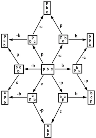
Fig. 1. Graph of the medium of the 13 (strict) weak orders on a set of three elements_{{b, c, p}. The edges represent the positive and the negative} tokens, which transform a state into one closer to a linear order. Edges bearing the same label represent the same token. Reversing an edge would yield the reverse token. The reader will notice that our labeling of the edges slightly simplifies the notation of the tokens.

terminology, the asymptotic probability of S is the normalized product of all the !"’s such that " belongs to the ‘content’ of S.)

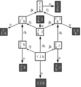
Such a mechanism may provide a model for the evolution of a biological, social or physical system subjected to a constant probabilistic barrage of ‘token-events,’ each of which may induce a ‘mutation’ of its state taking the form of an addition or a removal of some constituent feature. The applications described in this paper belong to the social sciences. In one application, the states of the medium are the 13 possible (strict) weak orders (rankings with possible ties) on a set of three elements. A token consists in moving (or removing) an element to (from) the top or bottom of the ranking. The graph of this medium is given inFig. 1, adapted from[4]or[20]. An examination of this figure in the context of the axioms of a medium (which are recalled in[17]) should easily convince the reader that the graph is that of a medium. In the second application, the medium in question is defined by the set of 19 (strict) partial orders on a set of three elements, with a token consisting either in the addition of a pair to a partial order, or in the removal of a pair from it, in either case creating another partial order. This defines a medium because the family of all partial orders on a finite set is well graded in the sense of[2]. In this connection, see also[4,6,18], as well as similar results obtained previously by[1](see, furthermore,[15]). We provide the graph of the partial order medium inFig. 2.

In the graphs ofFigs. 1 and 2, the labeled oriented edges represent all those tokens whose application results in a state closer to one of the six linear orders. The ‘reverse’ tokens are obtained by reversing the edges. (The reverse of a token " is the token˜" such that, for any two distinct states S and T, we have S" = T if and only if T ˜" = S; cf. Definition 1.) Note the typical ‘parallelism’ of all the edges representing the action of any given token on the states. In our empirical illustration, each of the weak orders or partial orders corresponds to the implicit or explicit opinion of some individual regarding the three major candidates at the 1992 United States presidential election, that is, Bush, Clinton and Perot. Appropriately, the base set of options is denoted by{b, c, p}.

(3)

Fig. 2. Graph of the medium of the 19 (strict) partial orders on a set of three elements_{{b, c, p}. The edges represent the tokens transforming a state} into one closer to a linear order. Edges bearing the same label represent the same token. Reversing an edge (and transposing the letters of its label) would yield the reverse token. As inFig. 1, our labeling of the edges slightly simplifies the notation of the tokens. For example, we write here bc rather than"bc. Ignore the shadowing for the moment.

In the first section of this paper, we begin by stating the axioms of a general random walk on the states of a medium along the lines of the first paragraph above. These axioms formalize a situation in which the arrival times of the token-events are governed by a Poisson process. This results in a model capable of describing the real time, feature-by-feature stochastic evolution of a system whose successive transformations are consistent with the axioms of a medium. Next, we derive the main asymptotic results, with special attention to those predictions of interest in the application.

In the second section, we present applications of this model to weak order and partial order models of voter preferences and briefly illustrate these applications on data from the National Election Study panel[14]pertaining to the 1992 presidential election in the United States. Such data provide reliable information about evaluations of the three major candidates in that election for a substantial sample of the American electorate at two time points (one shortly before and one shortly after the election).

1. A real time random walk on the states of a medium

Our developments in this section substantially generalize those in[5]. 1.1. Notation

Definition 1. We denote a basic medium by the ordered pair (S, T). Thus, S is the set of its states, and T the set

of its tokens. A token "∈ T is a transformation S #→ S" of some state S into some possibly different state S". For the axioms defining a medium, as well as basic terminology (such as the concepts of an ‘effective’ message or token,

(4)

a ‘straight’ message, the ‘content’ of a state), see[4,6]or[17]in this volume. We recall that ˜" denotes the reverse of token ", that is, for any states S%= T , we have S" = T iff T ˜" = S; thus, ˜˜" = ".

We assume that there exists some initial probability distribution

#: S → [0, 1] : S #→ #S

on the set of states, and a positive probability distribution !: T →]0, 1] : " #→ !"

on the set of tokens. The evolution is described in terms of three collections of random variables. For t ∈]0, ∞[,

St denotes the state of the random walk at time t,

Nt specifies the number of tokens that have occurred in the half-open interval of time]0, t] and

Tt is the last token to occur before or at time t. We set Tt= 0 if no token has occurred, that is, if Nt= 0. Thus, St takes its values in the set S of states, Nt is a nonnegative integer and Tt ∈ T ∪ {0}. The random variables

Nt will turn out to be the counting random variables of a Poisson process governing the delivery of the token-events. The following random variables will also be convenient:

Nt,t+$= Nt+$− Nt

denoting the number of tokens in the half-open interval]t, t + $].

1.2. Axioms

The three axioms below specify the stochastic process (Nt,Tt,St)t >0up to the parameters (#S)S_∈S and (!")"∈T for the two probability distributions, and a parameter % > 0 specifying the intensity of the Poisson process.

[I] (Initial state). Initially, the system is in state S with probability #S. The system remains in that state at least until the occurrence of the first token-event. That is, for any S ∈ S and t > 0

P(St= S|Nt = 0) = #S.

The two remaining axioms specify the process recursively. The notation Et stands for any arbitrarily chosen history of the process until and including time t > 0; E0denotes the empty history.

[T] (Occurrence of the tokens). The occurrence of the token-events is governed by a homogeneous Poisson process of intensity %. When a Poisson event is realized, the token " is selected with probability !">0, regardless of past events. Thus, for any nonnegative integer k, any real numbers t > 0 and $ > 0, and any history Et,

P(Nt,t_+$= k|Et)=

(%$)k_e_−%$

k! , (1)

P(Tt_+$= "|Nt,t_+$= 1, Et)= P(Tt_+$= "|Nt,t_+$= 1) = !">0. (2) [L] (Learning). If R is the state of the system at time t, and a single token " occurs between times t and t+ $, then the state at time t+ $ will be R" regardless of past events before time t. Formally,

P(St+$= S|Tt+$= ", Nt,t+$= 1, St= R, Et)= P(St+$= S|Tt+$= ", Nt,t+$= 1, St= R) =! 1 if S = R",

0 otherwise.

Remarks 2. (a) Axioms [I] and [L] formalize the random walk mechanism. We can generalize Axiom [L] by assuming

that the transition probabilities depend not only on the tokens, but also on the states of the system. We do not explore this possibility here (however, see Remark 6). (b) Axiom [T] can also be generalized. Many of the results still hold if we assume that we have a general renewal process, rather than a Poisson process. This is true in particular for the asymptotic result in Theorem 4.

(5)

1.3. Basic results Notice that P(St_+$= S|St= R) = ∞ " k₌₀ P(St_+$= S|Nt,t_+$= k, St = R)P(Nt,t_+$= k|St = R) = ∞ " k₌₀ P(St+$= S|Nt,t+$= k, St = R)P(Nt,t+$= k) (3)

by the Poisson process Axiom [T]. For any pair (R, S) of distinct states, there is at most one token " such that R"= S (cf.[6, Theorem 6(ii)]). Such a token is said to be effective for R. For any state R, we denote by TRthe subset of all

tokens that are effective for R and we write TR= T\TR. We have successively, using Axioms [T] and [L],

P(St+$= S|Nt,t+$= 1, St= R) =" "∈T P(St_+$= S|Tt_+$= ", Nt,t_+$= 1, St= R)P(Tt_+$= "|Nt,t_+$= 1, St= R) =" "∈T P(St_+$= S|Tt_+$= ", Nt,t_+$= 1, St= R)P(Tt_+$= "|Nt,t_+$= 1) =      !" if R%= S = R", ' "∈TR!" if R= S = R", 0 in all other cases,

which does not depend on t or $. Indeed, the first factor in each term of the sum in the first and second equation is equal to 0 or 1. The value is 1 in exactly two cases: R%= S = R" (case 1 in the right-hand side of the last equation) or R= S = R" (case 2). The following definition is thus justified:

&R,S= P(St+$= S|Nt,t+$= 1, St = R). (4)

As the right-hand side of (4) does not depend upon either t or $, this implies that, regardless of the times of occurrence of the tokens, the sequence of states, which we denote by (Mn)_n_∈N, is a homogeneous Markov chain with 1-step transition probabilities &R,S, (R, S∈ S). We refer to (Mn)as the companion Markov chain of the process (St). Accordingly, we can define

&R,S(k)= P(St_+$= S|Nt,t_+$= k, St= R) = P(Mn_+k= S|Mn= R) (5) to denote the k-step transition probabilities of the Markov chain (Mn)_n_∈N. Note that &R,S= &R,S(1). Using (3), (5) and (1) of Axiom [T], we obtain:

Theorem 3. The stochastic process (St)is a homogeneous Markov process, with transition probability function pR,S($)= P(St_+$= S|St= R) = ∞ " k₌₀ &R,S(k)(%$) k_e_−%$ k! .

Thus, pR,S($) is the probability of a transition from state R to state S in $ units of time. We recall that two distinct states R and S of a medium are called adjacent if there exists some token " such that R"= S or, equivalently, S˜" = R. Because the only possible transitions are those occurring between adjacent states, we also refer to the Markov process (St)as a random walk process.

We now turn to the asymptotic probabilities of the states. Using the companion Markov chain, the asymptotic probabilities of the states of the process (St)are easily computed. They are given in Theorem 4. We recall that (S

(6)

denotes the content of the state S in the medium (S, T), that is, (Sis the set of all tokens belonging to the content of some straight message producing S.

Theorem 4. The companion homogeneous Markov chain (Mn)is irreducible and aperiodic. Accordingly the

asymp-totic probabilities of the states exist and coincide with those of the homogeneous Markov process (St). We have, in fact,

for any S_{∈ S,} lim n→∞P(Mn= S) = limt→∞P(St= S) = ) "∈(S!" ' R∈S ) '∈(R!' . (6)

This means that, if the process has been running for a long time, we may be able to explain the empirical preference distribution with a parsimonious asymptotic distribution.

The proof uses the following well-known fact:

Lemma 5. Let (mR,S)R,S∈Sbe the transition matrix of a regular Markov chain on a finite set S, and let (: R #→ (R

be a probability distribution on S. Suppose that, for all R, S∈ S, we have (R· mR,S = (S· mS,R.

Then ( is the unique stationary distribution of the Markov chain.

It suffices to verify that (R='S∈S(S· mS,R for all R∈ S.

Proof of Theorem 4. The Markov chain (Mn)is irreducible because: (i) as a consequence of the axioms of a medium, for any two distinct states R and S, there is a straight message transforming R into S; and (ii) !">0 for any token ". It is also aperiodic. Indeed, to show this, we only have to prove that

&S,S>0, (7)

for at least one state S. Since (S, T) is a medium, it has at least two states. So, let S and R be these two states of the medium. There must exist a straight message producing R from S. Let " be the first token of that message. The reverse token˜" must be ineffective for S. By Axioms [T], [L], we obtain &S,S!!˜">0, establishing Eq. (7). Thus, the Markov chain (Mn)is irreducible and aperiodic. Accordingly, the asymptotic probabilities of the states of that Markov chain form a unique stationary distribution.

It remains to show that the stationary distribution is that given by Eq. (6). We use Lemma 5, and prove that for any R, S∈ S, and writing K for the denominator in (6),

1 K  , "∈(R !"   &R,S= 1 K  , "∈(S !"   &S,R. (8)

Denoting by ) the symmetric difference between sets, we consider three cases: &R,S= &S,R= 0, |R!S| > 2 (Case 1),

&R,S= &S,R= &S,S>0, R= S (Case 2),

&R,S= !'>0, &S,R= !˜'>0, R!S= {', ˜'} (Case 3).

(for some '∈ T in Case 3). In Case 1, both sides of (8) vanish, whereas in Case 2, the two expressions on both sides of the equation are identical. Eq. (8) also holds in Case 3 since it is equivalent to

  , "∈((R∩(S) !"   !'!_˜'=   , "∈((R∩(S) !"   !_˜'!'.

(7)

Remark 6. In some situations, it would make sense to suppose that the conditional probability of a transition from

some state R of the random walk to some state S%= R depends not only on the token " such that R" = S, but also on R. For example, we might have both R"= S and W" = S but the transitions would have different probabilities denoted, for example, by !"*Rand !"*W, the first factor representing the contribution of some external source, and the second one the specific effect on a particular state. A close reading of the above proof indicates that the argument used to justify Eq. (8) would also apply in such a case. A version of Theorem 4 would thus hold, with the products in Eq. (6) having many more factors. This would result in a model with|T| · |S| − 1 independent parameters, which might be of some interest in a case where extensive sequential data are available. Note that submodels may be considered in which the number of parameters *Rmight be substantially smaller than|S|.

Using Theorems 3 and 4, an explicit expression can be obtained for the asymptotic joint probability of observing the states R and S at time t and time t+ $, respectively. We write, as before, &R,S(k)for the k-step transition probability from the state R to the state S in the companion Markov chain on S, and pR,S($) for the probability of a transition between the same two states, in $ units of time, in the stochastic process (St). Defining

qR= lim t_→∞P(St = R), we get lim t→∞P(St= R, St+$= S) = limt→∞(P(St= R)P(St+$= S|St = R)) = qRpR,S($).

Thus, the asymptotic (t → ∞) joint probability for the random walk to occupy state R at time t and state S at time t+ $ is the product of the asymptotic probability of state R, which is known from Theorem 4, by the probability that the random walk moves from state R to state S in $ units of time. The latter was obtained in Theorem 3. Accordingly, we have:

Theorem 7. For all states R and S and all $ > 0,

lim t_→∞P(St = R, St+$= S) = ) "∈(R!" ' V_∈S ) '∈(V!' ∞ " k=0 &R,S(k)(%$) k_e_−%$ k! .

In our application, this equation provides the mathematical formula needed to model and predict preferences in a longitudinal survey where participant responses are recorded at two time points that are separated by some amount of time $.

2. The case of unobservable states: the response function

In certain important situations some or all of the states of the medium fail to be directly observable. This may happen, for example, because of some inherent limitations in the observation instrument. In the context of an opin-ion poll, this is likely to occur because the questopin-ions may be formulated in a fashopin-ion that forces answers in a specific format that need not exactly reflect the respondents’ states of mind. To deal with such cases, we must dissociate the state of the random walk on the medium at time t > 0 from the observations that are made at that time.

We consider here the case in which what is observed at any time t is always a state of the medium, i.e., an element of S, yet such an observation may not be identical to the state of the random walk at time t.

Definition 8. To this effect we introduce a new collection of random variables Rt, t ∈]0, ∞[ denoting the response at time t. The random variables Rt take their values in a distinguished subset ˇS⊂ S of the set S of states, called the response set. Note that the random variables Rt are defined for any t > 0 even though, in practice, they may not be

(8)

recorded. We also define a (probabilistic) response function +: S × ˇS → [0, 1] : (S, R) #→ +(S, R),

" R_{∈ ˇ}S

+(S, R)= 1 (S ∈ S).

In effect, +(S, R) is the conditional probability of overt response R ∈ ˇS given latent preference state S ∈ S. This function may of course introduce additional parameters in the model. The use of this function is regulated by the response axiom below, which assumes that the responses only depend on the states via the function +, and moreover that, given the states, the responses are independent events.

[R] (Responses). For any choice of times t1<· · · < tn, and any R1, . . . , Rnin ˇS and S1, . . . , Snin S, we have

P(Rt1= R1, . . . ,Rtn= Rn|Stn= Sn, . . . ,St1 = S1,Etn)= n , i₌₁

+(Si, Ri).

The following result is immediate:

Theorem 9. For all pairs (R, R,₎_{in ˇ}_S_{× ˇS and any $ > 0, we have} lim t_→∞P(Rt = R, Rt+$= R ,₎₌ " (S,S,)_∈S×S +(S, R)+(S,, R,) lim t_→∞P(St= S, St+$= S ,_).

Note that Theorem 7 gives us an explicit formula for the last factor in the above equation. Consequently, in those cases in which the function + is specified (possibly up to some numerical parameters), this theorem yields a prediction for the joint probability of observing, for large values of t, the responses R and R,_{at times t and t}_{+ $. Like Theorem} 7, this theorem provides the necessary mathematical formulae to model and predict preferences in the panel study of our empirical application. In our formulation here, we have added the response mechanism to cover those situations where the state space and the survey response space are not identical.

3. Applications to the analysis of an opinion poll: random walks on weak orders or partial orders

As we have indicated at the onset of the paper, we illustrate the theory in a social science context, with data provided by a presidential election opinion poll. We use two models, the combinatoric core of which are the weak order and the partial order media. In addition, we consider a natural generalization of both of these media to accommodate an important mechanism of persuasion.

We briefly review the definition of some standard concepts.

Definition 10. We abbreviate the ordered pair (j, k) as jk. If R and S are two (binary) relations, we write RS =

{!k|∃j, !Rj, jSk} for their relative product, R−1= {jk|kRj} for the inverse of the relation R. If R is a relation on C, thus R ⊆ C × C, we denote by R = (C × C)\R the complement of R (with respect to C), and by IdCthe identity relation on C. A relation R on C is

transitive if RR⊆ R,

asymmetric if R∩ R−1= ∅,

negatively transitive if RR⊆ R,

complete if R∪ R−1∪ IdC= C × C.

A (strict) partial order is an asymmetric and transitive relation. A (strict) weak order is an asymmetric and negatively transitive relation. A (strict) linear order is a transitive, asymmetric, and complete relation.

(9)

Table 1

Types of tokens in the weak order medium, their psychological interpretation, and the transformation that each token defines on the collectionWO of weak orders on_{{b, c, p}, with !, j and k any distinct elements of {b, c, p}}

Notation Psychological interpretation Transformation

"! !is the ‘best’ option S"!=

       {!j, jk} if S = {!k, jk} {!j, !k} if S = ∅ S otherwise. /

"! !is not the ‘best’ option S/"!=

       {!k, jk} if S = {!j, jk} ∅ if S_{= {!j, !k}} S otherwise

"−k kis the ‘worst’ option S"−k=

       {!j, jk} if S = {!j, !k} {!k, jk} if S = ∅ S otherwise 0

"−k kis not the ‘worst’ option S0"−k=

       {!j, !k} if S = {!j, jk} ∅ if S= {!k, jk} S otherwise For simplicity in the third column, the weak orders are represented by their Hasse diagrams.

In what follows, we occasionally denote a partial order by0 or some similar symbol. In such cases, we sometimes abbreviate the conjunction[¬(j 0 k) and ¬(k 0 j)] by j ∼ k. The same type of convention applies when the partial order is denoted by0,_or₀,,_.

3.1. The medium of weak orders on three alternatives

Strict weak orders have a natural interpretation and long tradition as mathematical representations of preferences (see, e.g.,[9,11,13]). For three choice alternatives (e.g., political candidates) there exist 13 possible weak order pref-erence states. The random walk on the weak order medium has been developed by [7] and successfully applied to a national survey by [20]. Note that [16] has developed a fairly natural medium interpretation of the collec-tion of all weak orders on a set of n elements, for arbitrary n. Evidently, the random walk results given in this paper would be applicable to such cases. So far, however, no empirical study with n > 3 has been performed. In

Table 1 we provide an overview of the types of tokens in the weak order medium, their psychological interpre-tation, as well as the transformation that each token defines on the collection WO of weak orders over{b, c, p}. In our application, we assume that the weak orders are directly observable, i.e., there is no need for a response function.

The tokens of the weak order medium of this example can be interpreted psychologically as capturing persuasion mechanisms and how they effectively operate on preference states. Suppose that at time t, a potential voter in the 1992 presidential election prefers Perot to Bush, and Bush to Clinton; so, in the random variable notation of Definition 1, this voter is in state St= 0 with p 0 b 0 c. Imagine that this voter, at some time t,> t, is exposed to some

information convincing him or her that Perot is not the best candidate. Consulting the graph ofFig. 1orTable 1, we see that, in such a case, the voter moves Perot down in the ranking. The state of the voter at time t,_{is thus S}_t_,_{= 0},

with b0,c, p0,c. Note that the voter may not be tested at time t,, so that the state St, = 0,may remain latent, until

either the voter is tested at some time t,,> t,and responds then according to state St,,= 0,, or some new information

comes around which changes state0, into some other state according to the possible transitions described by the graph ofFig. 1orTable 1. We do not discuss this model in more details here, but refer the interested reader instead to

(10)

Table 2

Types of tokens in the partial order medium, their psychological interpretation, and the transformation that each token defines on the collectionPO of all partial orders on_{{b, c, p}, with !, j and k any distinct elements of {b, c, p}}

Notation Psychological interpretation Transformation "j k jis ‘preferable’ to k S"j k= 1_S ∪ {jk} if S ∪ {jk} ∈PO S otherwise 2 "j k jis not ‘preferable’ to k S"2j k= 1 S\{jk} if S\{jk} ∈PO S otherwise

3.2. The medium of partial orders on three alternatives

Like weak orders, partial orders and their special case, semiorders, have a long tradition in the decision sciences as formal representations of preference[12,8,19]. A random walk model based on semiorders is feasible along lines slightly different from those of the weak order example just described. The interest of the semiorder model is that it makes less constraining assumptions concerning the latent mental states of the voters, at those times when they are not forced to express their choices according to the instructions by the poll takers. In the empirical study described here, the choice set contains only three alternatives. In such a case, any partial order is automatically a semiorder. Accordingly, only partial orders are mentioned in the sequel. We denote by PO the set of all 19 partial orders on{b, c, p}, of which 13 are the weak orders already discussed above. In our application of this model, we have S= PO and ˇS = WO.

The tokens of the partial order medium differ substantially from those of the weak order medium. However, they can, in turn, again be interpreted psychologically as capturing persuasion mechanisms and how they effectively operate on preference states. Here, each token provides information about the relative standing of only a pair of candidates in the partial order. As made clear byFig. 2orTable 2, the effect of a token, if any, consists either in the addition of a pair to, or in the removal of such a pair from, the current partial order state, thereby creating a different partial order state.

3.3. Tune in-and-out extensions: the frozen states

While providing a good statistical fit to the data, the empirical application of the weak order random walk by[20]

suffered from the statistical shortfall of underestimating the number of respondents in a survey who provide the same ranking of the candidates at two different time points. This shortfall was discovered and redressed by[10]. The basic idea of their modification is to introduce additional states to the medium, called ‘frozen states.’ Each of these states is linked only to its ‘active sibling’ (one of the ‘old’ states), and corresponds to the same weak order, or partial order, depending on the model. For concreteness, we consider the case in which the original model is the random walk on the medium of partial orders on three alternatives. We suppose that each partial order arises, as a state, both in an active form and in a frozen form. (We are thus doubling the number of states.) A new set of tokens is defined according to the following rule: the tokens in the original set T are redefined so that they are effective only on the active states, whereas they have no effect on the frozen states. In addition, for each active state S, there is a new token oScalled tune

outtoken, which transforms that state into its frozen sibling S∗_{, but has no effect on any other state. Thus, S}∗_{is the}

frozen sibling of S and S is the active sibling of S∗_{. The reverse of o}_S_{is the tune in token i}_S_{transforming S}∗_{into S but}

being ineffective for any other state. To sum up, and generalizing[10]from the weak order medium to general media, denoting by T∗the set of all tune in and tune out tokens, and writing (T= T ∪ T∗, we have thus, for any states S and T, with S active and T arbitrary,

TiS= !

S if T = S∗

T otherwise and oS= 2iS.

The generic graph ofFig. 3, which describes the extended partial order medium for three alternatives, illustrates this development and makes clear that the resulting semigroup is indeed a medium, and so all the random walk results presented in the first part of this paper apply. In the context of a political campaign, where we use states to represent

(11)

Fig. 3. Generic graph of the partial order tune in-and-out medium. Unshaded states are the active partial orders of the original medium, shaded states are their frozen siblings. Reversing an edge would yield the reverse token. As in previous figures, our labeling of the edges slightly simplifies the notation of the tokens. In particular, we denote the tune out tokens oSsimply by o.

preferences and tokens to represent persuasion processes and their effect on the preference states, tune out tokens correspond to events that make a given voter lose interest in the campaign. By this we mean events that render that voter impervious to all matters related to their preferences regarding the candidates, unless and until a special event occurs which triggers the application of a tune in token specific to the voter’s state. Such a tune in token makes the voter pay attention to the campaign again.

Below, we briefly discuss applications of the tune in-and-out extensions to the 1992 national opinion poll, with highly improved results over the predecessor models. Note that the concept of frozen states may be of interest in a very different context; namely, that of a random walk on a medium describing the evolution of biological or artificial organisms. Such frozen states may then be used to represent those cases in which the evolution of some organism is temporarily or permanently blocked.

3.4. Empirical illustration on 1992 National Election Study data

A standard technique in opinion polls consists in asking the respondents to numerically rate the alternatives using the so-called ‘feeling thermometers.’ Such a technique was used in the data set we analyze, namely the 1992 National Election Study by the Interuniversity Consortium for Political and Social Research at the University of Michigan[14]. In this national survey, 2032 respondents rated, e.g., the three major candidates, Bush, Clinton and Perot, on an integer valued scale from 0 to 100, before and after the election, at two time points that were separated by a few months. A rating of zero expressed ‘cold feelings,’ a rating of 50 expressed ‘neutral feelings,’ and a rating of 100 expressed ‘warm feelings’ towards a given candidate.

Like[20]our data analysis only retains the order of the ratings for the candidates provided by the respondents. The first step is thus a recoding of each original rating set [(Bush, x), (Clinton, y), (Perot, z)] with x, y, z∈ {0, 1, . . . , 100} into a weak order. For example, whatever the values of x, y, z, the outcome z > y > x is coded as the linear order p0 c 0 b, while x = z > y is coded as the weak order b∼,p0,c.

In the case of the weak order model, the states of the medium are observable and such a recoding suffices in order to obtain the pair of states occupied by all the respondents at the times they were polled. If we assume that the process is at asymptote at the time of the first poll, Theorem 7 is immediately applicable, with $ measuring the interval between the two polls. Specifically, the observed joint frequencies of all the weak order pairs (0, 0,)can be predicted from the limit joint probabilities limt_→∞P(St= 0, St_+$= 0,). In turn, these can be computed (with0 =R and 0,= S) from

the right-hand side of the equation in Theorem 7, in which the values of the token probabilities !"and of the intensity %

(12)

model were reported in[20]and were satisfactory, with the reservation, mentioned earlier and discovered by[10], that the probabilities of the pairs (0, 0) of identical states on both polls tended to be underestimated.

The situation is slightly more complicated when we apply the partial order model or one of the tune in-and-out models to empirical data because some states are unobservable. In the partial order medium, for instance, the states {!j} (! is preferred to j and both are indifferent to k) are unobservable, for every choice of distinct !, j ∈ {b, c, p}. For the tune in-and-out models all states may be unobservable in the sense that each active state and its frozen sibling may lead to identical or indistinguishable responses. Thus, in order to apply the partial order model or the tune in-and-out extensions of either model to empirical data, we must specify a response function + of Definition 8, Axiom [R] and Theorem 9.

We begin with the partial order model, in which the states{!j} never occur as observable responses. Here, S = PO, ˇS = WO. In general, we assume 12 additional parameters, ,!j,!kand ,!j,kj (with distinct !, j, k), in the model (two

for each of the shaded vertices in the graph ofFig. 2), with the constraints 0#,!j,!k,0#,!j,kj, and ,!j,!k+ ,!j,kj#1.

We define the response function + so that each state{!j} is transformed into one of its three neighboring states (in the graph ofFig. 2) as follows. For{!j} ∈ PO with distinct !, j ∈ {b, c, p}, and S ∈ WO,

+({!j}, R) =      ,!j,!k if R= {!j, !k}, ,!j,kj if R= {!j, kj}, 1− ,!j,!k− ,!j,kj if R= ∅, +(S, R)=! 1 if R = S, 0 otherwise.

In our empirical application to the 1992 National Election Study data set, we avoid introducing new parameters ,!j,!k and ,!j,kj by assuming that

,!j,!k= !"!k !"!k + !"kj + !2"!j

and ,!j,kj= !"kj !"!k+ !"kj + !"2!j

.

A statistical test of this model against the 1992 data reveals an acceptable fit, albeit not as good a fit as we obtained for the weak order model (in a replication of the analysis of[20]using different statistical techniques).

In the case of the tune in-and-out version of the weak order model, we have S=WO∪{S∗_{|S ∈ WO} and ˇS=WO.}

We define the response function as follows, for any active state S∈ WO:

+(S, R)= +(S∗, R)=! 1 if R = S, 0 otherwise.

The tune in-and-out extension of the weak order model has been first developed and statistically applied to the 1992 data by[10]. Their analysis revealed a dramatic improvement in statistical fit over the original weak order model (without tune in-and-out extension).

Combining the above two cases yields the following response function for the tune in-and-out extension of the partial order model, with 0#,!l,!k, 0#,!j,kj, and ,!j,!k+,!j,kj#1. For active states {!j} ∈ PO with distinct !, j ∈ {b, c, p},

and S ∈ WO, +({!j}, R) = +({!j}∗, R)=      ,!j,!k if R= {!j, !k}, ,!j,kj if R= {!j, kj}, 1− ,!j,!k− ,!j,kj if R= ∅, +(S, R)= +(S∗, R)=! 1 if R = S, 0 otherwise.

We have tested the tune in-and-out extension of the partial order model to the 1992 data and we find a dramatic improvement in fit over the partial order model (without extension). In both tune in-and-out extensions, we assume that, for each constituency, the tune in token probabilities !iS do not depend on the state S and the tune out token

(13)

probabilities !oSdo not depend on the state S. The finding that both tune in-and-out extensions dramatically outperform their predecessor models (that had no tune in-and-out mechanism) on several statistical indices suggests that the tune in-and-out mechanism may play an important role in the persuasion process.

In any model of a political campaign, it is important to allow different constituencies to react to the same campaign in different ways. We accomplish this by analyzing Democrats, Independents and Republicans separately. (We mention in passing the interesting observation that if we lump together Democrats, Independents and Republicans, i.e., we do not allow for different parameters across constituencies, then the same models all fit extremely poorly. This indicates that we are able to accommodate key differences between constituencies.) In addition, because our empirical data come from a panel study in which respondents were polled once before and once after the election, we also allow for the possibility that the parameters of the model may have changed between the two polls. We do not report the detailed statistical analysis here. We will keep that more applied work for a later follow-up empirical paper in which we will compare multiple models and a range of different substantively motivated hypothesis tests on multiple data sets. Suffice it to say that the statistical fit for all four models, the weak order model, partial order model, as well as their tune in-and-out extensions, is quite acceptable for the 1992 data set, given that we are accounting for very complex data with comparatively very simple models.

An intriguing preliminary substantive finding about the persuasion process is that the tune in-and-out extensions of the weak order and the partial order model both suggest that Independents were most likely to tune out of the campaign, followed by Democrats, with Republicans having the lowest tendency to tune out.

4. Conclusions

We have presented the axioms of a real time random walk on the set of states of a medium and some of their consequences, such as the asymptotic probabilities of the states. The states of the random walk coincide with those of the medium, and the transitions of the random walk are governed by a probability distribution on the set of token-events. The arrival times of these token-events are specified by a Poisson process. We have considered two pairs of special cases of this general model, in which the states of the medium are binary relations. In the first case, the states of the medium are the 13 possible strict weak orders on a set of three elements. We also considered the tune in-and-out extension of this model, in which each strict weak order gives rise to two states: an active state in which the potential voter pays attention to the campaign and a frozen state in which the potential voter may become insensitive to the events of the campaign. In the second pair of special cases, the states of the medium are the strict partial orders on the same set, again with or without a tune in-and-out extension. We have reviewed some applications of these models to opinion poll data pertaining to the 1992 United States presidential election, which opposed the three major candidates, Bush, Clinton and Perot. In these applications, each strict weak order or strict partial order was interpreted as being the implicit or explicit opinion of some individual(s) regarding the three candidates. The partial order application to these data also illustrated our notion of a response function that provides the link between theory and data in situations where the permissible responses do not span the entire set of permissible states of the medium. All our models, but especially the tune in-and-out extensions, fit the data well and thus provide an attractive methodology for future empirical research.

Acknowledgments

We are grateful to the editors and two anonymous referees for their service and critical comments. Falmagne’s work in this area was supported by NSF Grant No. SES-9986269 to J.-C. Falmagne at UCI.

References

[1]K.P. Bogart, Preference structures: distances between transitive preference relations, J. Math. Sociol. 3 (1973) 49–67.

[2]J.-P. Doignon, J.-C. Falmagne, Well graded families of relations, Discrete Math. 173 (1997) 35–44.

[3]D.A. Eppstein, J.-C. Falmagne, Algorithms for media, Discrete Appl. Math., this issue,doi:10.1016/j.dam.2007.05.035.

[4]J.-C. Falmagne, Stochastic token theory, J. Math. Psych. 41 (1997) 129–143.

[5]J.-C. Falmagne, J.-P. Doignon, Stochastic evolution of rationality, Theory and Decision 43 (1997) 107–138.

[6]J.-C. Falmagne, S. Ovchinnikov, Media theory, Discrete Appl. Math. 121 (2002) 103–118.

[7]J.-C. Falmagne, M. Regenwetter, B. Grofman, A stochastic model for the evolution of preferences, in: A.A.J. Marley (Ed.), Choice, Decision and Measurement: Essays in Honor of R. Duncan Luce, Lawrence Erlbaum, Mahwah, NJ, 1997, pp. 113–131.

(14)

[8]P.C. Fishburn, Intransitive indifference in preference theory, J. Math. Psych. 7 (1970) 207–228.

[9]P.C. Fishburn, Utility Theory for Decision Making, R. E. Krieger, Huntington, 1979.

[10]Y.-F. Hsu, M. Regenwetter, J.-C. Falmagne, The tune in-and-out model: a random walk and its application to a presidential election survey, J. Math. Psych. 49 (2005) 276–289.

[11]D.H. Krantz, R.D. Luce, P. Suppes, A. Tversky, Foundations of Measurement, vol. 1, Academic Press, San Diego, 1971.

[12]R.D. Luce, Semiorders and a theory of utility discrimination, Econometrica 26 (1956) 178–191.

[13]R.D. Luce, Individual Choice Behavior: A Theoretical Analysis, Wiley, New York, 1959.

[14]W.E. Miller, D.R. Kinder, S.J. Rosenstone, NES, American National Election Study, 1992: Pre- and Post-Election Survey, Three volumes, Inter-University Consortium for Political and Social Research, Ann Arbor, 1993.

[15]S.V. Ovchinnikov, Convex geometry and group choice, Math. Social Sci. 5 (1983) 1–16.

[16]S.V. Ovchinnikov, Hyperplane arrangements in preference modeling, J. Math. Psych. 49 (2005) 481–488.

[17]S.V. Ovchinnikov, Media theory: representations and examples, Discrete Appl. Math., this issue,doi:10.1016/j.dam.2007.05.022.

[18]S.V. Ovchinnikov, A. Dukhovny, Advances in media theory, Internat. J. Uncertainty, Fuzziness and Knowledge-Based Systems 8 (2000) 45–71.

[19]M. Pirlot, P. Vincke, Semiorders: Properties, Representations, Applications, Kluwer Academic Publishers, Dordrecht, 1997.

[20]M. Regenwetter, J.-C. Falmagne, B. Grofman, A stochastic model of preference change and its application to 1992 presidential election panel data, Psych. Rev. 106 (1999) 362–384.