Analysis, Fast Algorithm, and VLSI Architecture
Design for H.264/AVC Intra Frame Coder
Yu-Wen Huang, Bing-Yu Hsieh, Tung-Chien Chen, and Liang-Gee Chen, Fellow, IEEE
Abstract—Intra prediction with rate-distortion constrained
mode decision is the most important technology in H.264/AVC intra frame coder, which is competitive with the latest image coding standard JPEG2000, in terms of both coding performance and computational complexity. The predictor generation engine for intra prediction and the transform engine for mode decision are critical because the operations require a lot of memory access and occupy 80% of the computation time of the entire intra compression process. A low cost general purpose processor cannot process these operations in real time. In this paper, we proposed two solutions for platform-based design of H.264/AVC intra frame coder. One solution is a software implementation targeted at low-end applications. Context-based decimation of unlikely candidates, subsampling of matching operations, bit-width truncation to reduce the computations, and interleaved full-search/partial-search strategy to stop the error propagation and to maintain the image quality, are proposed and combined as our fast algorithm. Experimental results show that our method can reduce 60% of the computation used for intra prediction and mode decision while keeping the peak signal-to-noise ratio degradation less than 0.3 dB. The other solution is a hardware accelerator targeted at high-end applications. After comprehen-sive analysis of instructions and exploration of parallelism, we proposed our system architecture with four-parallel intra pre-diction and mode decision to enhance the processing capability. Hadamard-based mode decision is modified as discrete cosine transform-based version to reduce 40% of memory access. Two-stage macroblock pipelining is also proposed to double the processing speed and hardware utilization. The other features of our design are reconfigurable predictor generator supporting all of the 13 intra prediction modes, parallel multitransform and inverse transform engine, and CAVLC bitstream engine. A prototype chip is fabricated with TSMC 0.25- m CMOS 1P5M technology. Simulation results show that our implementation can process 16 mega-pixels (4096 4096) within 1 s, or namely 720 480 4:2:0 30 Hz video in real time, at the operating frequency of 54 MHz. The transistor count is 429 K, and the core size is only 1.855 1.885 mm2.
Index Terms—Intra frame coder, ISO/IEC 14496-10 AVC,
ITU-T Rec. H.264, Joint Video Team (JVT), VLSI architecture.
Manuscript received November 6, 2003; revised February 9, 2004. The work of Y.-W. Huang was supported by SiS Education Foundation Scholarship Pro-gram. This paper was recommended by Associate Editor S. Chen.
Y.-W. Huang and B.-Y. Hsieh are with the DSP/IC Design Laboratory, Graduate Institute of Electronics Engineering, Department of Electrical Engineering, National Taiwan University, Taipei 106, Taiwan, R.O.C., and also with MediaTek Incorporated, Hsinchu, Taiwan, R.O.C. (e-mail: yuwen@video.ee.ntu.edu.tw; BY_Hsieh@mtk.com.tw).
T.-C. Chen and L.-G. Chen are with the DSP/IC Design Laboratory, Graduate Institute of Electronics Engineering, Department of Electrical Engineering, National Taiwan University (NTU), Taipei 106, Taiwan, R.O.C. (e-mail: djchen@video.ee.ntu.edu.tw; lgchen@cc.ee.ntu.edu.tw).
Digital Object Identifier 10.1109/TCSVT.2004.842620
I. INTRODUCTION
T
he ITU-T Video Coding Experts Group (VCEG) and ISO/IEC 14496-10 AVC Moving Picture Experts Group (MPEG) formed the Joint Video Team (JVT) in 2001 to de-velop the new video coding standard, H.264/Advanced Video Coding (AVC) [1]. Compared with MPEG-4 [2], H.263 [3], and MPEG-2 [4], H.264/AVC can achieve 39%, 49%, and 64% of bit-rate reduction, respectively [5]. The improvement in coding performance comes mainly from the prediction part. Inter prediction is enhanced by motion estimation with quarter-pixel accuracy, variable block sizes, multiple reference frames, and improved spatial/temporal direct mode. Moreover, unlike the previous standards, prediction must be always performed be-fore texture coding not only for inter macroblocks but also for intra macroblocks. When motion estimation fails to find a good match, intra prediction still has a good chance to further reduce the residues. Intra prediction also significantly improves the coding performance of H.264/AVC intra frame coder.In 1992, the Joint Photographic Experts Group (JPEG) [6], the first international image coding standard for continuous-tone natural images, was defined. Nowadays, JPEG is a well-known image compression format in everyone’s daily life because of the population of digital still camera, digital image scanner, and In-ternet. In 2001, the latest image coding standard, JPEG2000 [7], was finalized. Different from its preceding generation, JPEG, which is a Discrete Cosine Transform (DCT)-based Huffman coder, JPEG2000 adopts a wavelet-based arithmetic coder for better coding efficiency. Actually, JPEG2000 not only enhances the compression but also includes many new features, such as quality scalability, resolution scalability, region of interest, lossy, and lossless coding in a unified framework. In 2003, H.264/AVC was finalized and it provides a new way of still image coding. Fig. 1 shows the three image coding standards’ core techniques and architectures. The prediction part is the most special part in H.264/AVC. A macroblock must be always predicted by its neighboring reconstructed pixels before texture coding.
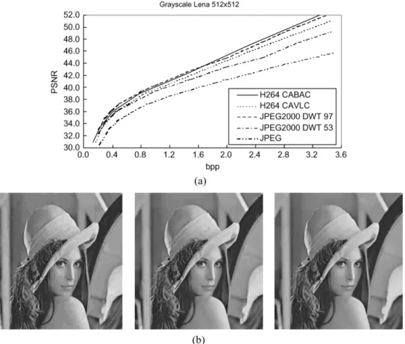
We first compare the compression performance between JPEG, JPEG2000, and H.264/AVC intra frame coder. The results are shown in both objective and subjective manners. Fig. 2(a) is the peak signal-to-noise ratio (PSNR) results under several different bit-rate. The test image is grayscale Lena, and the size is 512 512. Note that because H.264/AVC base-line/main profile only supports 4:2:0 format, we set the chroma components as zero. As can be seen from the rate-distortion curves, the performance of H.264/AVC intra frame coder using context-based adaptive binary arithmetic coding (CABAC) and high complexity mode decision is about the same as that of JPEG2000 using DWT 97 filter, and their performances are 1051-8215/$20.00 © 2005 IEEE
Fig. 1. Core techniques adopted in different image coding standards under the basic coding architecture.
Fig. 2. Comparison between different image coding standards: (a) rate distortion curves and; (b) subjective views at 0.225 bpp (left: JPEG, middle: JPEG 2000 DWT53, right: H.264/AVC I-Frame CAVLC).
the best. H.264/AVC intra frame coder using context-based adaptive variable length coding (CAVLC) and low complexity mode decision is 0.5–1.0 dB worse than JPEG2000 DWT 97, but it is 0.1–1.8 dB better than JPEG2000 DWT 53. The coding performance of JPEG is significantly lower than other standards. Fig. 2(b) shows the subjective views at 0.225 bit/pixel (bpp). The block artifact of JPEG image is very obvious, and the other two images gives acceptable qualities without block artifact. JPEG2000 eliminates the block artifact by adopting DWT while H.264/AVC achieves it by deblocking. The image quality of H.264/AVC is very close to that of
TABLE I
COMPARISON OFCOMPUTATIONALCOMPLEXITY
JPEG2000. Now we compare the computational complexities of the three standards. The instruction profiles are shown in Table I. The test image is 2048 2560 grayscale Bike. The
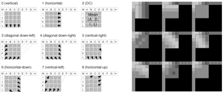
Fig. 3. I4MB; left: illustration of nine 42 4-luma prediction modes; right: examples of real images. ratio of the encoder complexities for JPEG, JPEG2000 (DWT
53), and H.264/AVC intra frame coder (CAVLC and low complexity mode decision), respectively, is about 1:6:6, and the ratio of decoder complexities is about 1:10:2. The encoding complexity of H.264/AVC intracoder is about the same as that of JPEG2000, but the decoding complexity of H.264/AVC is much lower than that of JPEG2000. Moreover, H.264/AVC is a block-based algorithm, which is more hardware-friendly than JPEG2000. DWT is a frame-based transform and thus requires a huge amount of memory. The entropy coder of JPEG2000, embedded block coding with optimized truncation (EBCOT), is a sequential bitplane processing and requires a high operating frequency to meet the real-time constraint. JPEG2000 sequential mode can be replaced by parallel mode (arithmetic coder terminates at the end of each bitplane) in order to decrease the operating frequency with several bit-plane processing engines in parallel, but this may suffer 0.5–1.0-dB quality loss. Thus, for applications whose key functionality is compression instead of scalability, such as digital camera and digital scanner, H.264/AVC intra frame coder may be a more attractive solution. Besides, it can be directly reused for integration of H.264/AVC video coding.
In this paper, two solutions for platform-based design of H.264/AVC intra frame coder are proposed. One is a soft-ware implementation targeted at low-end applications, and the other is a hardware accelerator targeted at high-end appli-cations. The rest of this paper is organized as follows. In Section II, the related background including the flow of mode decision in the reference software is reviewed. Section III describes our fast algorithm. Three speed-up methods are pro-posed. In Section IV, the architecture design of H.264/AVC intra frame coder including reconfigurable predictor genera-tion, transform/inverse transform, quantizagenera-tion, CAVLC, and macroblock pipelining, is discussed. Finally, conclusions are drawn in Section V.
II. FUNDAMENTALS
In this section, technical overview of H.264/AVC intra coding will be introduced.
A. Intraprediction Modes
In H.264/AVC intra coding, two intramacroblock modes are supported. One is intra 4 4 prediction mode, denoted as I4MB, and the other is intra 16 16 prediction mode, denoted as I16MB. For I4MB, each 4 4-luma block can select one of nine prediction modes. In additional to dc prediction, eight directional prediction modes are provided. Fig. 3 shows the illustration of 4 4-luma prediction modes and their examples of intra pre-dictor generation from real image. The 13 boundary pixels from previously coded blocks are used for predictor generation. Fig. 4 shows the illustration of 16 16-luma prediction modes and their real image examples. For I16MB, each 16 16-luma mac-roblock can select one of the four modes. Mode 3 is called plane prediction, which is an approximation of bilinear transform with only integer arithmetic. Chroma intra prediction is independent of-luma. Two chroma components are simultaneously predicted by one mode only. The allowed chroma prediction modes are very similar to those of I16MB except different block size (8 8) and some modifications of dc prediction mode. The mode in-formation of I4MB requires more bits to represent than that of I16MB. I4MB tends to be used for highly textured regions while I16MB tends to be chosen for flat regions.
B. Mode Decision
Mode decision is not specified in H.264/AVC standard. It is left as an encoder issue and is the most important step at the en-coder side because it affects the coding performance most. The reference software of H.264/AVC [8] recommends two kinds of mode decision algorithm, low/high complexity mode deci-sion. Both mode decision methods choose the best macroblock mode by considering a Lagrangian cost function, which includes both distortion and rate. Let the quantization parameter (QP) and the Lagrange parameter (a QP dependent variable) be given. The Lagrangian mode decision for a macroblock proceeds by minimizing
MB
Distortion Rate MB QPP
Fig. 4. I16MB; left: illustration of four 162 16-luma prediction modes; right: examples of real images.
Fig. 5. Left: 1-D 42 4 DCT; middle: 1-D 4 2 4 IDCT; right: 1-D 4 2 4 Hadamard transform/inverse transform.
where the macroblock mode is varied over all possible coding modes. Experimental selection of Lagrangian multipliers is cussed in [9]–[12]. In the low complexity mode decision, dis-tortion is evaluated by sum of absolute differences (SAD) or sum of absolute transformed differences (SATD) between the predictors and original pixels. Usually, the coding performance by selecting SATD is 0.2–0.5 dB better. The rate is estimated by the number of bits required to code the mode information. In the high complexity mode decision, distortion is evaluated by sum of square differences (SSD) between the original samples and the reconstructed pixels (original pixels plus prediction residues after DCT/Q/IQ/IDCT). The rate is estimated by the number of bits required to code the mode information and the residue. The high complexity mode decision method is less suitable for real-time applications. The high complexity mode requires the most computation but leads to the best performance. Note that when processing I4MB, DCT/Q/IQ/IDCT must be performed right after a 4 4-block is mode decided in order to get the re-constructed boundary pixels as the predictors of the following 4 4-blocks.
C. Transform and Quantization
H.264/AVC still adopts transform coding for the prediction error signals. The block size is chosen as 4 4 instead of 8 8. The 4 4 DCT is an integer approximation of original floating point DCT transform. An additional 2 2 transform is applied to the four dc-coefficients of each chroma component. If a-luma macroblock is coded as I16MB, two dimensional (2-D) 4 4 Hadamard transform will be further applied on the 16 dc coeffi-cients of-luma blocks. Fig. 5 shows the matrix representation
for 4 4 one-dimensional (1-D) DCT, IDCT, and Hadamard transform. Note that due to the orthogonal property and diag-onal symmetry, the inverse Hadamard transform is the same as its forward one. The scaling of the transform is combined with quantization. H.264/AVC uses scalar quantization without dead-zone. The quantization parameter QP ranges from 0 to 51. An increase in QP approximately reduces 12.5% of the bit-rate. The quantized transform coefficients of a block are scanned in a zigzag fashion. The decoding process can be realized with only additions and shifting operations in 16-b arithmetic. For more details, please refer to [13].
D. Entropy Coding
In H.264/AVC, two entropy coding schemes are supported. One is VLC-based coding, and the other is arithmetic coding [14]. In this subsection, VLC-based coding will be introduced. In the baseline profile, a single infinite-extension codeword set (Exp-Golomb code) is used for all syntax elements except the quantized transform coefficients. Thus, instead of designing a different VLC table for each syntax element, only a mapping to the single codeword table is customized according to the data statistics. For transmitting the quantized transform coefficients, a more sophisticated method called context-based adaptive variable length coding (CAVLC) is employed. In this scheme, VLC tables for various syntax elements are dependent on previous symbols. Since the VLC tables are well designed to match the corresponding conditioned symbol statistics, the entropy coding performance is improved in comparison to schemes using a single fixed VLC table. Let us take Fig. 6 as an example of coding a 4 4-block by CAVLC. At first,
Fig. 6. Example of encoding a 42 4-block by CAVLC.
Fig. 7. Instruction profile of H.264/AVC Baseline Profile intra frame coder with low complexity mode decision for 7202 480 4:2:0 30-Hz Video (QP = 30).
the 4 4-block is backward zigzag scanned. The number of total nonzero coefficients and the number of tailing ones are transmitted as a joint symbol. The following symbols are signs of trailing ones, levels, number of total zeros before the last nonzero coefficient, and runs before nonzero coefficients. Each symbol has corresponding context-based adaptive VLC tables. The decoding process is shown at the right side. Note that run information of a level is not transmitted for the last nonzero coefficient or when the total runs have reached the number of total zeros before the last nonzero coefficient as shown in the example.
III. FASTALGORITHM
In this section, a fast algorithm for software implementation will be described according to our analysis. The proposed com-plexity reduction methods are simple and effective.
A. Analysis of Computational Complexity
The instruction profile of H.264/AVC Baseline Profile intra frame coder with low complexity mode decision for SDTV specification (720 480 4:2:0 30 Hz) is shown in Fig. 7. Real-time processing requires 10829 million instructions per second (MIPS), which is far beyond the capability of today’s general purpose processor (GPP). The instructions are classified as three categories: computing, controlling, and memory access. It is shown that memory access operations are the most highly demanded. This reveals that for DSP-based implementation, the speed of DRAM and the size of cache affect the performance considerably, and for ASIC-based accelerator, local SRAMs and registers are critical to reduce the bus bandwidth. Fig. 8
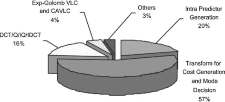
Fig. 8. Run-time percentages of various functional modules.
shows the run-time percentages of several major functional modules. As can be seen, transform for cost generation (SATD computation) and mode decision take the largest portion of computation, and intra predictor generation is the second. These two functions take 77% of computation and obviously are the processing bottleneck of the H.264/AVC intra frame coder. This result is quite reasonable because intra prediction has to generate 13 kinds of different predictors for each-luma sample and 4 kinds for each chroma sample. Also, the residues of each prediction mode also need to be 2-D Hadamard trans-formed into cost value for accumulation. After mode decision, only the decided modes and its corresponding residues are processed by DCT/Hadamard transform, quantization, inverse quantization, inverse DCT/Hadamard transform, and entropy coding. Exp-Golomb VLC and CAVLC are bit-level processing with complex controlling, but their computational load is not very large. Note that the run-time percentage of CAVLC will vary according to different QP values.
B. Analysis of Computation Reduction Techniques
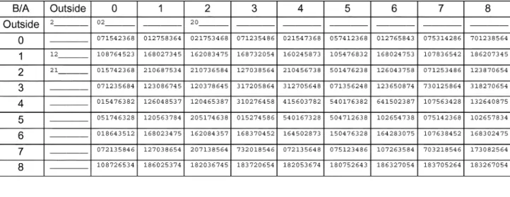
As mentioned before, there are nine prediction modes for I4MB, and their numbers are shown in Fig. 3. Statistically, the smaller the number is, the more possible the mode will occur. Thus, this global statistics of I4MB modes can be used to save computation by searching only some modes with smaller numbers. How many modes should be searched is a tradeoff between computation and image quality. Clearly, global statistics cannot reflect the correlation of local modes. It may suffer severe PSNR degradation. Therefore, we tried a context-based approach considering the local statistics of neighboring blocks. Table II lists the most probable I4MB mode followed by other modes with gradually decreasing possibilities when the left and top neighboring 4 4-blocks are given. This is obtained by modifying the previous version of Working Draft [15]. Mode decision process can be accelerated
TABLE II
CONTEXT-BASEDMOSTPROBABLEMODES
Fig. 9. Subsampled pixels in a 42 4-block: left: pattern one and right: pattern two.
by searching only a few modes with higher possibilities. This method somewhat improves the quality of previous method but still suffers considerable PSNR loss compared with full search. This is caused by error propagation. When a block chooses a suboptimal mode instead of optimal mode, it will affect its following right and bottom blocks. Thus, we should find a way to detect the suboptimal modes and prevent them from propagating too far to make the neighboring blocks fail to find the best mode. Our improvement will be shown in the next subsection.
Single instruction multiple data (SIMD) is common in today’s GPP and DSP. We can reduce the computation by reducing the data bit-width. For example, Philips TriMedia [16] is a 32-b VLIW/SIMD multimedia processor. Each of the five issue slots can simultaneously process two 16-b data or four 8-b data. The difference between original 8-b pixel and its predictor requires 9-b representation, which is over 8 b, so we can compute two differences in parallel. If the pixel bit-width is reduced to 7 b, the difference value can be represented within 8 b. In this way, four differences can be computed at the same cycle in one issue slot. Although the speed is doubled, some degradation of image quality may occur. Bit-width reduction can be also utilized in hardware design to save area and power as long as the PSNR drop can be tolerated.
Simplification of matching operations is also utilized. In-tramode decision requires generation of predictor and difference operation for each pixel, and 2-D 4 4 Hadamard transform for blocks to compute SATD. If the pixels are subsampled by two, 50% of computation can be reduced. The subsampled patterns are shown in Fig. 9. Given a prediction mode, originally 16 prediction pixels have to be generated, 16 difference operations have to be performed, and the SATD has to be computed.
Now only eight prediction pixels have to be generated, and only eight difference operations have to be performed for each 4 4-block. As for the SATD computation, if we replace the omitted pixels by zero, 50% of computation reduction cannot be attained. The definition of SATD of a 4 4-block is defined in Fig. 10. There are 48 (3 16) addition operations in the horizontal transform, 48 addition operations in the vertical transform, 16 absolute value operations, 15 additions in accu-mulation, and one shift operation. Replacing the omitted pixels by zero, as shown in Fig. 11, requires 16 addition operations in the horizontal transform, 48 addition operations in the vertical transform, 16 absolute value operations, 15 additions in accu-mulation, and one shift operation. The number of operations is reduced from 128 to 96. Only 25% of the SATD computation is reduced. What is more, replacing the omitted pixels by zero will enhance the high frequency components, which will affect the result of mode decision. Therefore, we replace the omitted pixels by its neighboring pixels, as shown in Fig. 12. In this way, only 24 addition operations are required in the horizontal transform because the result of the first column will be exactly the same as the second column, and the third will also be the same as the fourth. In the vertical transform, only 24 addition operations are required because the output of the third and fourth columns are all zero. Since there are only eight nonzero terms, only eight absolute value operations, seven addition operations, and one shift operation are further executed to get the SATD. The total number of operations becomes 64, and percentage of complexity reduction for SATD computation is also 50%.
C. Proposed Algorithm
In this subsection, a fast algorithm for H.264/AVC intracoder is proposed based on the reduction techniques previously discussed. First, no matter the intramacroblock mode is I4MB or I16MB, the computation of Lagrangian cost for each 4 4-block is performed under subsampled resolution by using pattern one shown in Fig. 9. Second, it was mentioned in the previous subsection that the context-based skipping of unlikely candidates for I4MB suffers from error propagation problem. We propose two techniques to handle this problem, periodic
Fig. 10. Original definition of SATD for a 42 4-block.
Fig. 11. Replacing the subsampled pixels by zero.
insertion of full-search 4 4-block and adaptive threshold on the distortion. As shown in Fig. 13, stands for a full search 4 4-block, and stands for a partial search 4 4-block. In an 8 8-block, the top left 4 4-block adopts full search while the other three 4 4-blocks utilize context-based partial search stated in the previous subsection. In this way, we can stop propagating the error too far. How long the period should be depends upon the tradeoff between computation and image quality. The three partial search blocks in an 8 8-block may
still miss the optimal modes. In these cases, the SATD values of these partial search blocks are much larger than the corre-sponding full search block. Therefore, we apply an adaptive local threshold on the minimum SATD of partial search blocks. If the minimum SATD of a partial search block is too large, rest I4MB modes still need to be searched. The threshold is defined as follows:
Fig. 12. Proposed SATD for subsampling.
Fig. 13. Corresponding positions between full search blocks and partial search blocks for I4MB.
where MinSATD denotes the minimum SATD of the top left full search 4 4-block in an 8 8-block. In this way, the threshold is adaptive to local statistics of the image. Also, , a constant scalar, is set as 2.0 in our algorithm and can be used as a tradeoff between computation and image quality. Theoret-ically, the average saved computation is stated as follows: Computation
AvgSearched
% (3)
where Computation is percentage of saved computation for intra prediction and mode decision, and AvgSearchedI4MB denotes the average number of searched I4MB modes. As mentioned before, there are nine, four, and four modes for I4MB, I16MB, and chroma intra prediction, respectively. Since the number of chroma pixels is half of the number of-luma pixels, the ratio of their computational complexities is 9:4:2. The factor is due to subsampling by two.
TABLE III SAVEDCOMPUTATION
D. Experimental Results
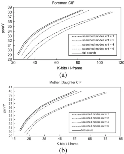
Table III shows the experimental results of average saved computation for intra prediction and mode decision. Eight stan-dard sequences were tested with many QP values. As can be seen, the average saved computation is about 60%. According to the previous analysis, intra prediction and mode decision take 77% of the total computation of H.264/AVC intra frame coder. Therefore, the proposed fast algorithm can reduce 45% of the total complexity. Subsampling contributes most to the computation reduction while context-based skipping of unlikely I4MB candidates with periodic insertion of full search blocks and adaptive threshold checking can further reduce more com-putation with little quality loss. Fig. 14 shows the rate-distor-tion curves under different numbers of searched I4MB modes using context-based skipping of unlikely candidates without in-sertion of full-search blocks. The PSNR degradation is very se-vere when the number of searched I4MB modes is equal or less than two. Performance of searching one I4MB mode is even better than searching two I4MB modes. This is because
Fig. 14. Rate-distortion curves under different numbers of searched I4MB modes using context-based skipping of unlikely candidates for CIF videos. (a) Foreman. (b) Mother and Daughter.
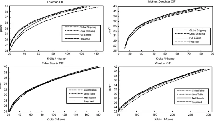
searching one mode happens to select mode two (dc predic-tion) for all the 4 4-luma blocks in a frame, and searching two modes suffers from severe error propagation. By experi-mental results, searching the most possible four I4MB candi-dates, which is finally used in our experiments, is a reasonable choice to avoid too much loss of image quality. We did not use pixel bit-width truncation in our simulation because it is platform dependent. The rate-distortion curves of our final al-gorithm are illustrated in Fig. 15. Four sequences are shown. The other four sequences show the same trend and are omitted due to the limited spaces. The PSNR drop of the proposed al-gorithm is less than 0.3 dB in all sequences. Subsampling and searching only four globally most possible I4MB modes (mode 0–3) or four locally (context-based) most possible modes shows a significant loss of image quality, which indicates that periodic insertion of full search blocks effectively improves the image quality while subsampling together with context-based partial search greatly decreases complexity.
IV. HARDWAREARCHITECTURE
In this section, a parallel H.264/AVC intra frame coding ar-chitecture with efficient macroblock pipelining is proposed for SDTV specification (720 480 4:2:0 30-Hz video), which re-quires to encode about 16 Mega-pixels within one cycle. The
implemented algorithm is the same as the reference software except that Hadamard-based mode decision is changed to DCT-based. The detailed analysis and system/module designs are de-scribed in the following subsections.
A. Exploration of Parallelism
From the complexity analysis in Section III, it is known that intra prediction and mode decision place the heaviest compu-tational load on processor. Parallel architecture is urgently de-manded to accelerate this critical function. In this subsection, we will analyze the H.264/AVC intra prediction algorithm to obtain the most suitable degree of parallelism required for intra prediction and mode decision to meet the SDTV specification. Because transform for Lagrangian cost generation (SATD com-putation) is highly dependent on intra predictor generation and must be performed right after intra predictor generation, the par-allelism of intra prediction unit should be the same as the trans-formation unit. Thus, we start the exploration of parallelism from intra predictor generation.
First, two assumptions are made. One is that a reduced in-struction set computer (RISC) is able to execute one inin-struction in one cycle with an exception of multiplication requiring two cycles, and the other is that a processing element (PE) is ca-pable of generating the predictor of one pixel in one cycle. Next,
Fig. 15. Rate-distortion curves of proposed algorithm (subsampling+ context-based partial search + periodic insertion of full search + adaptive SATD threshold) compared with full search, global method (subsampling+ partial search utilizing global statistics), and local method (subsampling + context-based partial search).
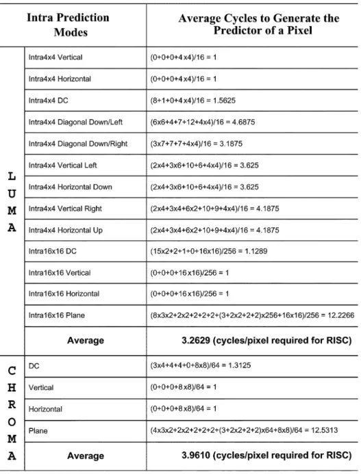
we compute the average instruction counts required for intra predictor generation. The instructions includes arithmetic com-puting and data transfer from memory unit to execution unit. For example, the operation “ ” requires two load in-structions and one add instruction. The actual instruction count for RISC is higher than the provided data because the address generation (AG) is excluded for two reasons. For software im-plementations, different coding styles and compilers will lead to very different results. On the hardware accelerator, AG be-longs to controlling circuits, which usually occupy a very small portion of chip area, and it has nothing to do with the design of intra predictor generation. Table IV shows the analysis of in-structions for intra predictor generation. I16MB plane predic-tion mode demands the most cycles than other predicpredic-tion modes because two multiplication operations are required for one pixel. Detailed explanation is omitted for simplicity, and interested readers can refer to [1] for checking. In sum, we conclude that it takes 3.2629 and 3.9610 cycles for a RISC to generate one-luma predictor and one chroma predictor, respectively, in average.
To design the hardware architecture of intra predictor genera-tion unit, we first bring up three possible solugenera-tions, as shown in Fig. 16. The first one is a RISC solution. In the era of system on chip, embedded RISC becomes essential in chip design. How-ever, the RISC must work at the frequency higher than 521.9 MHz to meet the real-time requirement of SDTV specification. Consequently, RISC implementation seems to be impractical, not to mention transform, entropy coding, and other system jobs such as real-time operation system (RTOS), camera control, net-work, and others. The second possible solution is a set of ded-icated hardware PEs for intra predictor generation. Suppose 13
kinds of PE are developed, and each one is dedicated for one kind of intra prediction mode. The hardware can generate 13 kinds of-luma predictors or four kinds of chroma predictors in one cycle. The architecture only needs to operate at 15.6 MHz under our specification. However, this solution does not con-sider the correlation between different prediction modes and has high hardware cost. The third choice is to design a recon-figurable PE to generate all the intra predictors with different configurations. This solution targets at higher area-speed ef-ficiency. Nevertheless, implementation of a reconfigurable PE is not straightforward. It requires several design techniques to reach resource sharing. Moreover, reconfigurable PE still re-quires to operate at 202.2 MHz to meet our target. For these reasons, parallel reconfigurable PEs become the most promising solution. Table V lists the hardware complexity and required fre-quency of the three solutions under different degrees of paral-lelism. Although the assumption that the hardware complexity of one PE is similar to those of RISC and one dedicated PE is quite rough, it is still proper to reflect the fact that RISC is too slow, dedicated PEs are too expensive, and reconfigurable PE is a good tradeoff between area and speed. Finally, we conclude this subsection by adopting four-parallel reconfigurable PE for intra predictor generation in our design.
B. Initial System Architecture
In conventional video coding standards, prediction engine and block engine (DCT/Q/IQ/IDCT/VLC) can be clearly sepa-rated. After prediction engine finishes processing a macroblock, block engine takes over this macroblock, and prediction engine goes on processing the next macroblock. However, H.264/AVC
TABLE IV
ANALYSIS OFINSTRUCTIONS FORINTRAPREDICTORGENERATION
utilizes intra prediction in the spatial domain, which destroys the traditional macroblock pipelining. After prediction of a macroblock and before corresponding reconstructed pixels at the output of the DCT/Q/IQ/IDCT loop are produced, next macroblock cannot be predicted. The situation is even worse for I4MB prediction modes. Prediction and mode decision of a 4 4-block cannot be performed until the previous 4 4-block is reconstructed. If the number of processing cycles for DCT/Q/IQ/IDCT loop is too large, prediction circuits must be stalled to wait for reconstruction, and the hardware utilization will be significantly decreased.
We divide our system into two main parts, the encoding loop and the bitstream generation unit, as illustrated in Fig. 17. The
system block diagram is shown in the upper part while the pro-cessing schedule is in the bottom part. First, the system encodes a frame macroblock by macroblock in progressive order, and we buffer one row of reconstructed pixels (720-luma pixels and 360 2 chroma pixels) in the external DRAM. At the beginning of a macroblock, current macroblock pixels
and upper reconstructed pixels (17) are loaded from external DRAM to on-chip SRAM. The reconstructed pixels of the previous (left) macroblock can be directly kept in registers to save bus bandwidth. Assume the bus bit-width is 32, loading data requires 101 cycles. The initialization of a macroblock also includes loading of some coding information from neighboring macroblocks (intra prediction modes and number of nonzero
Fig. 16. Three possible solutions and the required working frequency to meet the real-time requirement of SDTV specification.
TABLE V
HARDWARECOMPLEXITY ANDOPERATINGFREQUENCY FORINTRAPREDICTORGENERATION
coefficients) on the upper row for entropy coding. The coding information of the left macroblock can be also saved in reg-isters for entropy coding of current macroblock. With on-chip SRAM, the bus bandwidth is reduced from hundreds of MB to about 20 MB/s. Among the data transfer between external DRAM and our accelerator, the input pixel rate contributes to 15.55 MB/s (720 480 1.5 30), the output data rate ranges from 5% to 20% of the input pixel rate, saving, and loading of reconstructed pixels of upper rows requires 2.6 MB/s
, and the data amount of coding infor-mation is very small. Then, we start the intra prediction block by block. According to the analysis in Subsection IV.A, given a 4 4-luma block and a prediction mode, four pixels are re-quired to be processed (predictor generation and transform) in one cycle. Therefore, the number of cycles required for-luma
intra prediction and mode decision is , and
that for chroma is . As previously discussed, before DCT/Q/IQ/IDCT finishes the previous 4 4-block, cur-rent 4 4-block cannot proceed to intra prediction, so the re-quired time for intra prediction is actually longer. We intended to adopt two-parallel architectures for DCT/Q/IQ/IDCT. How-ever, Four-parallel transform unit doubles the speed of two-par-allel transform unit with only a little area overhead (discussed in Section IV-G), so four-parallel DCT/IDCT is adopted at last. CAVLC is a sequential algorithm and its computational loading
is not very large. Hence, parallel processing is not a must. In sum, the initial system architecture needs about 2400 cycles to encode one macroblock. Also, with the straightforward data flow, the residues are generated twice. One time is used for intra predictor generation and mode decision while the other is for entropy coding of the best mode. On-chip memory access is 113.17 MB/s.
C. System Architecture With Macroblock Pipelining
In the previous subsection, it is observed that the number of processing cycles for encoding loop is about the same as that for bitstream generation unit in the worst case. These two pro-cedures are separable because there is no feedback loop be-tween them. Therefore, a task-level interleaving scheme, i.e., macroblock pipelining, is incorporated into our design to accel-erate the processing speed at the cost of coefficient buffer for a macroblock, as illustrated in Fig. 18. The data flow is the same with that of initial system architecture except the two stages process different macroblocks. After intra prediction and mode decision, the residues are generated again, sent to DCT/Q, and stored in the coefficient buffer. The buffer is composed of four memory banks, and the size of each bank is 96 words by 16 b. The buffer is indispensable for macroblock pipelining. When current macroblock is processed by encoding loop, CAVLC pro-cesses previous macroblock simultaneously. The bus bandwidth
Fig. 17. Illustration of initial system architecture.
and the amount of on-chip memory access are still the same as before while the processing throughput is reduced to less than 1300 cycles/macroblock.
D. System Architecture With DCT-Based Mode Decision
In the H.264/AVC reference software, Hadamard transform is involved in generating cost for mode decision. The quan-tized transform coefficients in the mode decision phase cannot be reused for CAVLC. Thus, we modify the mode decision algorithm by using DCT instead of Hadamard transform to generate Lagrangian costs so that the transform coefficients can be reused. Luma mode decision is performed block by block, and 13 kinds of predictors are generated for each 4 4-block. The former nine prediction modes decide the best I4MB mode, and the quantized transform coefficients will be stored in the coefficient buffer right after mode decision and reconstruction of a 4 4-block. In this way, if I4MB mode is better than I16 MB, re-generation of-luma quantized transform residues can be avoided. The improvement will be significant in high quality applications for almost all macroblocks select I4MB. In our experience, when QP is smaller than 25, the percentage of I16MB mode is less than 10%. The amount of on-chip memory access can thus be reduced from 113.17 to 72.25 MB/s. Also, the proposed mode decision does not suffer any quality loss compared with the mode decision in the reference software. Fig. 19 shows the final system block diagram of our proposed H.264/AVC intra frame encoder. The system is partitioned into three independently-controlled parts: forward encoding part,
backward reconstruction part, and bitstream generation part. The system buffers one row of reconstructed pixels and one row of coding information at the external DRAM. The coding information includes I4MB modes for most probable mode prediction, number of nonzero coefficients for CAVLC. The external DRAM size is proportional to the width of image.
E. Evaluation of System Performance
Table VI shows the comparison of the three developed archi-tectures. The first version is a parallelism optimized architecture with straightforward data flow design and Hadamard-based mode decision. The second architecture evolves from the first version by considering macroblock pipelining. The third version replaces the Hadamard-based mode decision by DCT-based mode decision. We can see from the table that the last version has the fewest processing cycles and the least memory access. Compared with software implementation on RISC, which requires 0.28 M cycles to encode one macroblock, the performance of proposed architecture is 215.4 times faster than the software implementation. The chip only needs to operate at about 50 MHz to meet the SDTV specification.
F. Intra Predictor Generation Unit
In this subsection, a reconfigurable intra predictor generator to support all of the prediction modes will be discussed. The pro-posed hardware is a four-parallel architecture to meet the target specification. Four predicted pixels are generated in one cycle
Fig. 18. Illustration of system architecture with proposed macroblock pipelining.
except for the most complicated prediction mode, I16MB plane prediction mode. We will introduce a decomposition technique to reduce the complexity of PE. Before entering the following subsections, please recall the analysis in Table V. Four recon-figurable PEs will be used to generate 4 1 predictors in one cycle.
1) I4MB Prediction Modes: I4MB prediction is arranged in
a three-loop fashion. The outer loop is the 16 4 4-luma blocks, the middle loop is the nine I4MB modes, and the inner loop is the four rows of 4 1 pixels in a block. Totally
cycles are required to generate all kinds of I4MB predictors for a whole macroblock, and a row of 4 1 pixels is predicted in one cycle. Frequent access of neighboring reconstructed pixels (A-H and I-M shown in Fig. 3) is inevitable, so we buffer these pixels in registers and update the registers before starting I4MB prediction of a 4 4-block, as corresponded with the “Decoded Block Boundary Handle” (DBBH) in Fig. 19. Let us denote the top left, top right, bottom left, and bottom right positions of a 4 4-block as (0, 0), (0, 3), (3, 0), and (3, 3), respectively. The detailed definitions of I4MB predictors are shown in Table VII. For example, diagonal down-left type predictor at position (0, 0)
is . Except for dc mode, only three or
fewer neighboring reconstructed pixels are involved in the gen-eration of a predictor, and two 8-b adders, one 9-b adder, and one
rounding adder (four adders in total) are required to generate a predictor in one cycle. Multiplexers are required to select proper neighboring reconstructed pixels. The selection can be viewed as a sliding window (3 1 pixels) shifting between “LKJ” to “FGH.” If we want to generate the dc predictor in one cycle, the required circuits will expand to four 8-b adders, two 9-b adders, one 10-b adder, and one rounding adder, and the utilization of the extra two 8-b adders, one 9-b adder, and one 10-b adder will be extremely low for they are only useful when dc mode is in process. For a single PE design, it is better to compute the dc predictor using more cycles with fewer adders and save the dc value in the register for later reuse. As for a four-parallel design, since the dc mode has the same predictors at all positions, four PEs can be joined together to compute the dc predictor in one cycle.
2) I16MB Prediction Modes: The predictors of I16MB
ver-tical mode and horizontal mode can be directly acquired from the neighboring reconstructed pixels by DBBH. Like I4MB dc predictor, I16MB dc predictor can be calculated in several cy-cles by few adders. The detailed definition of I16MB plane pre-diction mode, which is an approximation of bilinear transform, is described in the following:
Fig. 19. Illustration of final system architecture.
TABLE VI
COMPARISON OFSYSTEMARCHITECTURES
(5) (6) (7) (8)
(9)
where denotes the position ([0, 0], [0, 15], [15, 0], and [15, 15] are the top left, top right, bottom left, and bottom right of a-luma macroblock, respectively), represents the neigh-boring reconstructed pixel value, Pred indicates the generated predictor value, and Clip1 is to clip the result between 0 and
255. Fig. 20 may help understand I16MB plane prediction mode better. As shown in (4), two multiplications, five additions, and one shift are required. Assume we are going to reuse those adders, which were planned to generate one I4MB predictor in one cycle, to produce one I16MB plane predictor, it is obvious that the required processing cycles will be quite longer. Besides, the control signals of the multiplexers for selecting adder in-puts will be very complex. Therefore, we propose a more ef-ficient method to decompose plane predictors by using only accumulation operation. Firstly, for each 16 16-luma mac-roblock, there will be a short setup period to find the values of , and and buffer them in registers. The multi-plications in (8) and (9) can be replaced by additions as fol-lows. For example, when
TABLE VII
DEFINITIONS OFI4MB PREDICTORS
three times. In our implementation, sev-eral extra adders are used to compute , and to
re-duce the complexities of reconfigurable PEs and control sig-nals. After a short time of setup, we compute four seed values,
Fig. 20. Illustration of I16MB plane prediction mode.
Fig. 21. Decomposition of I16MB plane prediction mode.
TABLE VIII
COMPARISONBETWEENDIRECT ANDDECOMPOSITION FORPLANEPREDICTION
, and . With the pre-computed , and these seed values, all the other I16MB plane predictors can be computed by add and shift operations. As ex-pressed in Fig. 21, , and are the seed values of the
columns – – – , and – ,
respec-tively. For example, when is obtained, ,
and can be computed from adding with , and
, respectively, by different PEs simultaneously. Next, the re-sults on the first row can be added with to calculate the next four predictors on the second row in parallel by the four PEs. The same process goes on until the bottom of macroblock is reached, and the four columns of predictors are all generated. The comparison of hardware resources and the required computing cycles are shown in Table VIII. Clearly, plane decomposition method is more effi-cient than direct implementation in both aspects. The chroma prediction is similar to I16MB and can be derived by analogy.
3) Interleaved I4MB/I16MB Prediction Schedule: In fact,
the sequential processing of I16MB after I4MB as shown in Fig. 18 will cause a data dependency problem for I4MB. As stated before, a new 4 4-block cannot be predicted before reconstruction of previous 4 4-block, so the cycles required for I4MB prediction may be longer than 576. Although par-allel Q/IQ/IDCT have been implemented as shown in 19, when the best I4MB mode of a 4 4-block is determined as one of the last two modes (vertical left or horizontal up), Q/IQ/IDCT still cannot complete the reconstruction in time to avoid the bubble cycles for “Intrapredictor Generation”/DIFF/DCT be-fore starting prediction of the next 4 4-block. In order to avoid these bubble cycles, I16MB prediction is inserted right after I4MB prediction for the same 4 4-block so that Q/IQ/IDCT can finish in time, as shown in Fig. 22. However, dc coefficients of the four I16MB modes have to be stored in registers because the distortion cost of I16MB modes in the reference software requires to further apply 4 4 2-D Hadamard transform on the 16 dc values. This is a tradeoff between speed and area.
4) Reconfigurable Intra Predictor Generator: Based on
the analysis in previous subsections, the hardware architecture of our four-parallel reconfigurable intra predictor generator is shown in Fig. 23, which includes the sliding window selection
Fig. 22. Illustration of interleaved I4MB/I16MB prediction at 42 4-block level.
Fig. 23. Proposed four-parallel reconfigurable intra predictor generator.
circuits for I4MB and for decomposition of I16MB plane prediction. The inputs of the generator are the neighboring reconstructed pixel provided by DBBH module. The recon-figurable architecture can support all kinds of intra prediction modes in H.264/AVC with different configurations.
First, I4MB/I16MB horizontal/vertical mode simply selects the “bypass” data path. Second, multiple PEs are involved in generating I4MB/I16MB/chroma dc predictor. For I4MB dc mode, sum of “ABCD” is computed by the second PE, sum of “IJKL” is computed by the third PE, and their
out-puts are fetched to the first PE to get the final dc value in one cycle. Chroma dc mode is done in a similar way. As for I16MB dc predictor, it takes four cycles. The configuration for I16MB dc mode is shown in Fig. 24. Let us denote the top reconstructed pixels and the left reconstructed pixels as T00–T15 and L00–L15, respectively. It takes three cy-cles for PE0-PE3 to accumulate eight reconstructed pixels.
For example, PE0 computes “ ,”
“ ,” and
Fig. 24. Configuration of I16MB dc mode.
Fig. 25. Configuration of I4MB directional modes 3–8.
at the first three cycles, respectively. At the fourth cycle, the results of four PEs are fetched to PE0 to generate the final dc value.
Fig. 25 shows the configuration for I4MB directional modes 3–8. For example, to interpolate the I4MB diagonal down-left predictors of the first row, The first, second, third, and fourth PE
Fig. 26. Configuration of I16MB plane prediction mode.
Fig. 27. Fast algorithms for (left) DCT, (middle) IDCT, and (right) Hadamard transform. should select “ABC,” “BCD,” “CDE,” and “DEF,” respectively.
The rest I4MB directional predictions are similar.
Fig. 26 shows the configuration of I16MB plane prediction mode. Assume now we are going to generate the predictors of the first four columns – . After “A0” is computed during initial setup, to generate the four predictors of the first row, the four inputs of the adders at PE0-PE3 are (A0, 0, 0, 0), (A0, b, 0, 0), (A0, b, b, 0), and (A0, b, b, b), respectively. To generate the predictors of the following rows, the four inputs of the adders at each PE are configured as the output of “D” reg-ister, 0, 0, and “c.”
G. Multitransform Engine
The matrix representations of 1-D 4 4 DCT, IDCT, Hadamard transform are shown in Fig. 5. Their fast algorithms are shown in Fig. 27. The matrices only contain six coefficients,
, which can be implemented by shifters and adders. The fast algorithms further reduce the number of addition from 16 to eight with butterfly operations. Because the three transforms have the same butterfly structure, we can merge them into a multiple function transform unit as shown in Fig. 28. Multiplexers are required to choose proper coefficients for different transforms.
Fig. 29 is the proposed parallel architecture. It contains two 1-D transform units and transpose registers. The 1-D transform unit is implemented as the butterflies. Since the butterflies only contain shifts and adds, the 1-D modules are designed to com-plete the transform within one cycle. The data path of the trans-pose registers can be configured as leftward, downward, and stall. The latency of the 2-D transform is four cycles. Block pixels are inputted row by row. The output enable signal is prop-agated or stalled with the data enable signal at the input. From
Fig. 28. Overlapped data flow of the three fast algorithms.
Fig. 29. Hardware architecture of multitransform engine.
the beginning, the pixels in the first 4 4-block are fetched and transformed row by row, and the data path of the transpose regis-ters is configured as downward. After four cycles, the horizontal transform results are all buffered in the transpose registers. Next, the data path is changed to leftward. We keep on fetching the row data of the second 4 4-block to perform the horizontal transform. At the same time, the vertical transform for the first block is also performed. When the first block is finished, the hor-izontal transform results of the second block are in the transpose registers. Next we change the data path to downward and go on processing the vertical transform of the second 4 4-block and the horizontal transform of the third 4 4-block. In this way, the hardware utilization is 100%.
Table IX shows the synthesized results with Avant! 0.35- m cell library. The critical path of single transform is about 8 ns, and the critical path for multiple transforms or conventional serial architecture with single transform is about 12 ns. The gate counts of proposed parallel architectures range from 3.7 to 6.5 K. The conventional architecture for forward transform requires 3.6 K gates and an extra SRAM. The gate count of our parallel forward transform architecture is about the same as that of conventional serial forward transform architecture. However, the processing capability of parallel architecture is five times of serial one. The main reason is that the transform matrices are very simple. The area of the four-parallel 1-D transform is about
four times larger than that of serial, but the transpose registers, which are necessary for both serial and parallel architectures, dominate the total area of the 2-D transform circuits. Interested readers can refer to [17] for more details.
H. Bitstream Generation
Fig. 30 shows the proposed sequential architecture for bit-stream generation. The macroblock header is first produced and sent to the packer. Then, the CAVLC forms bitstream block by block. It takes 16 cycles for the address generator to load coeffi-cients of a 4 4-block from the memory in a reverse zigzag scan order. During the loading process, the level detection checks if the coefficient is zero or not. If the level is nonzero, it will be stored into the level-first-in first-out buffer (FIFO), and the corresponding run information will also be stored to the run-FIFO. At the same time, the trailing one counter, total coef-ficient counter, and run counter will update the corresponding counts into registers. After 16 cycles of the scan operation, the total coefficient/trailing one module will output the code word to packer by looking up the VLC table according to the results of total coefficient register and trailing one register. Next, level code information is sent to the packer by looking up the VLC table for levels. The selection of table is according to the mag-nitude of level. Finally, total zero and runs are encoded also by looking up table according to the results of registers.
The level table of CAVLC has a maximum codeword length of 32-b, so we designed a 32-b packer, as shown in Fig. 31. The inputs of the packer are a 32-b codeword and a five-bits codelength. The left side of the packer is to pack the codewords to two ping-pong 32-b buffers while the right side computes the remainder length of the 32-b buffers. When one of the 32-b buffers is full, the “OE” signal will be enabled. For more details, please refer to [18].
I. Implementation
A prototype chip is implemented to verify the proposed VLSI architecture for H.264/AVC intra coding. The chip photo and specifications are shown in Fig. 32. The gate count of each func-tional block is listed in Table X. Seven SRAM modules are used in the chip. One 64 32 RAM is to buffer the I16MB plane pre-dictors so that they do not have to be generated again when se-lected as the final macroblock mode. Two 96 32 RAMs are used to save current macroblock and reconstructed macroblock. The other four RAMs are used as quantized transform coeffi-cient buffer for macroblock pipelining.
V. CONCLUSION
In this paper, we contributed a fast algorithm and a VLSI architecture for H.264/AVC intra frame coder. Our algorithm includes context-based adaptive skipping of unlikely predic-tion modes, simplificapredic-tion of matching operapredic-tions, and pixel truncation to speed up the encoding process. Periodic insertion of full search blocks effectively prevents the quality degrada-tion. About half of the encoding time can be saved while the maximum PSNR loss is less than 0.3 dB. As for the hardware architecture part, at first we analyzed the intra coding algorithm
TABLE IX
SYNTHESIZEDRESULTS OFPARALLEL ANDSERIALTRANSFORMARCHITECTURES
Fig. 30. Hardware architecture of bitstream generation engine.
Fig. 31. Hardware architecture of the 32-b packer.
by using a RISC model to obtain the proper parallelism of the architecture under SDTV specification. Secondly, a two-stage macroblock pipelining was proposed to double the processing capability and hardware utilization. Third, Hadamard-based mode decision was modified as DCT-based version to reduce
40% of the memory access. Our system architecture is 215 times faster than RISC-based software implementation in terms of processing cycles. In addition, we also made a lot of efforts on module designs. Reconfigurable intra predictor generator can support all of the 17 kinds of prediction modes
Fig. 32. Chip photograph and specifications.
TABLE X GATECOUNTPROFILE
including the most complex plane prediction mode, which is solved by a decomposition technique. Parallel multitransform architecture has four times throughput of the serial one with only a little area overhead. CAVLC engine efficiently provides the coding information required for the bitstream packer. A prototype chip was fabricated with TSMC 0.25- m comple-mentary metal–oxide–semiconductor (CMOS) 1P5M process and is capable of encoding 16 Mega-pixels within one cycle, or encoding 720 480 4:2:0 30 Hz video in real time at the working frequency of 54 MHz. The transistor count is 429 K, and the core size is only 1.855 1.885 mm .
REFERENCES
[1] Draft ITU-T Recommendation and Final Draft International Standard
of Joint Video Specification, May 2003. Joint Video Team.
[2] Information Technology—Coding of Audio-Visual Objects—Part 2:
Vi-sual, 1999.
[3] Video Coding for Low Bit Rate Communication, 1998.
[4] Information Technology—Generic Coding of Moving Pictures and
As-sociated Audio Information: Video, 1996.
[5] A. Joch, F. Kossentini, H. Schwarz, T. Wiegand, and G. J. Sullivan, “Per-formance comparison of video coding standards using lagragian coder control,” in Proc. IEEE Int. Conf. Image Processing, 2002, pp. 501–504. [6] Information Technology—Digital Compression and Coding of
Contin-uous-Tone Still Images, 1994.
[7] JPEG 2000 Part I, Mar. 2000. ISO/IEC JTC1/SC29/WG1 Final Com-mittee Draft, Rev. 1.0.
[8] Joint Video Team Reference Software JM7.3 (2003, Aug.). [Online]. Available: http://bs.hhi.de/suehring/tml/download/
[9] G. J. Sullivan and T. Wiegand, “Rate-distortion optimization for video compression,” IEEE Signal Processing Mag., vol. 15, no. 6, pp. 74–90, Nov. 1998.
[10] T. Wiegand and B. Girod, “Lagrangian multiplier selection in hybrid video coder control,” in Proc. IEEE Int. Conf. Image Processing, 2001, pp. 542–545.
[11] T. Wiegand, H. Schwarz, A. Joch, F. Kossentini, and G. J. Sullivan, “Rate-constrained coder control and comparison of video coding stan-dards,” IEEE Trans. Circuits Syst. Video Technol., vol. 13, no. 7, pp. 688–703, Jul. 2003.
[12] T. Wiegand and B. Girod, Multi-Frame Motion-Compensated Prediction
for Video Transmission. Norwell, MA: Kluwer, 2002.
[13] H. S. Malvar, A. Hallapuro, M. Karczewicz, and L. Kerosfsky, “Low-complexity transform and quantization in H.264/AVC,” IEEE
Trans. Circuits Syst. Video Technol., vol. 13, no. 7, pp. 598–603, Jul.
2003.
[14] D. Marpe, H. Schwarz, and T. Wiegand, “Context-based adaptive binary arithmetic coding in the H.264/AVC video compression standard,” IEEE
Trans. Circuits Syst. Video Technol., vol. 13, no. 7, pp. 620–644, Jul.
2003.
[15] Working Draft of Joint Video Specification, Jan. 2002. Joint Video Team. [16] Introduction to Philips TriMedia, BORES Signal Processing, Apr. 2002.
Joint Video Team.
[17] T.-C. Wang, Y.-W. Huang, H.-C. Fang, and L.-G. Chen, “Parallel 42 4 2D transform and inverse transform architecture for MPEG-4 AVC/H.264,” in Proc. IEEE Int. Symp. Circuits and Systems, 2003, pp. 800–803.
[18] S.-M. Lei and M.-T. Sun, “An entropy coding system for digital HDTV applications,” IEEE Trans. Circuits Syst. Video Technol., vol. 1, no. 1, pp. 147–155, Mar. 1991.
Yu-Wen Huang was born in Kaohsiung, Taiwan, R.O.C., in 1978. He received the B.S. degree in electrical engineering and the Ph.D. degree in electronics engineering from National Taiwan Uni-versity, Taipei, Taiwan, R.O.C., in 2000 and 2005, respectively.
After graduation he joined MediaTek, Incorpo-rated, Hsinchu, Taiwan, R.O.C.
His research interests include video segmentation, moving object detection and tracking, intelligent video coding technology, motion estimation, face detection and recognition, H.264/AVC video coding, and associated VLSI architectures.
Bing-Yu Hsieh received the B.S. degree in electrical engineering and the M.S. degree in electronic en-gineering from National Taiwan University, Taipei, Taiwan, R.O.C., in 2001 and 2003, respectively.
He joined MediaTek, Incorporated, Hsinchu, Taiwan, R.O.C., in 2003, where he develops in-tegrated circuits related to multimedia systems and optical storage devices. His research interests include object tracking, video coding, baseband signal processing, and VLSI design.
Tung-Chien Chen received the B.S. degree in electrical engineering and the M.S. degree in elec-tronic engineering from National Taiwan University, Taipei, Taiwan, R.O.C., in 2002 and 2004, respec-tively, where he is working toward the Ph.D. degree in electronics engineering.
His major research interests include H.264/AVC video coding and low power video coding architec-tures.
Liang-Gee Chen (S’84–M’86–SM’94–F’01) was born in Yun-Lin, Taiwan, R.O.C., in 1956. He re-ceived the B.S., M.S., and Ph.D. degrees in electrical engineering from National Cheng Kung University, Tainan, Taiwan, R.O.C., in 1979, 1981, and 1986, respectively.
From 1981 to 1986, he was an Instructor and, from 1986 to 1988, an Associate Professor in the De-partment of Electrical Engineering, National Cheng Kung University. During 1987 to 1988, he was in the military the capacity of Associate Professor in the Institute of Resource Management, Defense Management College. In 1988, he joined the Department of Electrical Engineering, National Taiwan University (NTU), Taipei, Taiwan, R.O.C. From 1993 to 1994, he was a Visiting Consultant at the DSP Research Department, AT&T Bell Laboratories, Murray Hill, NJ. In 1997, he was a Visiting Scholar in the Department of Electrical Engineering, University of Washington, Seattle. From 2001 to 2004, he was the first Director of the Graduate Institute of Electronics Engineering (GIEE), NTU. Currently, he is a Professor of the Department of Electrical Engineering and GIEE, NTU. He is also the Director of the Electronics Research and Service Organization in Industrial Technology Research Institute, Hsinchu, Taiwan, R.O.C. He has been the Associate Editor of the Journal of Circuits,
Systems, and Signal Processing since 1999 and a Guest Editor for the Journal of Video Signal Processing Systems. His current research interests are DSP
architecture design, video processor design, and video coding systems. Dr. Chen is a Member of Phi Tan Phi. He received the Best Paper Award from the Taiwan, R.O.C., Computer Society in 1990 and 1994. Annually from 1991 to 1999, he received Long-Term (Acer) Paper Awards. In 1992, he re-ceived the Best Paper Award of the 1992 Asia–Pacific Conference on circuits and systems in the VLSI design track. In 1993, he received the Annual Paper Award of the Chinese Engineer Society. In 1996 and 2000, he received the Out-standing Research Award from the National Science Council, and in 2000, the Dragon Excellence Award from Acer. He has served as an Associate Editor of the IEEE TRANSACTIONS ONCIRCUITS ANDSYSTEMS FORVIDEOTECHNOLOGY
since 1996, as Associate Editor of the IEEE TRANSACTIONS ONVERYLARGE
SCALEINTEGRATION(VLSI) SYSTEMSsince 1999, and as Associate Editor of the IEEE TRANSACTIONS ONCIRCUITS ANDSYSTEMS—PART II, since 2000. He is also the Associate Editor of the IEEE PROCEEDINGS. He was the General Chairman of the 7th VLSI Design/CAD Symposium in 1995 and of the 1999 IEEE Workshop on Signal Processing Systems: Design and Implementation. He is the Past-Chair of Taipei Chapter of IEEE Circuits and Systems (CAS) Society, and is a Member of the IEEE CAS Technical Committee of VLSI Sys-tems and Applications, the Technical Committee of Visual Signal Processing and Communications, and the IEEE Signal Processing Technical Committee of Design and Implementation of SP Systems. He is the Chair-Elect of the IEEE CAS Technical Committee on Multimedia Systems and Applications. During 2001 to 2002, he served as a Distinguished Lecturer of the IEEE CAS Society.