Direct Approach to Solve Nonhomogeneous Diffusion Problems Using Fundamental Solutions and Dual Reciprocity Methods

DIRECT APPROACH TO SOLVE NONHOMOGENEOUS

DIFFUSION PROBLEMS USING FUNDAMENTAL SOLUTIONS

AND DUAL RECIPROCITY METHODS

Der-Liang Young*, Chia-Cheng Tsai, and Chia-Ming Fan

ABSTRACT

This paper describes a combination of the method of fundamental solutions (MFS) and the dual reciprocity method (DRM) as a mesh-free numerical method (MFS-DRM model) to solve 2D and 3D nonhomogeneous diffusion problems. Using our method, the homogeneous solutions of the diffusion equations are solved by the MFS, and the DRM, based on the radial basis functions (RBF) of the thin plate splines (TPS), is employed to solve for particular solutions. The present scheme is free from the fre-quently used Laplace transform and the finite difference discretization method to deal with the time derivative term in the governing equation. By properly placing the source points in the time-space domain, the solution is advanced in time until a steady state solution (if one exists) is reached. Since the present method does not need mesh discretization and nodal connectivity, the computational effort and memory storage required are minimal as compared to other domain-oriented numerical schemes such as FDM, FEM, FVM, etc. Test results obtained for 2D and 3D diffusion problems show good comparability with analytical solutions and other numerical solutions, such as those obtained by the MFS-DRM model based on the modified Helmholtz funda-mental solutions. Thus the present numerical scheme has provided a promising mesh-free numerical tool to solve nonhomogeneous diffusion problems with space-time uni-fication for diffusion fundamental solutions.

Key Words: nonhomogeneous diffusion equation, method of fundamental solutions, dual reciprocity method, diffusion fundamental solution, multi-dimensions.

* C o r r e s p o n d i n g a u t h o r . ( T e l : 8 8 6 - 2 - 2 3 6 2 6 1 1 4 ; E m a i l : [email protected])

D. L. Young and C. M. Fan are with the Department of Civil Engineering, National Taiwan University, Taipei, Taiwan 106, R.O.C.

C. C. Tsai is with the Hydrotech Research Institute, National Taiwan University, Taipei, Taiwan 106, R.O.C.

I. INTRODUCTION

There are many physical phenomena governed by diffusion equations, such as flow problems, heat transfer, solute transports, chemical processes and among others. Though analytical solutions can be obtained for some cases, the complexity in geometry generally necessitates the use of numerical methods. Classical numerical methods such as the finite difference, finite element, fi-nite volume, and boundary element methods have been

extensively adopted to solve various types of diffusion problems. Chawla and Al-Zanaidi (1999) and Hobson et al. (1996) applied the finite difference method to solve diffusion problems, and Teixeira (1999) carried out the analysis of the numerical stability of the problem. Moreover, Oden et al. (1998) employed a finite element method to solve the diffusion process in an unbounded medium. On the other hand, Jones and Menzies (2000) used the cell-centered finite volume method for the dif-fusion equation. Also, Zhu (1998), Zhu et al. (1998), Bulgakov et al. (1998), Zerroukat (1999), Sutradhar et al. (2002), and Bialecki et al. (2002) applied the BEM to solve diffusion equations. These classical methods are easy to apply for regular geometries. However, when the geometry is not regular, the mesh discretization re-quires a significant computational effort and a large amount of memory storage, especially for 3D problems,

which is a big drawback for conventional domain-ori-ented methods.

In the past years, there has been an increasing interest in the idea of mesh-free numerical methods for solving partial differential equations (PDEs). Generally speaking, such methods can be divided into three categories. The first category is the so-called MFS-DRM method, which combines the method of fundamental solutions and the dual reciprocity method. The second type is the so-called Kansa’s method (or multiquadrics (MQ) method) (Kansa, 1990a; 1990b), and the third type are so-called meshless local Petrov-Galerkin (MLPG) and local boundary integral equation (LBIE) methods based on integral equations (Atluri and Zhu, 1998; Zhu et al., 1998; Wordelman et al., 2000; Lin and Atluri, 2000; Kim and Atluri, 2000; Lin and Atluri, 2001). In this paper, we focus on the MFS-DRM model based on nonhomogeneous diffusion equations by the space-time collocation technique.

In applications of the traditional boundary ele-ment method, a lot of computational effort is required to calculate the domain integration for the source term. The DRM was thus first introduced by Nardini and Brebbia (1982) to transform the domain integral to a boundary type by a series of RBF in their pioneer work. On the other hand, the MFS is used to approximate the homogenous solution by a series of fundamental solutions. The boundary conditions of the problem are satisfied by the boundary collocation method, and then the solution in the whole domain can be obtained. The present MFS-DRM method is free from the sin-gular integral evaluation as required by the boundary element method. Therefore, the MFS-DRM method as a mesh-free numerical algorithm, has been con-sidered to solve many PDEs in different areas suc-cessfully (Golberg, 1995; Chen et al., 1998b; Poullikkas et al., 1998b; Berger and Karageorghis, 1999; Golberg and Chen, 1998; Balakrishnan and R a m a c h a n d r a n , 2 0 0 0 ; S m y r l i s e t a l . , 2 0 0 1 ; Ramachandran, 2002). Golberg (1995) used the MFS to obtain a numerical solution of a Poisson equation. Poullikkas et al. (1998a) solved harmonic and biharmonic boundary value problems by the MFS. Chen et al. (1998a) applied the combination of MFS and the quasi-Monte-Carlo method for diffusion equations. We utilize the MFS-DRM model to solve nonhomogeneous diffusion problems in this paper, which is an extension for the direct solution of the homogeneous diffusion equation (Young et al., 2004). In the literature, the solution of diffusion equa-tions utilizing the MFS either use the Laplace trans-form (Chen et al., 1998b) or the finite difference scheme (Golberg and Chen, 1998; Balakrishnan and Ramachandran, 2000) to deal with the time derivative. This is due to the fact that the MFS is well treated in

the spatial domain after the treatment of the transient part. In Chen et al.’s (1998b) work, they transformed the diffusion equation to the modified Helmholtz equation using the Laplace transform and then used the modified Helmholtz fundamental solution to solve the problems. When the Laplace transform is adopted, the inverse transform will be needed and sometimes it leads to certain difficulties in the solution process. Moreover, the particular solutions of the modified Helmholtz operator are mathematically more difficult than the particular solutions of the diffusion operator, in which only inverse the Laplace is required, if the source term is assumed time-independent. The same drawback as encountered in the Laplace transform ap-proach is encountered when the time derivative is discretized by the finite difference scheme, since it finally also results in the modified Helmholtz equa-tion with source term.

In this paper, the fundamental solution of the diffusion equation is directly used to obtain the ho-mogeneous solution of the problem without the need for the Laplace transform or finite difference method as presented of early works. On the other hand, the DRM is utilized to solve the particular solution stem-ming from the nonhomogeneous source term, which is assumed to be quasi-static (Chen et al., 1996). This assumption is suitable since the source term is nearly a temporal distribution when using a small enough time step. Of course, further research is worthwhile for general cases of time-dependent sources. Since any diffusion problem is a time evolution process, the diffusion process can be obtained in a number of time steps by using the combination of the MFS and DRM methods. The proposed method is adopted to find numerical solutions in 2D and 3D geometries. As a first attempt the method is applied for a set of problems with the Dirichlet boundary conditions. Moreover, numerical solutions, which are obtained from the MFS-DRM model, based on the modified Helmholtz fundamental solution, as well as analyti-cal solutions, are obtained for comparison purposes.

II. GOVERNING EQUATION

Consider a linear diffusion equation with time-independent nonhomogeneous sources over a com-putational domain Ω with boundary Γ,

∂Φ(x, t)

∂t = k∇

2Φ

(x, t) + A(x) (1)

in which x is the general spatial coordinate, t is the time, k is the diffusion coefficient, A(x) is the source function, and Φ(x, t) is the scalar variable to be determined. The initial condition of the diffusion problem is

Φ(x, 0)=B(x) in Ω (2) with the Dirichlet and Neumann boundary conditions

Φ(x, t)=C(x, t) on Γ1 ∂Φ ∂n(x, t) = D(x, t) on Γ 2 (3) where Γ1 +Γ2

is equal to the boundary Γ and n is the normal direction. Moreover, the boundary condition is of Dirichlet type if only Γ2

=O, of Neumann type if only Γ1

=O, and of Robin type if both Γ1≠

O and Γ2≠

O. The augmented data of the problem are A(x), B(x), C(x, t), D(x, t).

III. NUMERICAL METHOD

Generally speaking, there are two alternative MFS-DRM models which are capable of solving dif-fusion equations. They are the MFS-DRM model based on the diffusion fundamental solution, which is the main scheme to be derived here, and the MFS-DRM model based on the modified Helmholtz fun-damental solution to be revisited in the appendix (Chen et al., 1998b; Golberg and Chen, 1998).

First of all, we derive the fundamental solution of the linear diffusion equation, which is governed by

∂G(x, t;ξ,τ)

∂t = k∇

2

G(x, t;ξ,τ) +δ(x, t;ξ,τ) (4)

By taking the Fourier transform with respect to

x and the Laplace transform for t and then inverting

the transforms; the fundamental solution of the dif-fusion equation can be obtained as

G(x, t;ξ,τ) =e– x –ξ 2 4k(t –τ) x –ξ 2_{4k(t –τ)} (4πk(t –τ))m/2H(t –τ) (5)

where m is the spatial dimension number and H(t) is the Heaviside step function.

Then, we formulate the MFS-DRM model by decomposing the solution into homogeneous and par-ticular solutions as follows:

Φ(x, t)=Φh(x, t)+Φp(x) (6)

in which the particular solution, Φp(x), is a

time-inde-pendent function which represents a steady state (or quasi-static) solution (Chen et al., 1996), and satisfies

∇2_Φ

p(x) + A(x)

k = 0 (7)

On the other hand, the time-dependent homogeneous

solution, Φh(x, t), which represents a transient (or

dynamic) solution, satisfies the homogeneous diffu-sion equation as well as the modified initial and boundary conditions: ∂Φh(x, t) ∂t = k∇ 2_Φ h(x, t) in Ω Φh(x, 0)=B(x)−Φp(x) in Ω Φh(x, t)=C(x, t)−Φp(x) on Γ1 ∂Φh ∂n (x, t) = D(x, t) – ∂Φp ∂n (x) on Γ 2 ₍₈₎

The particular solution corresponding to Eq. (7) can be

approximated by the DRM for the source term −A(x)

k . –A(x) k = ajrij2Ln[rij] + b1x + b2y + b3

Σ

j = 1 N for 2D ajrij+ b1x + b2y + b3z + b4

Σ

j = 1 N for 3D (9)

where rij=|xi−xj| is the radial distance between

collo-cation points xj and xi, and N is the number of

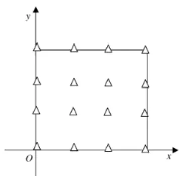
colloca-tion points. Here, the collocacolloca-tion points are typically distributed in the interior domain as well as on the bound-ary (Fig. 1). After applying Eq. (9) in N collocation points and the following augmented conditions, the

unknown aj’s and the b’s can be solved (Madych, 1992).

aj

Σ

j = 1 N = 0 ajxj

Σ

j = 1 N = 0 ajyj

Σ

j = 1 N = 0 for 2D aj

Σ

j = 1 N = 0 ajxj

Σ

j = 1 N = 0 ajyj

Σ

j = 1 N = 0 ajzj

Σ

j = 1 N = 0 for 3D (10) Fig. 1 Collocation points for the dual reciprocity method

Therefore, the particular solution Φp(x) can be determined (Golberg and Chen, 1998):

Φp(x) = aj ri2j( – 2rij2+ 4rij2Ln[rij]) 6144

Σ

j = 1 N + b1x 3 6 + b2 y3 6 + b3 x2_{+ y}2 4 for 2D aj rij3 12

Σ

j = 1 N + b1x 3 6 + b2 y3 6 + b3z 3 6 + b4 x2_{+ y}2_{+ z}2 6 for 3D (11) With the substitution of the Eq. (1) into the modified initial and boundary conditions of the ho-mogeneous Eq. (8), the result will be a well-posed homogeneous equation. The MFS is then applied to solve the equation. Since the diffusion fundamental s o l u t i o n s a t i s f i e s t h e h o m o g e n e o u s d i f f u s i o n equation, the solution can be assumed to be a linear combination of the fundamental solution of the dif-fusion operator. Therefore, the numerical solutions of the diffusion equation will be of the following form

Φh(x, t) =

Σ

cjG(x, t;ξj,τj) j = 1

N i + Nb

(12) where x represents the location of the field points and

ξj gives the location of the source points. Moreover,

t and τj are the time of the field and source points

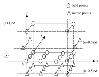
respectively, Ni and Nb are the number of initial and boundary source points and cj’s are the undetermined coefficients, which can be determined by the method of collocation. The distributions of the field points and the source points are illustrated in Fig. 2 for a 2D situation. In Fig. 2, the field points are placed at the boundary portion at t=(n+1)∆t and at the interior do-main at t=n∆t. The source points are placed in the same position but at different time levels. By collo-cating these field points and using Eq. (8), a linear matrix system with dimension Ni+Nb can be formed as follows: Aij{cj}={di} (13) where Aij= e– xi–ξj 2 4k(t_i–τ_j) – x_i–ξ_j24k(t_i–τ_j) (4πk ti–τj) m/2 for ti>τj 0 for ti≤τj

The vector {di} is the combination of initial and boundary conditions. After inverting the matrix system, the coefficients {cj} can be obtained, and then the homogenous solution at t=(n+1)∆t can be acquired from Eq. (12).

If the homogeneous solution Φh(x, t) and the par-ticular solution Φp(x) are solved, the solution Φ(x, t) of the original diffusion equation is obtained by us-ing the superposition principle of Eq. (6). Therefore, the procedure can be repeated until either the termi-nal time or a steady state solution is achieved.

IV. RESULTS AND DISCUSSIONS

The proposed numerical scheme, the MFS-DRM model based on the diffusion fundamental solution, is validated by comparing the results obtained with the analytical solutions for diffusion problems with Dirichlet boundary conditions. Moreover, compari-sons with the MFS-DRM model based on the modi-fied Helmholtz fundamental solution are also carried out. The effectiveness of the method is verified by solving 2D and 3D nonhomogeneous diffusion prob-lems and the results obtained are discussed in the fol-lowing sections. The collocation points of the 2D DRM for the particular solutions are shown in Fig. 1. On the other hand, the source points and the field points of the MFS based on the diffusion fundamen-tal solution are depicted in Fig. 2 for a 2D problem, and the points for the 2D MFS based on the modified Helmholtz fundamental solution are described in Fig. 3.

1. 2D Diffusion Problem

The proposed method is utilized to study two examples of 2D diffusion problems in a square slab of size [0,1]×[0,1].

Fig. 2 Schematic diagram of source and field points for the MFS based on diffusion fundamental solution

Example 1: G.E.:∂_∂u t =∇ 2 u –6x + 6y + 2 12 I.C.: u(x, y, t=0)

=2(cos[πx]+sin[πy])+x

3_{+ y}3_{+ x}2_{+ y}

12

B.C.:

u(0, y, t) = 2(1 + sin[πy])e–π2_t

+y

3_{+ y}

12

u(1, y, t) = 2(– 1 + sin[πy])e–π2_t

+y

3_{+ y + 2}

12

u(x, 0, t) = 2cos[πx]e–π2_t

+x3₁₂+ x2

u(x, 1, t) = 2cos[πx]e–π2_t

+x3+ x2+ 2 12

(14) The analytical solution of the problem is given by u(x, y, t)

=2(cos[πx]+sin[πy])e−π2t₊x3+ y3+ x2+ y

12 (15)

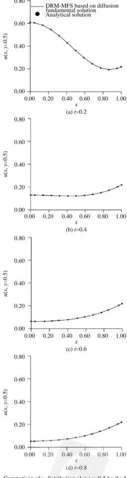
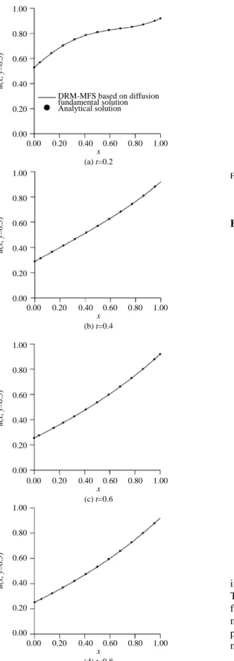
The comparison between the MFS-DRM model, based on the diffusion fundamental solution, and the analytical solution of the u-distribution along y=0.5 is depicted in Fig. 4. The results show generally good agreement, with the analytical solution in different time stages. In the figure, the gradient between the end surfaces decreases as time increases, thus ap-proaching a steady state condition. The variations clearly demonstrate the physics underlying the diffu-sion process. Moreover, Fig. 5 and Fig. 6 show the time evolution history at (0.5, 0.5) of the solution and the absolute error, respectively, for the MFS-DRM model based on the diffusion fundamental solution, and for the MFS-DRM model based on the modified Fig. 3 Schematic diagram of source and field points for the MFS

based on modified Helmholtz fundamental solution

Fig. 4 Comparison of u-distribution along y=0.5 by the MFS-DRM model based on diffusion fundamental solution (a) t=0.2; (b) t=0.4; (c) t=0.6; (d) t=0.8 (Nodes: 11×11, dt=0.07) 0.80 0.60 0.40 0.20 0.00 0.00 0.20 0.40 0.60 0.80 1.00 DRM-MFS based on diffusion fundamental solution Analytical solution x (a) t=0.2 u (x , y=0.5) 0.80 0.60 0.40 0.20 0.00 0.00 0.20 0.40 0.60 0.80 1.00 x (b) t=0.4 u (x , y=0.5) 0.80 0.60 0.40 0.20 0.00 0.00 0.20 0.40 0.60 0.80 1.00 x (c) t=0.6 u (x , y=0.5) 0.80 0.60 0.40 0.20 0.00 0.00 0.20 0.40 0.60 0.80 1.00 x (d) t=0.8 u (x , y=0.5)

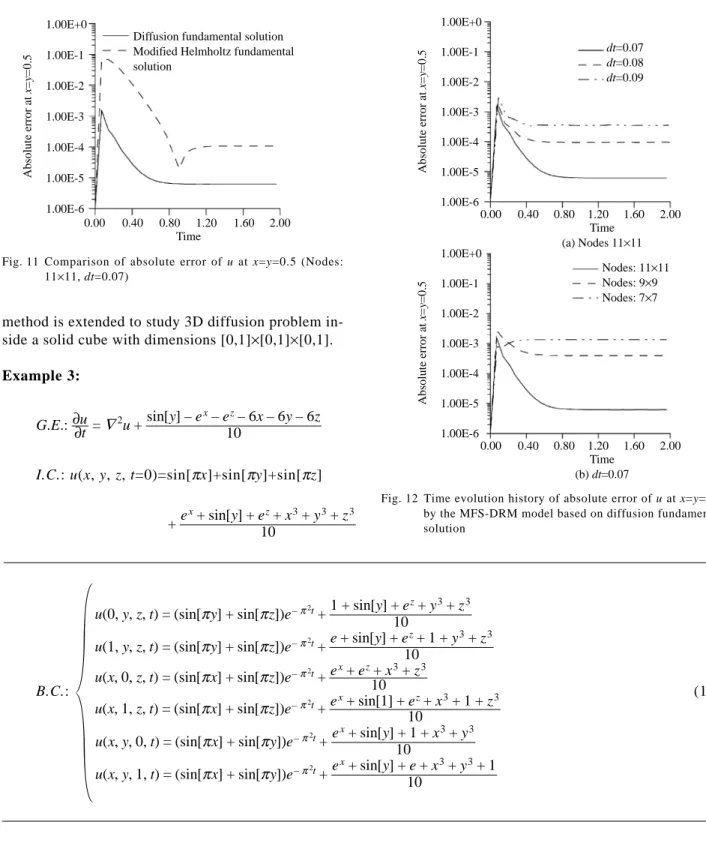
Helmholtz fundamental solution. In Fig. 6, the MFS-DRM model based on the diffusion fundamental so-lution shows better performance than the MFS-DRM model based on the modified Helmholtz fundamental solution, since the diffusion fundamental solution is a time-dependent function, which is capable of

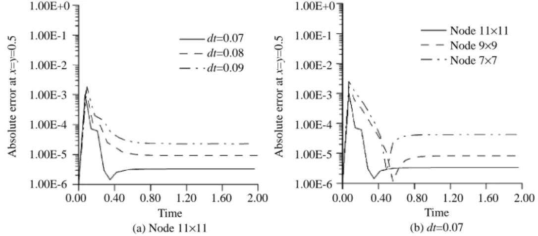
cap-turing the transient process much better (two order accuracy). On the other hand, Fig. 7 and Fig. 8 de-pict the error histograms for the two methods for dif-f e r e n t n u m b e r s o dif-f p o i n t s a n d d i dif-f dif-f e r e n t t i m e increments, in which more points and smaller time increments generally give better results, as expected. Fig. 5 Comparison of time evolution of u at x=y=0.5 (Nodes:

11×11, dt=0.07)

Fig. 6 Comparison of absolute error of u at x=y=0.5 (Nodes: 11×11, dt=0.07) 2.50 2.00 1.50 1.00 0.50 0.00 0.00 0.40 0.80 1.20 Time 1.60 2.00 u (0.5, 0.5) Analytical solution

Diffusion fundamental solution Modified Helmholtz fundamental solution 1.00E+0 1.00E-1 1.00E-2 1.00E-3 1.00E-4 1.00E-5 1.00E-6

Diffusion dundamental solution Modified Helmholtz fundamental solution 0.00 0.40 0.80 1.20 Time Absolute error at x= y=0.5 1.60 2.00

Fig. 7 Time evolution history of absolute error of u at x=y=0.5 by the MFS-DRM model based on diffusion fundamental solution 1.00E+0 1.00E-1 1.00E-2 1.00E-3 1.00E-4 1.00E-5 1.00E-6 dt=0.07 dt=0.08 dt=0.09 0.00 0.40 0.80 1.20 Absolute error at x= y=0.5 1.60 2.00 1.00E+0 1.00E-1 1.00E-2 1.00E-3 1.00E-4 1.00E-5 1.00E-6 Node 11×11 Node 9×9 Node 7×7 0.00 0.40 0.80 1.20 Absolute error at x= y=0.5 1.60 2.00 Time (a) Node 11×11 Time (b) dt=0.07

Fig. 8 Time evolution history of absolute error of u at x=y=0.5 by the MFS-DRM model based on modified Helmholtz fundamental solution 1.00E+0 1.00E-1 1.00E-2 1.00E-3 1.00E-4 1.00E-5 1.00E-6 dt=0.07 dt=0.08 dt=0.09 0.00 0.40 0.80 1.20 Absolute error at x= y=0.5 1.60 2.00 1.00E+0 1.00E-1 1.00E-2 1.00E-3 1.00E-4 1.00E-5 1.00E-6 Node 11×11 Node 9×9 Node 7×7 0.00 0.40 0.80 1.20 Absolute error at x= y=0.5 1.60 2.00 Time (a) Node 11×11 Time (b) dt=0.07

Fig. 9 Comparison of u-distribution along y=0.5 by the MFS-DRM model based on diffusion fundamental solution (a) t=0.2; (b) t=0.4; (c) t=0.6; (d) t=0.8 (Nodes: 11×11, dt=0.07) 1.00 0.80 0.60 0.40 0.20 0.00 0.00 0.20 0.40 0.60 0.80 1.00 DRM-MFS based on diffusion fundamental solution Analytical solution x (a) t=0.2 u (x , y=0.5) 1.00 0.80 0.60 0.40 0.20 0.00 0.00 0.20 0.40 0.60 0.80 1.00 x (b) t=0.4 u (x , y=0.5) 1.00 0.80 0.60 0.40 0.20 0.00 0.00 0.20 0.40 0.60 0.80 1.00 x (c) t=0.6 u (x , y=0.5) 1.00 0.80 0.60 0.40 0.20 0.00 0.00 0.20 0.40 0.60 0.80 1.00 x (d) t=0.8 u (x , y=0.5)

Fig. 10 Comparison of time evolution of u at x=y=0.5 (Nodes: 11×11, dt=0.07) 3.00 2.00 1.00 0.00 0.00 0.40 0.80 1.20 Time u (0.5, 0.5) 1.60 2.00 Analytical solution

Diffusion fundamental solution Modified Helmholtz fundamental solution Example 2: G.E.:∂_∂u_t =∇2u –ye x_{– x sin[y]} 2

I.C.: u(x, y, t=0)=cos[πx]+cos[πy]+sin[πx]

+sin[πy]+ye

x_{+ x sin[y]} 2

B.C.:

u(0, y, t) = (1 + cos[πy] + sin[πy])e–π2_t

+ y 2

u(1, y, t) = (– 1 + cos[πy] + sin[πy])e–π2_t

+ ye + sin[y]

2

u(x, 0, t) = (cos[πx] + 1 + sin[πx])e–π2_t

u(x, 1, t) = (cos[πx] – 1 + sin[πx])e–π2_t

+ex+ x sin[1] 2

(16) The analytical solution of the problem is given by

u(x, y, t)=(cos[πx]+cos[πy]+sin[πx]

+sin[πy])e−π2t

+ye

x_{+ x sin[y]}

2 (17)

The numerical results of this example are shown in Figs. 9-13. They are similar to the previous example. The results of the MFS-DRM model based on the dif-fusion fundamental solution also show very good agree-ment with the analytical solution and demonstrate better performance than the MFS-DRM model based on the modified Helmholtz fundamental solution.

2. 3D Diffusion Problem

method is extended to study 3D diffusion problem in-side a solid cube with dimensions [0,1]×[0,1]×[0,1].

Example 3:

G.E.:∂_∂u_t =∇2u +sin[y] – e

x_{– e}z_{– 6x – 6y – 6z} 10

I.C.: u(x, y, z, t=0)=sin[πx]+sin[πy]+sin[πz]

+e

x_{+ sin[y] + e}z_{+ x}3_{+ y}3_{+ z}3

10

Fig. 12 Time evolution history of absolute error of u at x=y=0.5 by the MFS-DRM model based on diffusion fundamental solution 1.00E+0 1.00E-1 1.00E-2 1.00E-3 1.00E-4 1.00E-5 1.00E-6 dt=0.07 dt=0.08 dt=0.09 0.00 0.40 0.80 1.20 Time (a) Nodes 11×11 Absolute error at x= y=0.5 1.60 2.00 1.00E+0 1.00E-1 1.00E-2 1.00E-3 1.00E-4 1.00E-5 1.00E-6 0.00 0.40 0.80 1.20 Time (b) dt=0.07 Absolute error at x= y=0.5 1.60 2.00 Nodes: 11×11 Nodes: 9×9 Nodes: 7×7 Fig. 11 Comparison of absolute error of u at x=y=0.5 (Nodes:

11×11, dt=0.07) 1.00E+0 1.00E-1 1.00E-2 1.00E-3 1.00E-4 1.00E-5 1.00E-6

Diffusion fundamental solution Modified Helmholtz fundamental solution 0.00 0.40 0.80 1.20 Time Absolute error at x= y=0.5 1.60 2.00 B.C.:

u(0, y, z, t) = (sin[πy] + sin[πz])e–π2_t

+1 + sin[y] + e

z_{+ y}3_{+ z}3

10

u(1, y, z, t) = (sin[πy] + sin[πz])e–π2_t

+e + sin[y] + e

z_{+ 1 + y}3_{+ z}3

10

u(x, 0, z, t) = (sin[πx] + sin[πz])e–π2_t

+ex+ ez+ x3+ z3 10

u(x, 1, z, t) = (sin[πx] + sin[πz])e–π2_t

+e

x_{+ sin[1] + e}z_{+ x}3_{+ 1 + z}3

10

u(x, y, 0, t) = (sin[πx] + sin[πy])e–π2_t

+e

x_{+ sin[y] + 1 + x}3_{+ y}3

10

u(x, y, 1, t) = (sin[πx] + sin[πy])e–π2_t

+e

x_{+ sin[y] + e + x}3_{+ y}3_{+ 1}

10

(18)

The analytical solution of the problem is given by

u(x, y, z, t)=(sin[πx]+sin[πy]+sin[πz])e−π2t

+e

x_{+ sin[y] + e}z_{+ x}3_{+ y}3_{+ z}3

10 (19)

Figure 14 shows the time evolution history at (0.5. 0.5, 0.5) of the solution for the MFS-DRM model

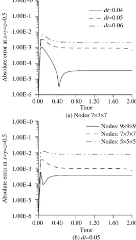
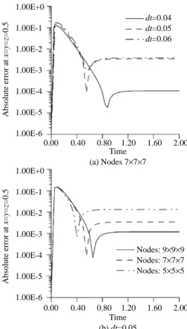
based on the diffusion fundamental solution as well as the MFS-DRM model based on the modified Helmholtz fundamental solution. On the other hand, Fig. 15 shows the time evolution history of the abso-lute error for the two methods, in which the MFS-DRM model based on the diffusion fundamental solution, which has better performance. Finally, Fig. 16 and Fig. 17 depict the error histograms for the two methods for different numbers of points and

different time increments, in which more points and smaller time increments in general will give better results, as before.

V. CONCLUSIONS

Transient diffusion problems with time-indepen-dent source terms in multi-dimensions are solved Fig. 13 Time evolution history of absolute error of u at x=y=0.5 by the MFS-DRM model based on modified Helmholtz fun-damental solution 1.00E+0 1.00E-1 1.00E-2 1.00E-3 1.00E-4 1.00E-5 1.00E-6 dt=0.07 dt=0.08 dt=0.09 0.00 0.40 0.80 1.20 Time (a) Nodes 11×11 Absolute error at x= y=0.5 1.60 2.00 1.00E+0 1.00E-1 1.00E-2 1.00E-3 1.00E-4 1.00E-5 1.00E-6 0.00 0.40 0.80 1.20 Time (b) dt=0.07 Absolute error at x= y=0.5 1.60 2.00 Nodes: 11×11 Nodes: 9×9 Nodes: 7×7

Fig. 14 Comparison of time evolution of u at x=y=z=0.5 (Nodes: 7×7×7, dt=0.04) 4.00 3.00 2.00 1.00 0.00 0.00 0.40 0.80 1.20 Time u (0.5, 0.5, 0.5) 1.60 2.00 Analytical solution

Diffusion fundamental solution

Modified Helmholtz fundamental solution

Fig. 15 Comparison of time evolution of absolute error of u at x=y=z=0.5 (Nodes: 7×7×7, dt=0.04) 1.00E+0 1.00E-1 1.00E-2 1.00E-3 1.00E-4 1.00E-5 1.00E-6

Diffusion fundamental solution Modified Helmholtz fundamenal solution 0.00 0.40 0.80 1.20 Time Absolute error at x= y= z=0.5 1.60 2.00

Fig. 16 Time evolution history of absolute error of u at x=y=z=0.5 by the MFS-DRM model based on diffusion fundamental solution 1.00E+0 1.00E-1 1.00E-2 1.00E-3 1.00E-4 1.00E-5 1.00E-6 dt=0.04 dt=0.05 dt=0.06 0.00 0.40 0.80 1.20 Time (a) Nodes 7×7×7 Absolute error at x= y= z=0.5 1.60 2.00 1.00E+0 1.00E-1 1.00E-2 1.00E-3 1.00E-4 1.00E-5 1.00E-6 0.00 0.40 0.80 1.20 Time (b) dt=0.05 Absolute error at x= y= z=0.5 1.60 2.00 Nodes: 9×9×9 Nodes: 7×7×7 Nodes: 5×5×5

using the MFS-DRM model based on the direct us-age of the diffusion fundamental solution. The MFS is adopted to obtain the homogeneous solution and the DRM is utilized to solve the nonhomogeneous source term. The generally adopted Laplace trans-form and finite difference scheme for the time derivative term are not required in the proposed nu-merical solution procedure. The independent time

variable was treated as one of the solution domains in the time-dependent fundamental solutions and this space-time unification makes it possible to make use of the MFS to obtain the numerical solutions of the homogeneous diffusion equation without transforma-tion or difference discretizatransforma-tion for the time domain. By properly locating the source points and the field points at every time level, the solutions were advanced in time until the system reached steady state conditions. The numerical procedure developed in the present work was validated by comparing its re-sults with the rere-sults obtained by analytical solutions as well as the traditional MFS-DRM model based on the modified Helmholtz fundamental solution for 2D and 3D diffusion problems under the Dirichlet bound-ary conditions. The excellent agreement with the ana-lytical results and better performance than the tradi-tional method indicate the effectiveness of the present method to solve diffusion equations with time-inde-pendent source terms without requiring any time transformation or time discretization. Besides, the unification of time and space variables makes the re-moval of singularities with respect to both space and time except t−τ=0 possible.

ACKNOWLEDGMENTS

The National Science Council of Taiwan is gratefully acknowledged for providing financial sup-port of NSC 92-2611-E-002-007 to carry out the present work.

REFERENCES

Atluri, S. N., and Zhu, T., 1998, “A New Meshless Local Petrov-Galerkin (MLPG) Approach in Computational Mechanics,” Computational Mechanics, Vol. 22, No. 2, pp. 117-127.

Balakrishnan, K., and Ramachandran, P. A., 2000, “The Method of Fundamental Solutions for Lin-ear Diffusion-Reaction Equations,” Mathemati-cal and Computer Modeling, Vol. 31, Nos. 2-3, pp. 221-237.

Berger, J. R., and Karageorghis, A., 1999, “The Method of Fundamental Solutions for Heat Con-duction in Layered Materials,” International Journal for Numerical Methods in Engineering, Vol. 45, No. 11, pp. 1681-1694.

Bialecki, R. A., Jurgas, P., and Kuhn, G., 2002, “Dual Reciprocity BEM without Matrix Inversion for Transient Heat Conduction,” Engineering Analy-sis with Boundary Elements, Vol. 26, No. 3, pp. 227-236.

Bulgakov, V., Sarler, B., and Kuhn, G., 1998, “Itera-tive Solution of Systems of Equations in the Dual Reciprocity Boundary Element Method for the Diffusion Equation,” International Journal for Numerical Methods in Engineering, Vol. 43, No. 4, pp. 713-732.

Chawla, M. M., and Al-Zanaidi, M. A., 1999, “An Extended Trapezoidal Formula for the Diffusion Equation,” Computers and Mathematics with Applications, Vol. 38, pp. 51-59.

Chen, C. S., Golberg, M. A., and Hon, Y. C., 1998a, “The Method of Fundamental Solutions and Q u a s i - M o n t e - C a r l o M e t h o d f o r D i f f u s i o n Equations,” International Journal for Numerical Methods in Engineering, Vol. 43, No. 8, pp. 1421-1435.

Chen, C. S., Golberg, M. A., and Rashed, Y. F., 1998b, “A Mesh Free Method for Linear Diffu-sion Equations,” Numerical Heat Transfer Part B, Vol. 33, pp. 469-486.

Chen, J. T., Hong, H.-K., Yeh, C. S., and Chyuan, S. W.,1996, “Integral Representations and Regu-larizations for a Divergent Series Solution of a Beam Subjected to Support Motions,” Earthquake Engineering and Structural Dynamics, Vol. 25, pp. 909-925.

Golberg, M. A., 1995, “The Method of Fundamental Solutions for Poisson’s Equation,” Engineering Fig. 17 Time evolution history of absolute error of u at x=y=z=0.5

by the DRM-MFS based on modified Helmholtz funda-mental solution 1.00E+0 1.00E-1 1.00E-2 1.00E-3 1.00E-4 1.00E-5 1.00E-6 dt=0.04 dt=0.05 dt=0.06 0.00 0.40 0.80 1.20 Time (a) Nodes 7×7×7 Absolute error at x= y= z=0.5 1.60 2.00 1.00E+0 1.00E-1 1.00E-2 1.00E-3 1.00E-4 1.00E-5 1.00E-6 0.00 0.40 0.80 1.20 Time (b) dt=0.05 Absolute error at x= y= z=0.5 1.60 2.00 Nodes: 9×9×9 Nodes: 7×7×7 Nodes: 5×5×5

Analysis with Boundary Elements, Vol. 16, No. 3, pp. 205-213.

Golberg, M. A., and Chen, C. S., 1998, “The Method o f F u n d a m e n t a l S o l u t i o n s f o r P o t e n t i a l , Helmholtz and Diffusion Problems,” Boundary Integral Methods, Computational Mechanics Publications, Boston, U.S.A., pp. 103-176. Hobson, J. M., Wood, N., and Mason, P. J., 1996, “A

New Finite-Difference Diffusion Scheme,” Jour-nal of ComputatioJour-nal Physics, Vol. 125, No. 1, pp. 16-25.

Jones, W. P., and Menzies, K. R., 2000, “Analysis of the Cell-Centered Finite Volume Method for the Diffusion Equation,” Journal of Computational Physics, Vol. 165, No. 1, pp. 45-68.

Kansa, E. J., 1990a, “Multiquadrics - a Scattered Data Approximation Scheme with Applications to Computational Fluid Dynamics-I, Surface Ap-proximations and Partial Derivative Estimates,” Computers and Mathematics with Applications, Vol. 19, Nos. 8-9, pp. 127-145.

Kansa, E. J., 1990b, “Multiquadrics - a Scattered Data Approximation Scheme with Applications to Computational Fluid Dynamics II, Solutions to Parabolic, Hyperbolic and Elliptic Partial Differ-ential Equations,” Computers and Mathematics with Applications, Vol. 19, Nos. 8-9, pp. 147-161. Kim, H. G., and Atluri, S. N., 2000, “Arbitrary Place-ment of Secondary Nodes, and Error Control, in the Meshless Local Petrov-Galerkin (MLPG) Method,” Computer Modeling in Engineering and Sciences, Vol. 1, No. 3, pp. 11-32.

Lin, H., and Atluri, S. N., 2000, “Meshless Local Petrov-Galerkin (MLPG) Method for Convection-Diffusion Problems,” Computer Modeling in En-gineering and Sciences, Vol. 1, No. 2, pp. 45-60. Lin, H., and Atluri, S. N., 2001, “The Meshless Local Petrov-Galerkin (MLPG) Method for Solv-ing Incompressible Navier-Stokes Equations,” Computer Modeling in Engineering and Sciences, Vol. 2, No. 2, pp. 117-142.

Madych, W., 1992, “Miscellaneous Error Bounds for Multiquadric and Related Interpolants,” Comput-ers and Mathematics with Applications, Vol. 24, pp. 121-138.

Nardini, D., and Brebbia, C. A., 1982, “A New Ap-proach to Free Vibration Analysis Using Bound-ary Elements,” BoundBound-ary Element Methods in Engineering, Springer-Verlag, Berlin, German. Oden, J. T., Babuska, I., and Baumann, C. E., 1998,

“A Discontinuous hp Finite Element Method for Diffusion Problems,” Journal of Computational Physics, Vol. 146, No. 2, pp. 491-519.

Poullikkas, A., Karageorghis, A., and Georgiou, G., 1998a, “Methods of Fundamental Solutions for Harmonic and Biharmonic Boundary Value

Problems,” Computational Mechanics, Vol. 21, Nos. 4-5, pp. 416-423.

Poullikkas, A., Karageorghis, A., and Georgiou, G., 1998b, “The Method of Fundamental Solutions for Inhomogeneous Elliptic Problems,” Compu-tational Mechanics, Vol. 22, No. 1, pp. 100-107. Ramachandran, P. A., 2002, “Method of Fundamen-tal Solutions: Singular Value Decomposition Analysis,” Communications in Numerical Meth-ods in Engineering, Vol. 18, pp. 789-801. Smyrlis, Y. S., Karageorghis, A., and Georgiou, G.,

2001, “Some Aspects of the One-Dimensional Ver-sion of the Method of Fundamental Solutions,” Computers and Mathematics with Applications, Vol. 41, pp. 647-657.

Sutradhar, A., Paulino, G. H., and Gray, L. J., 2002, “Transient Heat Conduction in Homogeneous and Non-Homogeneous Materials by the Laplace Transform Galerkin Boundary Element Me-thod,” Engineering Analysis with Boundary Ele-ments, Vol. 26, No. 3, pp. 119-132.

Teixeira, J., 1999, “Stable Schemes for Partial Dif-ferential Equations: the One-Dimensional Diffu-sion Equation,” Journal of Computational Physics, Vol. 153, No. 2, pp. 403-417.

Wordelman, C. J., Atluri, S. N., and Ravaioli, U., 2000, “A Meshless Method for the Numerical So-lution of the 2D and 3D Semiconductor Poisson Equation,” Computer Modeling in Engineering and Sciences, Vol. 1, No. 1, pp. 121-126. Zerroukat, M., 1999, “A Boundary Element Scheme

f o r D i f f u s i o n P r o b l e m s U s i n g C o m p a c t l y Supported Radial Basis Functions,” Engineering Analysis with Boundary Elements, Vol. 23, No. 3, pp. 201-209.

Zhu, S. P., 1998, “Solving Transient Diffusion Pro-blems: Time-Dependent Fundamental Solution Approaches Versus LTDRM Approaches,” Engi-neering Analysis with Boundary Elements, Vol. 21, No. 1, pp. 87-90.

Zhu, S. P., Liu, H. W., and Lu, X. P., 1998, “A Com-bination of LTDRM and ATPS in Solving Diffu-sion Problems,” Engineering Analysis with Bound-ary Elements, Vol. 21, No. 3, pp. 285-289. Zhu, T., Zhang, J., and Atluri, S. N., 1998, “A Meshless

Local Boundary Integral Equation (LBIE) Method for Solving Nonlinear Problems,” Computational Mechanics, Vol. 22, No. 2, pp. 174-176.

Manuscript Received: Dec. 12, 2003 Revision Received: Apr. 25, 2004 and Accepted: May 07, 2004

APPENDIX

the modified Helmholtz fundamental solution (Chen et al., 1998b; Golberg and Chen, 1998). First of all, we apply the finite difference in time to the diffusion Eq. (1). That is ∂Φ(x, t) ∂t _{t = n∆t}= Φ(n + 1) (x) –Φ(n)(x) ∆t (A1)

where ∆t is an a priori constant of the time step, and

Φ(n)

(x) is defined as Φ(x, n∆t). Applying the defini-tion (A1) to the diffusion Eq. (1), we are capable of obtaining Φ(n + 1) (x) –Φ(n)(x) ∆t = k∇ 2_Φ(n + 1) (x) + A(x) in Ω (A2) or ∇2Φ(n+1) (x)−λ2Φ(n+1) (x)=−λ2Φ(n) (x)−A(x) k in Ω (A3) where λ2₌ 1

∆tk. Combining with the boundary condi-tion (3) and the initial condicondi-tion (2), this will result in Φ(0) (x)=B(x) in Ω Φ(n+1) (x)=C(n+1) (x) on Γ1 ∂Φ(n + 1) ∂n (x)=D (n+1) (x) on Γ2 (A4) The Eq. (A3) and Eq. (A4) can be viewed as a series of modified Helmholtz equations for the unknown se-ries of functions, Φ(1) (x), Φ(2) (x), Φ(3) (x), with known initial function Φ(0) (x)=B(x).

In order to apply the MFS-DRM model based on the modified Helmholtz fundamental solution to solve the equation, we first decompose the unknown function to Φ(n + 1) (x) =Φh (n + 1) (x) +Φp (n + 1) (x) (A5)

where the particular solution, Φp (n + 1) (x), satisfies ∇2_Φ p (n + 1) (x) –λ2Φp (n + 1) (x) = –λ2Φ(n)(x) –A(x) k in Ω (A6)

and the homogeneous solution, Φh (n + 1) (x), satisfies ∇2_Φ h (n + 1)_{(x) –λ}2_Φ h (n + 1)_{(x) = 0} in Ω Φh (n + 1)_{(x) = C}(n + 1)_{(x) –Φ} p (n + 1)_(x) in Γ1 ∂Φh (n + 1) ∂n (x) = D (n + 1) (x) –∂Φp (n + 1) ∂n (x) in Γ 2 (A7) The particular solution corresponding to Eq. (A6) can be approximated by the DRM for the source

term −λ2Φ(n) (x)−A(x) k –λ2Φ(n)(x) –A(x) k = ajrij2Ln[rij] + b1x + b2y + b3

Σ

j = 1 N for 2D ajrij+ b1x + b2y + b3z + b4

Σ

j = 1 N for 3D (A8)

in which the details are the same as the DRM for the diffusion equation posted before. Therefore, the par-ticular solution Φp

(n + 1)

(x) can be determined (Golberg and Chen, 1998): Φp (n + 1) (x) = aj

Σ

j = 1 N {– 4 λ4(K0(λrij) + Ln[rij]) –rij 2_Ln[r ij] λ2 } – 4_λ4 – b1x λ2 – b2y λ2 – b3 λ2 for 2D aj

Σ

j = 1 N { 2 λ4 rij (e–λrij – 1) – rij λ2} –b1x λ2 – b2y λ2 – b3z λ2 – b4 λ2 for 3D (A9) where K0(•) is the zero order modified Bessel

function of the second kind.

With the substitution of the Eq. (A9) into the governing equation of the homogeneous Eq. (A7), the result will be a well-posed homogeneous modified Helmholtz equation, and hence it is capable of being solved. Since the modified Helmholtz fundamental solution satisfies the modified Helmholtz equation, we may assume the homogeneous solution is a linear combination of the fundamental solution of the modi-fied Helmholtz operator, i.e.:

Φh (n + 1) (x) =

Σ

cig( x –ξi ) i = 1 N (A10) where

g(r) = 1 2πK0[λr] for 2D e–λr 4πr for 3D (A11)

is the fundamental solution of the modified Helmholtz operator (Chen et al., 1998b; Golberg and Chen, 1998), x represents the location of the field points, ξi gives the location of the source points, r=|x−ξi| is the distance, and N is the number of source points and field points. The source points are typically distrib-uted away from the boundary field points to avoid the singularity as shown in Fig. 3. By collocating these field points and using Eq. (A7), a linear matrix system can be formed as follows

Aij{cj}={di} (A12) where Aij = 1 2πK0[λ xi–ξj] for 2D e–λxi–ξj 4π xi–ξj for 3D

The vector {di} stems from the boundary conditions. After inverting the matrix system, the coefficients {cj} can be obtained, and then the ho-mogenous solution at t=(n+1)∆t can be acquired.

After the homogenous solution and the particu-lar solution are solved, the solution of the original diffusion equation at t=(n+1)∆t can be obtained by the superposition principle of Eq. (A5). Therefore, the procedure can be repeated until either the termi-nal time or a steady state solution is achieved.