國立高雄大學資訊工程學系(研究所)
士論文
以投資者情緒指標為基礎的多樣群組股票組合最佳化之研
究
A Study on Diverse Group Stock Portfolio
Optimization Based on Investor Sentiment Index
研究生:朱世祺 撰
指導教授:洪宗貝 博士
指導教授:陳俊豪 博士
致謝
在這兩年的碩士生涯中,無論是學校的課程或是實驗室的訓練都使我受益良多。如 今在許多人的幫助下順利完成了本篇碩士論文。 首先非常感謝指導我的兩位教授洪宗貝老師以及陳俊豪老師。在實驗室裡,洪老師 總是會適時的給予我建議,點出我所需要注意的地方,除了在研究領域所給予的幫助外, 在表達的能力上提醒我所要加強的地方,進而提升我的思維邏輯、面對事情的態度及做 事情細膩度。陳老師在我的研究中幫助了我許多,就算工作繁忙,也會抽空與我進行遠 端會議,使我的專業領域知識可以有所提升,實作的方面也給予了許多實質的幫助,在 此致上由衷的謝意。 接著感謝我碩士論文的口試委員,藍國誠老師及蘇家輝老師。在百忙之中還抽空參 加我的口試會議,並對我的論文提出指教及需要修正的地方,給予了許多建設性及前瞻 性的建議,使我的碩士論文內容可以更加豐富。 此外也要感謝跟我一起奮鬥的夥伴們,在實驗室裡的明泰學長、菊添學長、偉銘學 長、宗達學長、昆毅學長、元慶學長、志峰學長,感激這陣子你們的照顧,冀正、盧宏、 雨棠、仁豪、宇喬、翔維、秉洋、永瀚、佳哲,感謝你們在實驗室幫忙實驗室的事務, 讓我可以更加專心的做研究。另外感謝政輔、侑廷、芝君、柏鈞、力中、耀皚、尚益、 厚傑、柏豪、昀達,有了你們的陪伴讓我的碩士生涯可以更加精采。 最後,要感謝我最重要的家人,無條件的支持我走完碩士這兩年,背後的付出我都 銘感於心,真心的感謝你們。 朱世祺 謹致 人工智慧實驗室 2017.9.14以投資者情緒指標為基礎的多樣群組股票組合最佳化之研
究
指導教授:洪宗貝 博士 國立高雄大學資訊工程所 共同指導教授:陳俊豪 博士 淡江大學資訊工程所 學生:朱世祺 國立高雄大學資訊工程所 摘要 金融資料分析一直都是既有趣且具有挑戰性的議題而投資組合最佳化也是其最熱 門的研究主題之一。過去數十年已有許多演算法被設計來解決投資組合最佳化問題,其 中部分研究用於尋找群組股票投資組合,將多個相似的股票群組在一起,從每個股票群 組挑選一股票合起來則可形成一個投資組合,故給定一個群組股票投資組合可產生許多 不同的投資組合。此外投資人情緒的研究也是金融資料分析的熱門主題,且一些學者指 出投資人情緒確實會影響股市的波動。因此,本研究旨在利用兩個投資人情緒指標於群 組遺傳演算法中以找出群組股票投資組合,除了提供不同的投資組合外,亦以可提供合 適的買賣時機。在資料前處理時,首先挑選出文獻中被建議的情緒指標因子以形成交易 策略,並產生個股的買賣訊號。然後根據之前的方法,每一可能的群組股票投資組合被 編改成三個部分表示,分別為群組、股票與投資組合。在評估函數部分,除了利用既有 的組合滿意度、群組平衡、價格平衡與數量平衡等考慮因素外,亦設計投資者情緒風險 因子一起進行染色體評估,藉以找出更好的群組股票投資組合。最後在實驗部分,我們 使用一組實際的股票資料來驗證並顯示所提方法的有效性與優點。 關鍵字:投資人情緒指標、交易策略、群組基因演算法、群組投資組合、最大多樣性群 組問題A Study on Diverse Group Stock Portfolio Optimization
Based on Investor Sentiment Index
Advisor: Dr. Tzung-Pei Hong
Institute of Computer Science and Information Engineering National University of Kaohsiung
Co-Advisor: Dr. Chun-Hao Chen
Institute of Computer Science and Information Engineering Tamkang University
Student: Shih-Chi Chu
Institute of Computer Science and Information Engineering National University of Kaohsiung
Abstract
Financial data analysis has always been an interesting and challenging issue and stock portfolio optimization is one of its most popular researchh topics. In the past decades, many algorithms have been designed to solve the stock portfolio optimization problem, with some of them used for obtaining a group stock portfolio which consists of a set of stock groups with similar stocks gathered together. Stocks can then be selected from stock groups to form a stock portfolio. Thus, lots of stock portfolios can be generated from a group stock portfolio. Besides, research on investor sentiment is also very popular in financial data analysis, and some scholars claim that it has impact on the stock market. Hence, in this thesis, we will use two investor sentiment indices in the grouping genetic algorithm to obtain a group stock portfolio which can not only provide good portfolios but also indicate appropriate buy/sell trading signals. In data preprocessing, we first select inventor sentiment factors suggested in literature for forming the trading strategies to generate trading signals. Then according to a previous approach, we encode each possible group stock portfolio as three parts: grouping, stock and stock portfolio. The adopted fitness function consists of not only existing factors, including portfolio satisfaction, group balance, price balance and unit balance, but also a new factor called risk of investor sentiment, to evaluate the chromosomes for finding appropriate group stock portfolios. At last, experiments were conducted on a real stock dataset to verify and show the effectiveness and advantages of the proposed approach.
Keywords: investor sentiment index, trading strategy, grouping genetic algorithms, group stock portfolio, maximally diverse grouping problem
Content
摘要………...……….….……i Abstract……….………...………..…ii List of Figures……….………....….…. vi List of Tables……….……..………....….…………vii CHAPTER 1 Introduction……….……….1 1.1 Stock Portfolio……….………...…1 1.2 Investor Sentiment……….………....3CHAPTER 2 Related Work and Background Knowledge……….……….5
2.1 The M-V Model………...………..………5
2.2 Grouping Genetic Algorithm and Grouping Problem………....….….…..6
2.3 Maximally Diverse Grouping Problem……….…………...…8
2.4 Proposed Method for Stock Portfolio……….….….……...9
2.5 Investor Sentiment Index……….…..…………..10
CHAPTER 3 Proposed Approach………..………...12
3.1 Data preprocessing… ……….………..………...13
3.2 Components of the Proposed Approach……….…….………...…..20
3.2.2 Initial Population………..….……...……...21
3.2.3 Fitness Functions………..…...23
3.2.4 Genetic Operation……….……….……...31
3.2.4.1 Crossover………..……...31
3.2.4.2 Mutation and Inversion………..……….….……...32
3.3 The Proposed Algorithm………....……...……….…….………….………34
3.4 An Example……….39
CHAPTER 4 Experimental Result……….…….………...49
4.1 Data Descriptions……….…………..……….49
4.2 Analysis of Diverse Group Stock Portfolio……….………..……..…52
4.3 Comparison of the Proposed Approach and Existing Approaches………....……..55
CHAPTER 5 Conclusion and Future Works……….………...….57
List of Figures
Fig. 1: The flowchart of the proposed approach………..…..…..………….….12
Fig. 2: The encoding scheme of chromosome……….………..….………...20
Fig. 3: An example of encoding scheme……….…….……..….…….………..…21
Fig. 4: The 46 stock price series……….……..….………...50
Fig. 5. The stock-price series in Group1 of the chromosome………..………..53
Fig. 6. The stock-price series in Group2 of the chromosome………..……….…53
Fig. 7. The stock-price series in Group3 of the chromosome………..………….……53
Fig. 8. The stock-price series in Group4 of the chromosome………..……….…54
Fig. 9. The stock-price series in Group5 of the chromosome………..………...54
Fig. 10. The stock-price series in Group6 of the chromosome………..………...54
List of Tables
Table 1: Six cases for the two investor sentiment indices.………….…...….………17Table 2: Cash dividend yields of two companies.……….………22
Table 3: The cash dividend yield (yi) of companies.……….….………...22
Table 4: Proportion of average cash dividend of each group.………23
Table 5: The price and trading signals.……….……….…25
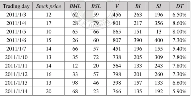
Table 7: Trading data on the stock from 2011/1/3 to 2011/1/14.……….………….39
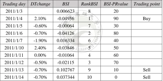
Table 8: The investor sentiment indices from 2011/1/3 to 2011/1/14.……….…….40
Table 9: The data of stocks used in this example.……….…………41
Table 10: The RIS of all chromosomes……….……….…44
Table 11: The portfolio satisfactions of all chromosomes...45
Table 12: The group balances of all chromosomes………..………….45
Table 13: The dissimilarity matrix of stocks………...46
Table 14: The diversity values of all chromosomes………..………….47
Table 15: The information of all stock categories in dataset………..…50
Table 16: The derived diverse GSPs with investor sentiment index………..…………52
CHAPTER 1
Introduction
1.1 Stock Portfolio
Since there were financial transactions in human economic activities, financial data analysis has been an issue of focus. Investors always hope that they can get a higher return for their money by using the results of financial information analysis to invest. In 1952, the theory of portfolio proposed by Markowitz laid the foundation for current investment. He used the stock's expected earnings and risk to construct the model called the mean-variance (M-V) model for acquiring a stock portfolio. After investors set the acceptable value of risk (VaR) by their needs, the model will be able to suggest to investors a portfolio of investment stocks with the greatest return on investment (ROI) under the limit of maximum VaR. Because different expected VaRs and ROIs will result in various portfolios, optimization techniques have been proposed for deriving appropriate portfolios based on the model.
However, providing only a stock portfolio to investors is not practical for real applications. For instance, there is a stock portfolio {s1: 2, s2: 5, s3: 3}. The stock portfolio means that it
suggests investors buy the stock s1 with the three purchased units, buy the stock s2 with the five
purchased units, and buy the stock s3 with the three purchased units. In this case, investors may
face a situation in which not all suggested stocks are suitable for their plans. For example, the stock price of s2 may be too high to buy. When this situation occurs, the situation will be much
better if other substitute stocks or stock portfolios could be suggested. Hence, the problem is shifted from finding a stock portfolio to mining a set of stock portfolios.
(GSP) [8]. In the approach, they use grouping genetic algorithm (GGA) to divide n stocks into K groups and make that the stocks in the same group are similar. Then they advise investors on GSP, which represents a set of stock portfolios, not a stock portfolio. For instance, assuming there are six stocks, they advise investors to buy the GSP as follows: G1: {s1, s2: 2}, G2: {s3, s4:
5}, G3: {s5, s6: 3}. This GSP represents dividing six stocks into three groups and suggests
investors buy the stock s1 or s2 with the two purchased units, buy the stock s3 or s4 with the five
purchased units, and buy the stock s5 or s6 with the three purchased units. It overcomes the
above-mentioned problem. If investors have no intention to choose s2, they can select s1 which
is similar to s2 to replace it. However, there is a problem that needs to be solved because the
above-mentioned approach does not take group diversity into consideration. For instance, assuming there are six stocks, stock symbols are s1, s2, s3, s4, s5, s6. The first two stocks belong
to the automobile. The last two stocks belong to the semiconductor. The middle two stocks belong to other electronics. If a negative news about the automotive industry was reported, then the advised GSP is still as follows: G1: {s1, s2: 2}, G2: {s3, s4: 5}, G3: {s5, s6: 3}. In this case,
investors have a high probability of not trying to hold any stocks that belong to the automobile. However, investors have no other option to replace s1 and s2 because all stocks in G1 belong to
the automobile.
To help investors out of this trouble, Chen et al. proposed an improved algorithm for mining group stock portfolio (GSP) called mining diverse group stock portfolio (DGSP) [9]. They take stock diversity into consideration. The approach makes every group in the advised GSP go for the highest diversity. After using this algorithm, the advised GSP may be followed:
G1: {s1, s3: 2}, G2: {s2, s5: 5}, G3: {s3, s6: 3}. It is found that the stocks’ industrial category in
the same group is different. This result represents that investors can choose another stock within the various industrial categories to replace the stock they do not want to hold. DGSP can successfully solve the problems that GSP does not take into account when negative news about
an industry category occurs. However, if there is a significant event which affects the whole stock market, the advised stock portfolio cannot react to this situation. For example, if an event such as the September 11 attacks (911) in New York occurs, the stock market will be significantly impacted by this sudden incident. Investors will doubt whether they should trade the stocks in this unstable situation. However, the stock portfolio obtained by the former method does not provide investors with the opportunity to transact.
1.2 Investor Sentiment
In this study, we discuss the timing of trading stock portfolio. In practice, investors are not just following the basic information of the stock trading; more investors will use their preferences and emotions as the basis for judging stock. However, this does not meet the assumptions of traditional investment theory, so we are closer to the reality of choice to investor's sentiment as the decision to buy and sell stock timing. Besides, referencing to investor sentiment can solve the problem of investors not being able to cope with the above-mentioned major events. The following describes the background and impact of investor sentiment.
In 1970, Fama proposed a theory called Efficient Market Hypothesis (EMH) [14]. The study assumed that the market is efficient, investors are rational, and stock prices can respond quickly and entirely to all real-time information. The EMH is one of the most important theories in finance. Under this assumption, scholars examine how the market evaluates stock or return rates and then use their findings to predict stock prices to get the high excess. However, EMH cannot explain the problem of the overreaction of stock price.
The overreaction problem means that when the bull market comes, the stock will continue to rise, far exceeding the investment value of listed companies; and when the bear market
comes, the stock will continue to fall, and it will fall to the extent of being unacceptable. The overreaction problem resulted from the many uncertainties concerning the company's future value. It is precisely this uncertainty that caused the irrational and psychological factors of investors, and the absurd attitude common among investors led to the plunge or surge of the stock market [11]. Besides, there are some noise traders who will react to non-fundamental news, and that will have an impact on stock prices and transactions [10]. In other words, it is not just the fundamentals and overall economic factors that affect the stock price; other trading activities such as noise traders will also do so.
Investor sentiment is one of the irrational factors that cause the transaction of noise. It represents the subjective judgment of an investor’s mentality to the volatility of the stock market. The phenomena derived from investor sentiment includes stock price overreaction, closed-end fund discount, and other events, which will challenge the efficiency of the market hypothesis. These phenomena can be used to predict future rewards of company stocks [31]. This study combines DGSP with investor sentiment. The rest of this paper is organized as follows. Related work and background knowledge are described in Section 2. The data processing elements of the proposed approach, algorithm and example are stated in Section 3. Extensive experiments on real datasets are stated in Section 4. Conclusions and recommendations for future work are in Section 5.
CHAPTER 2
Related Work and Background Knowledge
2.1 The M-V Model
In 1952, Markowitz proposed the mean-variance (M-V) model and conducted a systematic, in-depth and fruitful study; he won the Sveriges Riksbank Prize in Economic Sciences in Memory of Alfred Nobel. M-V model uses an efficient frontier to describe the risk in a portfolio and to help investors decide asset combinations [28] [30]. Markowitz established two basic assumptions for the model. The first assumption is that investors are risk averse and pursue the desired utility maximization. The second assumption is that the investor chooses the portfolio based on expected rate of return and the variance of return. The third assumption is that the investor's investment period is the same. In other words, the model is to find the portfolio (asset allocation) with the highest return and the lowest risk in the same investment period.
In the M-V model, the total return of the portfolio is expressed as a weighted average of the expected returns of each asset, and the risk of the portfolio is expressed as the variance or standard deviation of the gain. The M-V model is as follows:
cov( , ), min 1 1 2
n i j i j n j i p ww r r r
, ..., , 2 , 1 , 1 0 , 1 . . 1w w i n t s n i i i
.
)
(
1
n i i i pw
r
r
E
where rp is the return in the portfolio p, σ2(rp) is the risk value which depends on the variance
value in the portfolio, n is the number of assets in the portfolio, wi and wj are the weights of
assets i and j, cov(ri, rj) is the covariance value for assets i and j, and E(rp) is the expected value
of return in the portfolio. In the different expected benefits, the M-V model gets the corresponding variance of the smallest combination of assets. The combination of the expected rate of return and the corresponding minimum variance forms the return-risk curve. On the curve, investors can choose the optimal portfolio based on their earnings goals and risk appetite.
2.2 Grouping Genetic Algorithm and Grouping Problem
The genetic algorithm (GA) was first proposed by Holland in 1975 [22]. Holland used the principle of biological inheritance and natural selection to develop the operations of GA. The components of GA contain chromosome representation, genetic selection, genetic crossover, and genetic mutation. GA can provide feasible solutions within a limited time or within a limited number of times. GA has been applied to many fields, e.g., fuzzy logic controllers, machine learning [19]. There are some research used to optimize GA like [19]. With the advantages of fast operation, it often used to solve problems which are difficult to be solved [20]. In 1994, Falkenauer proposed group genetic algorithm (GGA) based on GA for solving the grouping problem [15]. There were many researches related to GGA [16] [17] [26]. The grouping problem is attempting to divide n elements into K groups and make the number of objects in groups as similar as possible. The structure and process of the GGA are the same as GA, but the components are different.
In Falkenauer’s GGA representation, a chromosome consists of object part and group part. The object part stores the information about how the objects are grouped, and the group part is an ordered list of the groups. An example of a complete chromosome is shown below:
ABBAC | ABC
In this example, the object part is located before the vertical bar, and the group part is after it. In the object part, there are five objects partitioned into three groups. In the group part, the names of the groups are recorded as a sequence. This chromosome represents that the objects
o1 and o4 belong to group “A”, the objects o2 and o3 belong to group “B”, and the object o5
belongs to group “C”. There are three genetic operations of GGA including crossover, mutation, and inversion.
The crossover operation in GGA is different from GA. For instance, we assume that chromosome C1 is base chromosome and chromosome C2 is insertion chromosome, two
chromosomes are shown as follows:
C1: A: {o1, o4}, B: {o2, o3}, C: {o5},
C2: a: {o1, o2}, b: {o3}, c: {o4,o5}.
First, we randomly select the positions of the base chromosome in the group part. Then assume that the position of the insertion in the base chromosome is between groups B and C. And, the insertion group selected from C2 is group b. After crossover, the result shows as
follows:
C1': A: {o1, o4}, B: {o2, o3}, b: {o3}, C: {o5}.
In chromosome C1', it has four groups and objects o3 are duplicated. Obviously, C1' should
be adjusted. The objects o3 are removed from groups B. Then, the adjusted chromosome is as
follows:
C1'': A: {o1, o4}, B: {o2}, b: {o3}, C: {o5}.
One group will be selected to remove because the number of groups in C1'' is four and the
C being moved to group B, the final result shows as follows: C1''': A: {o1}, b: {o4, o5}, C: {o2, o3}.
In the mutation operation in GGA, we randomly move an object in a group to another group. Using C1''' for example, if the selected object is o3 and moves to group A, the C1''' will
become C1'''' after mutating. The chromosome C1'''' shows as follows:
C1'''': A: {o1, o3}, b: {o4, o5}, C: {o2}.
In the mutation operation in GGA, we randomly change the order of the groups in the chromosome. Take chromosome C2 as an example. If two groups a and b are selected to
exchange, after inversion, the result is shown as follows:
C2': b: {o3}, a: {o1, o2}, c: {o4, o5}.
There are many approaches using to deal with various grouping problems based on GGA. Hong et al. proposed an algorithm for improving the performance of attribute clustering by using GGA [25]. Quiroz-Castellanos proposed GGA with controlled gene transmission (GGA-CGT) for bin packing [33]. Pankratz used the adaptation of the GGA to solve the vehicle routing problems [32]. Rekiek employed the GGA for the handicapped person transportation problem [34].
2.3 Maximally Diverse Grouping Problem
In the previous chapter, we describe the grouping problem. The goal of the grouping problem is to divide n elements into K groups, with numbers of objects in groups as similar as possible, and each element belonging to a group. There is a research discussing the effect of diversity in grouping problem [29]. Therefore, the maximally diverse grouping problem (MDGP) starts to be discussed. The MDGP considers the diversity in the traditional grouping
problem. MDGP is to get maximal diversity among the elements in each group. Formally, the formulas of MDGP is as follows: , max G 1 g 1 1
n i n j dijxigxjg , ..., , 2 , 1 , 1 subject to G 1x i n g ig
, ..., , 2 , 1 , ..., , 2 , 1 }, 1 , 0 { , ..., , 2 , 1 , 1x b g G x i n g G a n g ig i ig g
where dij is the difference between objects i and j. The value of xig is either 0 or 1. There are
two cases which can decide the value of xig. When xig is 1, it means object i is assigned to the
group g. Otherwise, xig is 0. ag and bg indicate the minimum and maximum group sizes.
Therefore, the diversity of the objects in a group is calculated as the sum of the distance between each pair of objects.
There is a research used to prove that MDGP is the NP-hard problem [4]. Therefore, there are many heuristic approaches proposed to solve MDGP [3] [4] [9] [18] [29] [35] [40] like the hybrid genetic algorithm [18], the variable neighborhood search [3], and the artificial bee colony algorithm [35]. Then, Chen et al. proposed an algorithm for mining stock portfolio for solving MDGP [9].
2.4 The Proposed Method for Stock Portfolio
In this section, we explore the literature on the stock portfolio. In 1952, Markowitz proposed the M-V model to lay the foundation for the theory of stock portfolio [28]. After the M-V model has been proposed, there are many studies carried out on the selection of portfolio. Although this issue has been raised for a long time, there are still many studies to explore it until now. The following describes the recent discussion of the stock portfolio of literature.
The theory of stock portfolio is roughly divided into two categories depending on whether a model is used or not. Some research with a stock portfolio model is first introduced below [12] [21] [22] [37] [38]. Escobar et al. proposed a model for closed-form solutions that was for optimal allocation and value functions [12]. With the model, they pointed out that the stock return predictability significantly affects the optimal bond portfolio and the hedge components were larger in bond portfolio than the respective hedge components in stock portfolio. Sun and Liu established the empirical cross-correlation matrices to improve portfolio optimization by combining the Pearson’s correlation coefficients (PCC) method and the detrended cross-correlation analysis (DCCA) method. In the experiment, the stability analysis of portfolio weights demonstrates that the PCC method matrix has a greater effect than the DCCA method matrix on the portfolio weight stability [37]. Yu et al. developed two CVaR-based robust portfolio models. The first one is worst-case conditional value-at-risk (WCVaR) model, and the second one is relatively robust conditional value-at-risk (RRCVaR) model. They find that when required return is fixed, the RRCVaR model brings higher returns, lower trading costs, and higher portfolio diversity than the WCVaR model [38]. Then, some research without a stock portfolio model is introduced below [1] [5] [7] [13] [24] [42]. Baralis et al. presented an itemset-based approach to automatically identify promising sets of high-yield but diversified stocks to investors. They investigated the usage of itemsets to generate appropriate stock portfolios and recommend them to investors from historical stock data [1]. Thakur et al. used the fuzzy Delphi method to identify the critical factors in input data. They then used critical factors and historical data to rank the stocks by the Dempster– Shafer evidence theory [24]. There are still many approaches in progress.
2.5 Investor Sentiment Index
In 1990, DeLong et al. proposed the noise trader model [10]. The model considers that in the market there are some noise traders who give not only excessive response but the low response to information, which directly affects the stock price equilibrium and result to market risk rise. Investor sentiment is one of the irrational factors that cause the transaction of the noise. It represents the subjective judgment of the investor based on his attitude to the future stock price rising or falling. Hence, many studies have begun to look for emotional factors that can reflect the future changes in the stock market for traders. Schmeling used a new data set on investor sentiment to show that institutional and individual sentiment proxy for smart money
and noise trader risk.
In 2001, Brown et al. indicated that if investors believe that the actual value of the stock is higher than (below) the current price, their mentality will tend to be optimistic (pessimistic) [2]. The authors also found that investor sentiment will be affected by past stock returns and the degree of emotional volatility is also highly correlated with the stock returns in the same period. Schmeling used a new data set on investor sentiment to show that institutional and individual sentiment proxy for smart money and noise trader risk [36]. Lee et al. found that there is a close relationship between investor sentiment, market volatility and excess return [27].
The following describes the research related to investor sentiment indices. In 1998, Neal
et al. researched the three investor sentiment indices including the degree of closed-end funds
discount, odd-lot ratio, and net redemptions for forecasting stock returns [31]. They found that the degree of closed-end funds discount and net redemption are predictable for small companies, and the odd-lot ratio has no predictability for either large or small company. In 2000, Barber et
al. considered that there is a strong negative relationship between the IPO rate and the following
year's market returns [6]. This relationship can provide a stronger market return prediction. In 2012, Wang et al. pointed out that there is a high correlation between the three retail sentiment variables including the buy-sell imbalance, the individual investor turnover and the proportion of day-trades [41]. This result indicated that these three variables are likely to capture similar retail investment behaviors.
CHAPTER 3
Proposed Approach
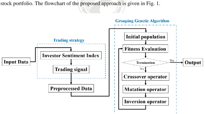
In this section, we will introduce our proposed approach, which uses two investor sentiment indices in the grouping genetic algorithm to obtain a diverse group stock portfolio. We first design some rules based on two sentiment indices to decide the buying and selling points of all the input stocks. These stock price data with buying and selling points are then sent to the proposed based approach for obtaining a best group stock portfolio. The proposed GGA-based approach will use the sentiment indices and the other factors in its fitness to evaluate the chromosomes (possible group stock portfolios). After a predefined number of generations, the chromosome with the best fitness value at the last generation is output as the diverse group stock portfolio. The flowchart of the proposed approach is given in Fig. 1.
Fig. 1 shows that the input data is preprocessed by trading strategy generated from investor sentiment index and trading signal. And, it puts the preprocess data into the grouping genetic algorithm to produce the best derived diverse GSPs with investor sentiment index. The components of the proposed approach are described as follows.
3.1 Data Preprocessing: Trading Strategy
For considering the sentiment factor in the proposed GGA-base approach for finding a good group stock portfolio, we first transform the input stock price sequences to the ones with sentiment considered. We design some rules based on two sentiment indices to decide the buying and selling points of all the input stocks.
Most of the portfolio research topics focus on how to find a high-risk and low-risk portfolio; however, little research is proposed to provide users with trading time points of the stock portfolio. In this study, we provide users with trading timings for each trading period. For instance, we assign the trading period from 2014 to 2016. With this research, we accurately informed consumers to buy the stock on February 3, 2014, and sell it on December 24, 2016. What is more, this study still retains the advantages of high-risk and low-risk of traditional stock portfolios.
In this study, the decision rules for determining the timing of buying or selling the stocks are based on the investor sentiment index. In the previous chapter, there are many indices that can reflect the investor's sentiment, called investor sentiment index. After filtering, we choose the research [41] to provide investor sentiment indicators as the basis for this study. There are three reasons for selecting the investor sentiment indices. First, the sentiment indices provided by the paper apply to the Taiwan stock market and it consists with the data used in this paper. Due to the different rules of the transaction, the floating price of the stock in different regions
will be different, and the impact of investor sentiment indices will also be affected. Therefore, selecting the same range of research as our paper is important. Second, the formulas for investor sentiment indices are clear and easy to understand. Too complicated formulas not only difficult to directly express its meaning but also cause the overlong operation time. Third, the indices are designed based on the behavior of retail investors. In Taiwan, retail investors' trading volume accounts for 70% of Taiwan's overall trading volume for the stock market. Therefore, studying Taiwan's retail investors' behavior is more meaningful and persuasive. Next, we introduce the two investor sentiment indices used in this paper to reflect the investor's sentiment.
The first index is called Buy-Sell Imbalance (BSIt), which is defined as follows:
, t t t t t VS VB BSL BML BSI (1)
,
t t tV
BI
VB
(2).
t t tV
SI
VS
(3)The parameters in this formula are as follows: BMLt is the balance of margin loan of the
stock on the day t; BSLt is the balance stock loan of the stock on the day t; Vt is the trading
volume of the stock on the day t; BIt is the buying volume of institutional investors of the stock
on the day t; and SIt is the selling volume of institutional investors of the stock on the day t.
With these defined parameters, BSIt means the value of buy-sell imbalance of the stock on the
day t, VBt means the retail investors' buying volume of the stock on the day t, and VSt means
the retail investors' selling volume of the stock on the day t.
Then we explain the proper terms used. The margin loan is an investor’s behavior which means investor borrows money from securities dealer to buy the stock. In Taiwan, the securities
dealer will borrow 60% of the value of the stock to investors with good credit to purchase the stock. For example, we assign that the price of the stock is one hundred, and the value of the stock is one hundred thousand. It means that investors can only use forty thousand to hold the stock by margin loan. In general, investors expect that stock price will rise in the future, but the hands of the funds is not enough; then they pay a part of the margin to securities dealer to borrow money for buying stock, and then wait for an opportunity to sell the stock at high prices and earn low selling low spreads. In contrast to a margin loan, the stock loan means investors borrow stock from securities dealer to sell it. If investors expect that stock price will fall in the future, they can borrow stock from securities dealer to sell by the stock loan. The trading volume represents the total number of transactions including institutional investors and retail investors, where institutional investors include foreign investment institutions, investment trusts, and dealers. The retail investors represent the individual investor. Retailers are usually composed of low-income individual investors and characterized by less investment per person.
Next is an analysis the formula of BSIt. Above all, we focus on the fractions. On a stock
at the time t, the higher of the BMLt means the higher volume of investor borrowing money to
buy the stock. This phenomenon can be interpreted as the degree of investors expecting the stock to turn high is increasing. On the other hand, the higher the BSLt means the higher volume
of investor borrowing stock to sell the stock. Therefore, if the difference between BMIt and
BSLt is high, it means the degree of investors expecting the stock to rise is high too; in other
words, investors are optimistic about the stock. If the difference between BMIt and BSLt is low,
it means investors are pessimistic about the stock. Then, we focus on the denominator. The sum of VBt and VSt means the overall retail investors' trading volume of the stock at the time t. To
sum up, at time t, higher BSIt value means that the retail investors are more optimistic about
the stock.
defined as follows: , t t t Shares NDT DT (4)
where NDTt is the number of day-trades and Sharest is the outstanding shares. In the stock
market, the number of day-trades (NDTt) means investors’ twice trading behaviors (including
buy after sell or sell after buy) by margin loan and stock loan on the same day t on the same stock. For example, if a man buys (sells) a share of TSMC on December 12, 2016 by margin (stock) loan and sells (buys) it by stock (margin) loan on the same day, the number of day-trades of TSMC on December 12 adds one. The Sharest means the amount of stock that the
company offers to investors on the day t. Generally, the magnitude of the Sharest change is
extremely small. Only when the company makes a big change, the Sharest will be different.
Therefore, the Sharest is used to normalize NDTt.
Next is an analysis of the formula of DTt. When the DTt of the stock turns high, it means
more and more investors day-trade the stock on the same day t. Generally, most of the investors do not day-trade, only those who are particularly interested in the stock will do so. Thus it can be seen that there is a positive relation between DTt and the degree of investors’ interest in the
stock. However, the value of DTt does not represent the investor expecting the stock price to
rise or fall. For instance, if investors are expecting the stock price to rise, they may buy a stock by margin loan and sell it by stock loan on the same day, and that causes the DTt of the stock
to rise. Then, if investors are expecting the stock price to fall, they may sell a stock by stock loan and buy it by margin loan on the same day, and this behavior still causes the DTt of the
stock to turn high.
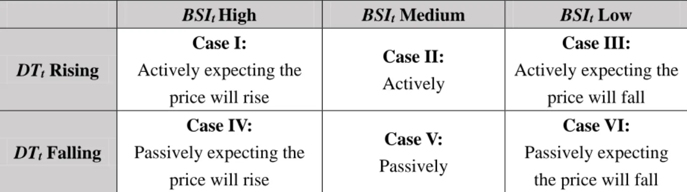
With these two investor sentiment indices, we divide the investor sentiments on a stock into six cases as follows:
Table 1. Six cases for the two investor sentiment indices.
BSIt High BSIt Medium BSIt Low
DTt Rising
Case I:
Actively expecting the price will rise
Case II: Actively
Case III: Actively expecting the
price will fall
DTt Falling
Case IV:
Passively expecting the price will rise
Case V: Passively
Case VI: Passively expecting
the price will fall
In Table 1, the investor sentiments are classified into six cases by the status of BSIt and
the change of DTt. We use the six cases in Table 1 to judge the stocks on every trading day. For
example, Case II reflects the active attitude of the investor on a stock. However, it does not give the rising or falling expectation of investors. Cases IV, V and IV reflect the investors holding the passive attitude to a stock. However, the passive attitude doesn’t affect the stock price. Therefore, Cases II, IV, V and VI can be ignored. On the contrary, the active attitude of investors to a stock will affect the stock price. Thus, we use Cases I and III to develop the trading strategy.
Next, we state how to determine the situations of DTt and BSIt for a stock on the day t.
DTt has two possible values: rising and falling. The way to identify the value of DTt is as
follows:
DTt Rise ↔ (DTt – DTt-1 > 0), and
DTt Fall ↔ (DTt – DTt-1 < 0).
For distinguishing the status of BSIt, the BSI thresholds are defined. The BSI thresholds
include Low BSI threshold and High BSI threshold as follows:
High BSI threshold = PR90(BSIt),
where PR10(BSIt) is the value which is at the PR10 from all 𝐵𝑆𝐼t value, and PR90(BSIt) is the
value which is at the PR90 from all 𝐵𝑆𝐼t value. The PR (percentile rank) value is a percentage
of scores in its frequency distribution that are equal to or lower than it. It is mostly used in the examination results above the rankings. For example, a score that is greater than or equal to
50% of the scores of people is said to be at the 50th percentile, where 50 is the percentile rank.
To practice the PR value, two steps should be implemented. They are assigned a string of numbers S as follows:
S = {12, 8, 2, 1, 17, 15, 4, 18, 9, 3, 11, 16, 10, 19, 5, 20, 14, 7, 13, 6}.
First, the string S is sorted from small to large. Then the new string S' is as follows:
S' = {1, 2, 3, 4, 5, 6, 7, 8, 9, 10, 11, 12, 13, 14, 15, 16, 17, 18, 19, 20}.
Then, we use the formula to calculate the PR value of every element in the string S'. The formula is as follows: N R PRvalue i i 50 100 100 , (5)
where Ri is the rank of element i, and N is the number of elements in the string S. Finally, we
get the PR value of every element in the string S. In this case, N is 20. The PR value of the element ‘2’ is 7, called PR7(S), because the rank of ‘2’ is 19. Similarly, proving that ‘3’ is
PR12(S), ‘4’ is PR17(S), …, ‘20’ is PR97(S). PR10(S) cannot be calculated due to the small
number of elements in the string S. Therefore, we choose the element which is larger than
PR10(S) and the closest one to PR10(S) to be the Low BSI threshold. The element ‘3’ is the Low BSI threshold. Similarly, we choose the element ‘19’ to be the High BSI threshold. With
which islarger than High BSI threshold, and the Low BSIt is the BSIt which is smaller than Low
BSI threshold.
Following that, we introduce the trading strategy in this proposed approach. Before defining the trading strategy, we combine Case I and Case III with buying and selling 46 company shares for finding the rules which maximize the stock return. The combination1 is, if Case I is true, buy the stock and if Case III is true, sell it. The combination2 is, if Case III is true, buy the stock and if Case I is true, sell it. Compare combination1 with combination2, find combination2, and make the overall stock more profitable than combination1. The reason for this phenomenon is likely to be that the investor sentiment experienced the lowest point is likely to rise and then drive the growth of stock prices. After the consolidation of the above information, the trading strategy is set up of this study. The trading strategy is composed of two rules as follows:
Rule 1: On a day t, if a stock’s BSIt is Low and DTt is rising, then buy the stock.
Rule 2: On a day t, if a stock’s BSIt is High and DTt is rising, then sell it.
Using the defined rules, the trading points are added to the original data. In this study, we define that the number of transaction on every stock is one. Therefore, we choose the first buying point and the last selling point to be the trading timing on this stock. By following this investor sentiment method, we get the Buy price and Sell price on every stock in the input data.
3.2 Components of the Proposed Approach
3.2.1 Encoding Scheme
We use a set S to represent n stocks, and denote them as {s1, s2, …, sn}. The number of
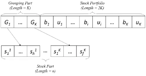
the groups is K. Then, the encoding scheme of the chromosome is defined as follows in Fig. 2.
Fig. 2. The encoding scheme of chromosome.
In Fig. 2, the chromosome consists of three parts including the grouping part, stock part, and stock portfolio. The number of groups in the grouping part is K. The results of the stock grouping are expressed in stock part. The sab means the stock is the a-th element in the group
b, where G1G2…Gk = {s11, s21, ..., sh1} {s12, s22, ..., sm2} ... {s1k, s2k, ..., sfk} = S, Gi and i j, Gi Gj = . Only one stock can be selected to compose the stock portfolio.
Therefore, it means that only K stocks may be selected from groups into the stock portfolio. In the stock portfolio, we use two genes to associate to each group. The two genes are bi and ui,
where bi is the threshold for deciding whether or not to buy the stock selected in the group Gi
and ui is the number of units purchased. If bi is greater than or equal to 0.5, it means a stock in
group Gi will be purchased ui units as part of a stock portfolio. Next, we use an example to
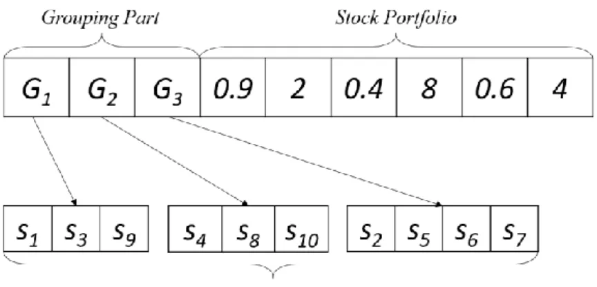
Example 1: There are ten stocks s1, s2, s3, ..., s10 and the number of group K is 3. The
chromosome is encoded as shown in Fig. 3:
Fig. 3. An example of encoding scheme.
In Fig. 3, ten stocks {s1, s2, s3, ..., s10} are divided into three groups G1,G2 and G3. The
allocation of stocks is {s1, s3, s9}for G1, {s4, s8, s10}for G2 and {s2, s5, s6, s7}for G3. Because
the values of b1 and b3 are larger than 0.5, it means that two stocks will be selected from G1
and G3 to compose a stock portfolio. To be more precise, one stock will be selected from {s1,
s3, s9} with two purchased units, and the other one will be selected from {s2, s5, s6, s7} with
four purchased units. In this example, it means that there are twelve (= 3*4) stock portfolios generated by this chromosome.
3.2.2 Initial Population
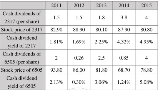
The strategy of generating initial population is important, because it reflects on the final optimization result. You et al. pointed out that a portfolio with cash dividend yield is better than a portfolio with types in the Taiwan stock market [39]. Therefore, choose cash dividend yields of stocks to frame the initial population in this proposed approach. Next, we use an example to explain this method for explaining the benefits of using cash dividend yield to generate initial population shown in Table 2. In Table 2, it shows cash dividends, stock price,
and cash dividend yield of two companies named Hon Hai Precision Industry Co., Ltd. (2317) and Formosa Petrochemical Corporation (6505).
Table 2. Cash dividend yields of two companies.
2011 2012 2013 2014 2015 Cash dividends of 2317 (per share) 1.5 1.5 1.8 3.8 4 Stock price of 2317 82.90 88.90 80.10 87.90 80.80 Cash dividend yield of 2317 1.81% 1.69% 2.25% 4.32% 4.95% Cash dividends of 6505 (per share) 2 0.26 2.5 0.85 4 Stock price of 6505 93.80 86.00 81.80 68.70 78.80 Cash dividend yield of 6505 2.13% 0.30% 3.06% 1.24% 5.08%
In Table 2, the cash dividends of 2317 are 1.5, 1.5, 1.8, 3.8 and 4, the stock prices of 2317 are 82.90, 88.90, 80.10, 87.90 and 80.80. Then, we calculate the cash dividend yields defined as that cash dividend divided by stock price. Therefore, the cash dividend yields of 2317 are 1.81%, 1.69%, 2.25%, 4.32% and 4.95%. In the same way, the cash dividend yields of 6505 are 2.13%, 0.30%, 3.06%, 1.24% and 5.08%. To compare the stability of 2317 and 6505, the standard deviation of each cash dividend yields is calculated. The standard deviation of 2317 is 1.35938, and the standard deviation of 6505 is 1.63947. As a result, we know 2317 is better than 6505 because the cash dividend yield of 2317 is stable. It means that buying 2317 can earn a stable income at low risk. Then, the cash dividend yields (yi) of n companies are shown in
Table 3.
Table 3. The cash dividend yield (yi) of companies.
s1 s2 si sn-1 sn
With the cash dividend yield (yi) of n companies, we use some existing techniques like
kNN and k-means clustering to divide n stocks into K groups. The average cash dividend of each group avgCDi is calculated. Then, we calculate the proportion of average cash dividend
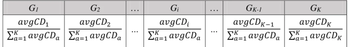
of each group to all groups, and the result is shown in Table 4.
Table 4. Proportion of average cash dividend of each group.
G1 G2 … Gi … GK-1 GK 𝑎𝑣𝑔𝐶𝐷1 ∑𝐾 𝑎𝑣𝑔𝐶𝐷𝑎 𝑎=1 𝑎𝑣𝑔𝐶𝐷2 ∑𝐾 𝑎𝑣𝑔𝐶𝐷𝑎 𝑎=1 … 𝑎𝑣𝑔𝐶𝐷𝑖 ∑𝐾 𝑎𝑣𝑔𝐶𝐷𝑎 𝑎=1 … 𝑎𝑣𝑔𝐶𝐷𝐾−1 ∑𝐾 𝑎𝑣𝑔𝐶𝐷𝑎 𝑎=1 𝑎𝑣𝑔𝐶𝐷𝐾 ∑𝐾 𝑎𝑣𝑔𝐶𝐷𝐾 𝑎=1
In Table 6, the proportions of the average cash dividend of each group are shown. It means that the probability of being selected in the stock portfolio of each group. For instance, if the
avgCD1 is larger than the avgCD2, it means that the probability of G1 being selected in the stock
portfolio is higher than G2 being selected in the stock portfolio. It can be seen that the larger
the average cash dividend of the group is, the larger the probability of a stock being chosen from the group to form the stock portfolio. By using this method, the quality of the initial population can be improved.
3.2.3 Fitness Evaluation
In this section, we introduce the fitness functions used in this study. The fitness functions are used to determine the quality of the chromosome. In the law of nature, the fitness functions are equivalent to the conditions of natural selection. It is very important to define the appropriate fitness function because it affects the results of the entire algorithm. Since the goal of this study is to mine the diverse group stock portfolio, the fitness function is used to score the chromosome and decide whether to retain it. In this paper, the fitness functions are designed
based on the risk of investor sentiment, portfolio satisfaction, group balance, price balance, unit balance and diversity factor. The following describes the five fitness functions used in this article.
The risk of investor sentiment (RIS) is used to assess the risk of the stock using the investor sentiment strategy trading. After using investor sentiment index, we get the trading signals which decide the trading timing. In general, the trading signals will produce many transactions. Although the trading strategy in this study only takes a transaction to determine trading timing on each stock, we need all the difference of trading price (DTP) in transaction records by using trading signals to calculate RIS. To practice RIS, there are three main steps that should be followed. The first step is finding the minimal difference of trading price (minDTPi) on each
stock, where i represents the stocks. The second step is finding the maximum minDTPi named
MAXminDTP and the minimal minDTPi named MINminDTP from all stocks. The third step is
normalizing the minDTPi to the range [0, 1] and getting the nomalDTP(si) on each stock by the
following formula: . min min min min ) ( DTP MIN DTP MAX DTP MIN DTP s nomalDTP i i (6)
Then, we calculate the subRIS(SPp) by the following formula:
* , ) ( 1 i n i i p nomalDTP s u SP subRIS
(7)where ui is the number of purchased units of stock si, and subPS(SPp) is the RIS of the p-th
stock portfolio SPp. Finally, the RIS(Cq) is calculated by the following formula:
, / ) P ( ) ( 1
NC p p q subRIS S NC C RIS (8)Take an example to explain this method. Assume there are five companies {company A,
company B, company C, company D, company E}, and the transaction date is from 2011/1/3 to
2011/1/28. The trading information of company A is shown in Table 5.
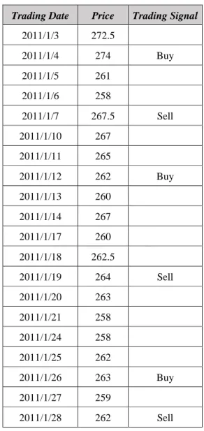
Table 5. The price and trading signals.
Trading Date Price Trading Signal
2011/1/3 272.5 2011/1/4 274 Buy 2011/1/5 261 2011/1/6 258 2011/1/7 267.5 Sell 2011/1/10 267 2011/1/11 265 2011/1/12 262 Buy 2011/1/13 260 2011/1/14 267 2011/1/17 260 2011/1/18 262.5 2011/1/19 264 Sell 2011/1/20 263 2011/1/21 258 2011/1/24 258 2011/1/25 262 2011/1/26 263 Buy 2011/1/27 259 2011/1/28 262 Sell
In Table 5, the price is the closing price on every trading date, and the trading signals are produced from the trading strategy described in section 4.1. There are three trading times from 2011/1/3 to 2011/1/28. The first DTP is -6.5 (267.5-274). It means that investors buy this stock on 2011/1/4, sell it on 2011/1/7 and lose 6.5 in this transaction. In the same way, the DTPs of
three transactions are -6.5, 2 and -1. Obviously, the minDTPA is -6.5, and so on. Then, we get
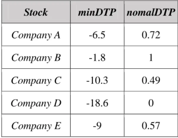
the minDTP of five companies. The five companies’ minDTP and the nomalDTP are shown in Table 6.
Table 6. The minDTP and the nomalDTP on five companies.
Stock minDTP nomalDTP
Company A -6.5 0.72
Company B -1.8 1
Company C -10.3 0.49
Company D -18.6 0
Company E -9 0.57
In Table 6, the MAXminDTP is -1.8, and the MINminDTP is -18.6. Finally, the subRIS of each stock is calculated by the formula 7. Company B has the largest nomalDTP from all companies, and it means that Company B has the maximum difference of trading price from all companies. In other words, Company B has the highest return under the investor sentiment strategy. If Company B is selected into the stock portfolio in the chromosome, the quality of the chromosome is higher than the chromosome which did not select Company B into stock portfolio under the same conditions.
The portfolio satisfaction is used to assess the profit and requests given by users of a chromosome. When a chromosome has high portfolio satisfaction, it means stock portfolios generated from a chromosome can get high returns from stock portfolios and satisfy objective and subjective criteria given by users. Formally, the portfolio satisfaction of a chromosome Cq
, / ) P ( ) (Cq
NCp1subPS S p NC PS (9)where NC is the number of stock portfolios generated from chromosome Cq, and subPS(SPp)
is the portfolio satisfaction of the p-th stock portfolio. The formula of subPS(SPp) is as follows:
) ( ) ( ) ( p p p SP y suitabilit SP ROI SP subPS , (10)
where ROI(SPP) is the profit of the stock portfolio in SPp, which is calculated by the following
formula:
n i i i i i i b i s p SP SP u Div u Tax SP ROI( ) 1 ( ( ) ())* ()* ( ) , (11)where ui is the number of purchased units of stock si, SPs(i) is the selling price of si, SPb(i) is the
buying price of si, Div(i) is the cash dividend of si and the Tax(i) is the transaction tax of si. In
Taiwan, the transaction tax consists of the handling fee and the securities transactions tax. When investors buy the stock, investors have to pay the buying handling fee to the securities company. When investors sell the stock, investors have to pay the selling handling fee and the securities transactions tax to securities company. The formula of Tax(i) is as follows:
%). 3 . 0 * % 1425 . 0 * % 1425 . 0 * ( * ( ) () () ) ( i s i s i b i i SP SP SP u Tax (12)
The suitability(SPp) is used to evaluate whether the stock portfolio meets the subjective
criteria given by investors. The suitability(SPp) includes the investment capital penalty (ICP)
and portfolio penalty (PP). The ICP is used to measure the satisfaction degree of investment in a portfoliorelative to the predefined maximum investment. The PP is used to measure the satisfaction degree of the number of purchased stocks in a portfolio relative to the predefined maximum number of purchased stocks. The ICP(SP) is defined as:
, Inves max Cap if , Inves max Cap ; Cap Inves max if , Cap Inves max S ICP p p p p P)= ( (13)
where CapP is the investment capital of SP and maxInves is the predefined maximum
investment. The PP(SP) is defined as:
, numCom numCom if , numCom numCom ; numCom numCom if , numCom numCom S PP p P p P P)= ( (14)
where numComP is the number of purchased stocks of SP and numCom is the predefined
maximum number of purchased stocks. Hence, the suitability(SP) is defined as:
). ( ) ( ) (Sp ICP Sp PP Sp y suitabilit (15)
The group balance is used to make the groups have the number of stocks as similar as possible. For this goal, the concept of entropy is added in this fitness function. The group balance for a chromosome Cq is defined by the following formula:
, log ) ( 1
K i i i q N G N G C GB (16)where |Gi| represents the number of stocks in the i-th group. Hence, if a chromosome has a
large group balance value, it means that numbers of stocks in groups are similar.
The unit balance is designed to avoid generating too large or too small purchased unit ui
for a group and make sure the purchased units of groups can range from the predefined [minPurchasedUnit, maxPurchasedUnit]. The unit balance is defined by the following formula:
. , 1 ; 0 if , 15 . 1 ; if , 4 . 1 ) ( 1 1 otherwise U K U C UB ki i k i i q (17)where K is the number of groups and Ui means whether the purchased unit ui of group Gi is in
the predefined range. If the purchased unit is in the range [minPurchasedUnit,
maxPurchasedUnit], Ui is 1. Otherwise, Ui is -1. When UB(Cq) is 1.4, it means that the
purchased units of all groups are in the predefined range. If UB(Cq) is 1.15, it indicates some
purchased units are not in the predefined range. Otherwise, UB(Cq) is 1.
The price balance is designed to make the price of every stock in the same group as similar as possible. The price balance is defined by the following formula:
), | | | | log | | | | , 1 ( ) ( 1 1
k i n j i j i j q G Sec G Sec Max C PB (18)where Secj is the stock price section which is defined by user, |Secj| is the number of stocks in
j-th section and |Gi| is the number of stocks in group Gi.
The diversity factor is used to increase the diversity of stocks in the same group. The diversity factor is defined by the following formula:
, ) ( 1 K D C DF K i q i q
(19)where Diqis the diversity value of group Gi in chromosome Cq and K is the number of groups.
The Diqis calculated by the following formula:
, ) , ( , , i t h and G s s t h q i G s s dissMatrix D h t i
(20)where sh and st are two stocks in the same group Gi, and dissMatrix(sh, st) is the difference
between sh and st. The dissMatrix(sh, st) is calculated by the following formula:
, ) , ( 1
m l l t h s d s dissMatrix (21)where dl is used to assess the difference of an attribute between two stocks and m is the
number of attributes used to calculate the diversity of GSP. In the proposed approach, the two attributes, industry category ah1 and company capital ah2, are used. The distance d1 of two
stocks is one when ah1 is not equal to at1, which means sh and st are in different categories.
Otherwise, d1 is zero. The distance d2 is calculated by the following formula:
. , 1 ; 00 4 200 , 3 2 ; 00 2 100 , 3 1 ; 100 , 0 2 2 2 2 2 2 2 otherwise a a if a a if a a if d t h t h t h (22)
This formula shows that if the capital difference of stocks sh and st is between 0 and 10
billion, the score is zero. If the capital difference of stocks sh and st is between 10 and 20 billion,
the score is 1/3. If the capital difference of stocks sh and st is between 20 and 40 billion, the
score is 2/3. Otherwise, the score is 1.
With the above description, the final fitness functions are defined by the formula:
, ) ( * ) ( * ) ( * ) ( ) ( 1 q q q q q RIS C PS C GBC DF C C f (23) , ) ( ) ( * ) ( * ) ( * ) ( * ) ( ) ( 2 q q q q q q q C PB C DF C UB C GB C PS C RIS C f (24)
3.2.4 Genetic Operation
In this section, genetic operations are described, including crossover, mutation and inversion operations. The crossover operations are designed for grouping part and stock portfolio, the mutation operations are designed for stock part and stock portfolio, and the inversion operation is designed for the grouping part.
3.2.4.1 Crossover
The first phase of crossover operation is on the group part and the second part is on the stock portfolio part. In the grouping part, it randomly selects chromosome CA to be the base
chromosome, and inserts some groups from another chromosome CB. Then, it deletes the
duplicate stocks from the new chromosome Cnew. Formally, it assumes CA as the base
chromosome and CB as the inserted chromosome as follows:
A K A p A p A A A G G G G G C 1 2... 1... and
where p is the point of insertion, s is the starting group in the inserted segment, and m is the number of inserted segments. The parameters p, s, and m are generated randomly. The new chromosome Cnew is generated as follows:
i[1, K].
The will be removed if . Then, there are three situations after elimination process including Case (1): |Cnew| < K, Case (2): |Cnew| = K, and Case (3): |Cnew| > K. The |Cnew| is the number of non-empty groups in the new chromosome. The Case (2) satisfies the definition of chromosome, and the others need to be adjusted. In the following, adjustment of Cases (1) and (3) are stated.
, G ... G G ... G G C KB B m s B s B B B 1 2 1 , G ... G G ... G G ... G G Cnew 1A' 2A' pA' sB sBm1 pA' KA' C G (G G ... GsBm ), B s B s A i ' A i 1 1 ' A i C CiA'
Case (1): |Cnew| < K
In this case, it represents that the new groups should be added to satisfy the constraint. Therefore, a new group Gi is randomly selected from . Then, the group
Gi will be split into two subgroups. This process is repeated until the grouping part has K
non-empty groups.
Case (3): |Cnew| > K
In this case, it means that some groups should be removed. The roulette wheel selection strategy is used to select the groups to remove. When a group is picked for removal, the stocks inside it are reappointed to other groups randomly. If a group has few number of stocks, it has large probability to be removed. In the stock portfolio part, we use a one-point crossover in the proposed approach. The one-point crossover operator generates two new offspring from their parents with a random crossover location d. Of course, more sophisticated crossover operations could be utilized.
3.2.4.2 Mutation and Inversion
The two-phase mutation operation is designed in this section. The first phase of the mutation operation is for the stock part and the second phase is for the stock portfolio part. In the first part, the two groups are selected randomly, where the number of stocks of each group is larger than 1. Then, the mutation operator will reassign a stock into another group. In the second phase, we use a one-point mutation in this approach. A gene is selected to mutate. There are two cases in this step. The first case is that if the odd gene in the stock portfolio part is selected, it changes the value from [0.5, 1] to [0, 0.5] or from [0, 0.5] to [0.5, 1]. The second
G G , K N G | Gi i i
case is that the even gene in the stock portfolio part is picked, it randomly generates a value from the range [1, maxUnit] to replace original one.
The inversion operator is to make the crossover operator to generate various combinations of groups to exchange between two parents. In the proposed approach, the rearrangement is done randomly for this target.