Design and control of a novel plane Maglev system based on analyzing magnetic force

Proceedings of the 5% World Congress on Intelligent Control and Automation, June 15-19, 2004, Hangzhou, P.R. China

Design and Control of a Novel Plane Maglev System

Based on Analyzing Magnetic Force

Ming-Chiuan Shiu"', Mei-Yung Chen", Shin-Guang Huang'and Li-Chen Fuqb

aDepartment of Electrical Engineering, National Taiwan University bDepartment of Computer Science and Information Engineering

National Taiwan University

'"%o.l, Sec.4, Roosevelt Road, Taipei 106, Taiwan, China

bE4nail: [email protected]

'Department of Electrical Engineering, Hsiuping Institute of Technology 'N0.11, Gungye Road, Dali City, Taichung 412, Taiwan, China

E-mail [email protected] "

Abstract

-

In this paper, a novel 6-DOF magnetic levitation (Maglev) system is proposed. As a result of using the cylindrical solenoid and rectangular coils as actuators, we thought analysis of magnetic forces inside the both kinds of coil form the main basis of designing our system. In this system, both new mechanical structure and adaptive control algorithm are developed. Structurally, totally there are eight permanent magnets (PMS) attached to the carrier, whereas there are eight coils respectively mounted on a fired base. After analyzing the magnetic force characteristics between permanent magnets and coils, and detailed studied the general model of this system with full 6DOFs is therefore derived and analyzed. Next, an adaptive controller is developed for such a system to deal with the unknown parameters with the objective of precision positioning. From the experimental results, satisfactory performances including regulation accuracy and control stiffness have been demonstrated.

Index Terms

-

Magnetic force, Maglev, Permanent magnet,

Adaptive controller,.

I. INTRODUCTION

.

With, the progress of the industrial technologies, the high-precision positioning system plays an important role in various high-tech fields. To meet these challenging needs, more stringent manufacturing processes and advanced fabrication equipments, therefore, should be developed. In traditional mechanical actuators, mostly the piezoelectric actuators [1][2] only handle the small moving range, the ball-screws cause disturbances and backlash due to roughness of the bearing elements [3][4], and linear motors have ripple effect in a motion stroke. It is generally believed that magnetic levitation system not only achieves advantages that the previous two actuators possess but even overcome their shortcomings as well.

Based on the design theories and experience for developing dual-axis Maglev guiding systems and planar maglev positioning system [5][6], a new planar Maglev system is proposed in this paper. There are eight PMs attached to the moving part, which is the so-called camer, whereas there are eight coils respectively mounted on a fixed base. Four of these eight coils are arranged in the bottom, which

mainly generate levitating forces as well as torques around X-

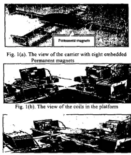
and Y-axis. On the other hand, the four lateral-coils with rectangle shaped mainly produce lateral forces and torque around Z-axis as well. The conceptual configuration and photograph of this system is shown in Fig. l(a), Fig. I(b) and Fig. 2, respectively.

In this paper, first, the magnetic force characteristics are analyzed. Then, the dynamic model with full 6DOFs is derived from it. Also, an adaptive controller that deals with unknown parameters is proposed to control the camer at the desired target point. To demonstrate the performance of the entire system, experimental results are provided for verification. The organization of this paper is as follows. The detailed description of the complete dynamics that including the magnetic force characteristics will be given in Section 11.

And Section 111 concentrates on the system modelling and controller design. Section IV is about the experimental results

as well as snme discussions. Finally, conclusions are given in section V.

Fig. 1 (a). The view of the carrier with eight embedded

Fig. l(b). The view of the coils in the platform

1-

11. MAGNETIC FORCE DISSEClTNG

About this system, it can he regarded composed of eight sub-systems. The upper four sub-systems and the lower four have different pairs of coil and PM. They are rectangular and cylindrical, respectively. To model this system, the interactions between coil and PM become a very important issue. Thus in this section we begin with two approaches, which are introduced to analyze these interactions. Furthermore, this modeling result will then he integrated to develop the general model of the hereby proposal.

A . Analysis ofMagnetic Force Characteristics

First, we try to model the interactions from the analytic approach by utilizing several useful fundamental theorems in electromagnetics. The force and torque exerted on a PM, which is exposed in an external magnetic field

i?

,

can be obtained from the Lorentz force form

P =(%.

V ) & H , ( 1 )

where Ct denotes the dipole moment of the PM and p o

is

the permeability of free space which is equal to 4 z x ( H h ) . In this system, it is assumed that each

PM

can be viewed as a single magnetic dipole moment with the direction perpendicular to its surface. Therefore, how to derive the magnetic field becomes an important task in this research.

From Biof-Savarf Law [7], the magnetic field H can he expressed as:

( 3 )

where j is the current density, f ' is the source coordinate, F represents the observer coordinate, <,, is a unit vector directed from F ' to F , and dv' is a infinitesimal cube of the current source.

B. Magnetic Field Inside the

Coi

Generally speaking, we need to have sufficient understanding about the property of every element device before we can assemble them into our MagLev system. What is shown in Fig. 3 is a rectangular coil with inner-length a, inner-width b; height h and current I (=1 A). Apparently, the origin of the coordinate attached to the coil is at the center of

the coil's bottom.

First of all, we should explore the property of the ~~ ~

magnetic field inside the coil. By using an auxiliary software,

we can perform 3D-simulation of the magnetic field on the xy-plane at z=O.Olmeter or at z=O.O245meter over the range (x:-0,025

+

0.025 meter, y:-0.025 + O.O25meter), where

Bx means the part of

B

in the x-direction, By means the part of

B

in the y-direction, Bz means the part of B in the z-direction, and the unit of the magnetic flux (B) is Gauss.

Fig. 4. Bx in the xy-plane (z=O.OImeter)

Fig. 5. Bx in the ny-plane (d.0245meter)

Fig. 6. By in the xy-plane (z=O.Olmeter)

Fig. 7. By in the xy-plane(~0.0245meter))

Fig. 8 . Bz in the xy-plane (z=O.Olmeter

z(r~-plansl Mho"" O.Olm O.025m(cFsrr) 0.wm o.Osm(lop)

Bx High

-

Low Low

-

Hieh

3 Hfgh

-

Low Lou

-

High

B i Low

-

Hlgb High

-

Low

-

Fig. 10. Fn in the xy-plane (z=O.Olmeter)

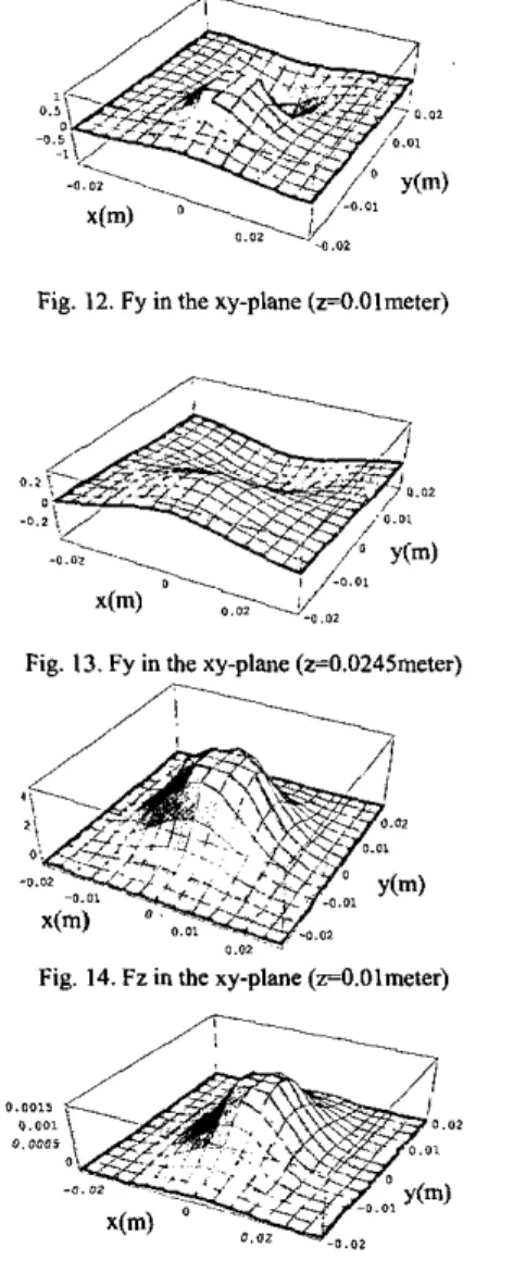
Fig. 12. Fy in the xy-plane (r=.Olmeter)

- 0 .

Fig. 13. Fy in the xy-plane (~0.0245meter)

Fig. 14. Fz in the xy-plane (z=O.Olmeter)

!

Fig. IS. Fz in the xy-plane(~0.024Smeter)

On the other hand, we can extract more important meanings from the force simulations by investigating the force distribution on the xz-planes at y=Ometer over the range

( x : -0.03 --f 0.03mete1, z: O.Olb+O.O4 meter, m = I S Am' ,

P I A ) as shown in Fig. 16 and 17. It can he found that when the location of PM is above or helow the center of coil, it will he attracted

to

the center referring to Fig. 16. In summary, the pair of the coil and a

PM

has

a

stahle equilibrium point at the center of the coil under the following conditions:

I. if the vector of dipole moment (m) is in the +Z direction,

2. if the vector of dipole moment (m) is in the -z direction, and But when the location of PM is above or below the center and I is in the counterclockwise direction;

I is in the clockwise direction.

of coil, it will be repelled away the center referring to Fig. 17. Fig. 11. Fx in the xy-plane (z=O.O245meter)

Fig. 16. Fz in Le xz-plane (y=Ometer)

Fig. 17. R in the xz-plane (y=Ometer)

To sum up, the pair of a coil and a PM has an unstable equilibrium point at the center of coil under the following conditions:

1. if the vector of dipole moment (m) is in the -z direction, and

2. if the vector of dipole moment (m) is in the h direction, In our developed system, we will set up the positioning force and levitation force exerted to the carrier basically using repulsion mechanism as will be explained in the following:

Here, four PMs embedded at the bottom of the carrier are used to counteract the weight of the canier. But, besides the levitation forces there will be unstable lateral forces (Fx, Fy)

coming along to make the camer statically unstable in the lateral direction. So, we design the carrier such that there is a PM embedded in the foot plate of each extended bar and the total four PMs together with the rectangular coils will sufficiently provide the lateral control forces to hold the carrier still. In this Maglev positioning system, generation of levitation forces will usually be at the price of destabilization in lateral directions (when the carrier is not right at the equilibrium state).

After we have carefully described the mechanism of the Maglev system, what is left for us is to develop an appropriate control, which not only can levitate the carrier but also will position the canier precisely at the pre-specified location or will move it following the desired speed and trajectory.

I is in the counterclockwise direction; and I is in the clockwise direction.

111. SYSTEM MODELING

In order to realize such high-precision positioning system, we must control not only the translation but also the attitude of the carrier. To this end, a complete analytical model will be derived first, which includes two lateral DOFs, one propulsion DOF and three attitude DOFs. Before we derive the model, several technical assumptions must be made.

Assumptions:

1.Every PM (permanent magnet) is considered as one single dipole carrying the same magnetic dipole moment and is located at the center of each PM.

2.Tbese PMs do not have any influence among one another. 3.These coils are arranged such that the mutual inductance 4.Both the carrier and platform are rigid bodies

After these assumptions are validated, the complex analysis of

the overall MagLev system will become simpler.

A . Controller Design and Stabilig Analysis

To simplify our notations from here on, we will drop the differential symbol “

S

” and abuse the notations by

identifying the variable 6 X with X and doing the same to all others. Under this circumstance, we further redefine the control inputs u10 u8 as U, = I , , u , = l s r u 3 = l c ,

uA = I,,u, = I , , u , = l , , u , = l , , u , =I,. As a result of this

notational simplification, the plant model now becomes: among them can be negligible.

i=

K,,X+ K,,Y+ K,,Z+ K , , J J + K,,$J+ K,,B+ K,,u,

+ K,& +K,cu, + K,,% + %FU5 +KIP% +K,& +K,”%

Y = K J + K,,Y

+

K,,Z

+

K , , y + K,,(+ K,,B+ Kip,

+K,,u,+K,cu,+K,,u,+K,,u,+K,,u,+K~tiU,

+ K d *

z

= K,,x+ K,,.Y

+

K ~ ~ Z

+

K,,v+ K,,(+ K,,B+ K,,~,

+4,%

+K,& +K,D% +K,& +K,& +K3&

+K,H%

(4)

~=K~,X+K,,Y+K,,Z+K,,W+K,,(+K,,B+K~~B+K~~U* + K 4 D u 4 + K 4 E u 5 + K 4 F u 6 + K 4 & 7 + K 4 H u 8

4

= K,,X+K,,Y

+

K&

+K,,y/+ $,)+ K,,B+ &,U,

+K5Cu3 + K 5 E u 5 + K 5 F u 6 + K 5 G u 7 + K 5 H u 8

e =

K,,x+K,,Y

+

K ~ ~ Z

+

K,,Y+K,,C+ K,B+K,,u,

+Kmug + K c u , + K m u ,

Note that all the above resulting linear coefficients can be found in [SI.

B. Adaptive Controller Design

in our final plant model, (4) can be rewritten as:

'Xl Y

z

eu

4j

e ]

-G

K,, K,, K,, K,, K,,

4,

K,,1

4"

4,

4,

K 2 D

4,

4, 4,

K*"

4,

K,, K,,

4,

K,, K,, K,, K 3 H 0 K 4 B 0 K4D

4,

K4F K 4 G K4" K," 0 K5c 0

4, 4,

K5, K I H . K 6 ~ 4 8 &C Kc, C. Stability Analysis

function candidate V as follows:

To find out the adaptive law, we first define a Lyapunov

1 1 1 2 2 2 1 V = - S ' S + - Y ( ~ G ; ' ( ~ ] + - O f ( ~ G ~ ' ( ~ ] (11)

+j%i)r

GLIG)l

where G,,G, and G, are all positive definite diagonal matrices. To assess the boundedness as well as convergence of all the involved errors, we will try to evaluate the time derivative of the function V in the following:

, Y U1 g2 U4 g, U5 g4 U6 g5 %

+

.U8

1

Substitute S from (9) into (12) to yield

k = S ~ [ ~ + S U + g - A , ~ + Y ( ~ ' G ~ ' ( ~ ] +t((B)'G<' ($)l+~f@)~G;'

(g)]

(13)

-'

-1 L ' = - S ~ l \ , S + S ~ ~ + S ' ~ U + S ' g + O f ( ( A ) CA (A)] G;' ($)]+Of(i$G;'

G)]

. .

So that, the obvious choice for

2,

d

andh to make

k

negative is

~-

A = - A = G,SE', where G, = diug(x,,,X,, ,..., Z A G ) B = -B = G,SUT , where G, = diag(xsI,Xs2, ...,

x e s )

i

=

-g

= G8S

,

where Gp = diag(x,,,X,,

,...,

x g 6 )

,

~-

. .

so that (13) can be further simplified as:

V = -STA,S 5 0 . (14)

Based on (11) and (14) and according to the Lyapunov stability theory, we can conclude that

S,i,E

und are all bounded, and SE

&

. Refemng to (IO), we can find that

SE

L- and hence

S

is uniformly continuous, which together with the fact that SE L2 will readily imply that (SI-tO as

f + m by Barbalat's Lemma 193. It is, however, worth mentioning that

2

, E and

g

may not converge to their true values A

,

B and g

.

Of course, if the so-called persistent excitation (PE) condition can be satisfied, estimates should he able to converge to their true values asymptotically. Under that circumstance, the input command U readily becomes what we derive as if all the parameters were known. Regardless of the failure of parameter convergence, the error E and E will approach to zero asymptotically. In other words, six state

errors and their time derivatives will all converge to zero asymptotically. As a consequence, the objective in our developed system can be fulfilled by the formerly designed controller.

IV. EXPERIMENT RESULTS

The experiment hardware, including the main body, sensor system, deriver system and controller hardware, will he described here. A number of experiment results, including the regulation and positioning will also he provided in this section to demonstrate performance of this system with the controller presented in section 111.

In our experiment results as Fig.18-29, not only the performance of regulation but also the positioning has been achieved as desired goals. Besides, all the states will converge to their desired values with precision, and these experiment results are quite consistent with the results from numerical simulations.

REFERENCES

[I] Sitti, M. and Hashimoto, H., “Two-dimensional fine particle positioning using a piezoresistive cantilever as a microlnano-manipulatof’, 1999 IEEE lnrernorionol Conference on Roborics and Automotion, Vol. 4,

1999. pp. 2129 -2135.

Hector M. Gutierrez, Paul 1. Ro. ”Sliding-Mode Control of a Nonlinear- Input System: Application to a Magnetically Levitated Fast-Tool Servo”, IEEE Tmn. on Indusrriol Electronics ,Vol. 45, no. 6, 1998, pp. 921 -927.

Li Xu and Bin Yoo, “Adaptive robust precision motion Control of linear motors with negligible elechical dynamics: theory and experiments”, IEEE/ASME Trm. on Mechnrronicr, Vol. 6 Issue: 4 , 2001, pp. 444 - 452.

Pa;-Yi Huang, Yung-Yew Chen ond Min-Shin Chen ”Position-dependent friction compensation for ballscrew tables”, Proceedings of rhe 1998 IEEE Inrernorionnl Conference on Conrrof Applicarions, Vol. 2 , 1998, pp. 863 -867.

Chen, M. Y., Wu, K. N. and Fu, L. C., “Design, Implementation and Self-hming Adaptive Control of a Maglev Guiding System”, Mecharronic, 2000, pp. 215-237.

Shiu, M. C.;” Design and Control of a Novel Planar Maglev Positioning System.” Master thesis. The National Taiwan University, Taiwan, China, 121 131 [4] [ 5 ] [6] 7nnl _“I..

Finally, the regulation and positioning errors are within [7] David, J. G., Inrroduction IO Electro<vnomics. Prentice-Hall, ~nc.,

IOOpm, which are yet to he further improved. Englewoad Cliffs, New Jersey, 1981.

Huang, S . G.;” Design Control and Experiment of a Novel Precise Maglev Positioning System.’’ Master thesis. The National Taiwan Univeniw. Taiwan. China. 2002.

[SI

V. CONCLUSION

In this paper, we proposed a novel planar Maglev positioning system. This maglev system can be readily used in a clean room, since it will not generate wearing particles and no lubrication is required. Furthermore, there is no mechanical contact between the moving part and the stators. This design is also highly suitable for vacuum environments, since the heat generated in the motors in the fixed frame.

Then, the dynamics of our Maglev system have been thoroughly analyzed and its mathematical model with complete six DOFs (degree-of freedoms) is also detailed derived. By this, we can particularly understand the dynamics between a levitated free body and platform of guiding system.

The system is treated as a MIMO system, and an adaptive controller has been designed to regulate the six DOFs to a precision extent. Finally, satisfactory performance of precision positioning motion can be obtained in the actual experiments. The inexact setup of mechanism and the inaccurate precision of sensors will result in the error in our system performance. Based on the process of experiment, we find that the improvement of system performance is possible if the more high-precision sensors, the exacter mechanism and the more advanced control is practiced.

The hereby-developed Maglev planar positioning system is novel in that it can provide planar dual-axis motion capability, which involves only pure magnetic forces. Functionally, such mechanism behaviors just like a planar XY table with high precision.

To sum up, a high-precision novel planar Maglev positioning system has been successfully put into practice there.

ACKNOWLEDGMENT

This research is sponsored by National Science Council, Taiwan, China, under the grant no. NSC-90-2.213-E-003-054.

~_

[9] Jean-Jacques E. Slatine, Weiping Li., Applied nonlinear control, Prentice Hall, 1990. 4 p,-..d-.-,.b.- a “,.i.

*...

i

,

_._..I ... ... ..,.. . . . . . . . ... , ,

IjJ

:3

_{.-! ... ...}

_{. . .}

_!.

Fig.19. Regulation response on

-,

Fig.18. Regulation response an

X-axis. Y-axis

.~~

Fig.20. Regulation response on Z-axis. Fig.21. _... F%t:%”&egulation

... i

.,,,

i

1

...

.---....-.

{!I>”

1

’ .‘f

i

.? ... ... ,....,

!.

.L

i... -vz2 ~ ! .

.j

,,,.

I --*bit ,,,- ... ... ...

-

Fig.22. Yaw regulation. Fig.23. Roll regulatioo ... ... ./ ,.,,. 1 I-.._,_._ . .

>-~’.;.:=:

... ::-.:,.

I

..:,

.

I

.I’J

... f ~~ ... ~~ .. .r_; _...., ... , ~ J -X _i...

..

_:. .. _...

i.

Fig.24. Positioning response on Fig.25. Positioning response on

X-axis. Y-axis . . . ... ... _... . . . i .( ../ ..:

..

., .. ’-. ... !. Fig.26. Positioning response on

Z-axis.

... ...

:!I \

.,I ... , ~ ~... ~ .i .

Fig.27. Positioning response for pitch

... ...

__

...

.!. ... ... _- .:

Fig.28. Positioning response for yaw. Fig.29. Positioning response for roll ?