A two-phase navigation system for mobile robots in dynamic environments

(1)

A

Two-Phase Navigation System for Mobile Robots

in Dynamic Environments

Tsai-Yu Chang, Szu-Wen Kuo and Jane Yung-jen Hsu

Department of Computer Science and Information Engineering

National Taiwan University Taipei, Taiwan 106, R.O.C. yjhsuQcsie.ntu.edu.ta

Abstract

This paper presents a n implemented navigation s y s t e m f o r mobile robots in d y n a m i c environ- m e n t s . In order t o take advantage of existing knowledge of t h e world and t o deal w i t h u n k n o w n obstacles in real t i m e , our s y s t e m divides m o t i o n planning i n t o global p a t h p l a n n i n g and local re- active navigation. T h e f o r m e r u s e s genetic algo- rithm m e t h o d s t o find a collision-free path; t h e latter is i m p l e m e n t e d using n e u r a l n e t w o r k tech- n i q u e s t o track t h e p a t h generated by t h e global p l a n n e r while avoiding u n k n o w n obstacles o n t h e w a y . A s a result, t h e s y s t e m c a n adapt t o dy- n a m i c e n v i r o n m e n t a l changes. Our e z p e r i m e n t s , both in s i m u l a t i o n a n d o n a real robot, showed t h a t t h e s y s t e m c a n find a reasonably good free p a t h an a f r a c t i o n of t h e t i m e n e c e s s a y t o f i n d a n o p t i m a l free p a t h , a n d it c a n effectively achieve its goal configurations w i t h o u t collision.

1 Introduction

A mobile robot accomplishes tasks by moving in the real world. M o t i o n p l a n n i n g , namely, deciding what motions to perform in order to achieve goal arrangements of phys- ical objects, is one of the most important capabilities for a mobile robot. Although it may seem like a relatively simple job for humans, motion planning requires sophis- ticated integration of reasoning, perception and control. Many techniques for performing path planning and navigation have been developed over the years. On the one hand, most planning methods assume complete knowledge of the environment, and they emphasize on finding the optimal free paths [14]. On the other hand, navigation algorithms often assume that the world is completely unknown, and they focus on guaranteeing goal achievement

and obstacle avoidance [15; 101. There are several existing navigation algorithms such as [15] that are complete, i.e. they guarantee t o find a collision-free path in unknown environments if such paths exist. However, the resulting paths usually involve much extra tracking of the obstacles since prior knowledge about the obstacles were not taken into consideration.

In reality, a mobile robot operates in a world with both static and dynamic properties. In order to take advantage of exiting knowledge of the world and t o deal with unknown obstacles in real time, our system divides mo- tion planning into global p a t h p l a n n i n g and local reactive navigation. The former finds a collision free path; the latter tracks the path generated by the global planner while avoiding unknown obstacles on the way. Due t o the dynamic nature of the world, it is meaningless to spend too much time finding an optimal path that will be aban- doned whenever any unknown obstacle is encountered. The global planner should search for a feasible path ef- ficiently, and then incrementally refines and optimizes the path if time permits. Genetic algorithm was chosen for the global path planner, due to its ability to generate a reasonably good path in a fraction of the time necessary to find an optimal path based on the visibility graph ap- proach. The reactive navigation module was implemented as a neural network that was trained using examples from manually guiding a simulated robot and from running a hand-coded navigation and collision-avoidance algorithm. As a result, the system can effectively adapt to dynamic environmental changes.

2 System Architecture

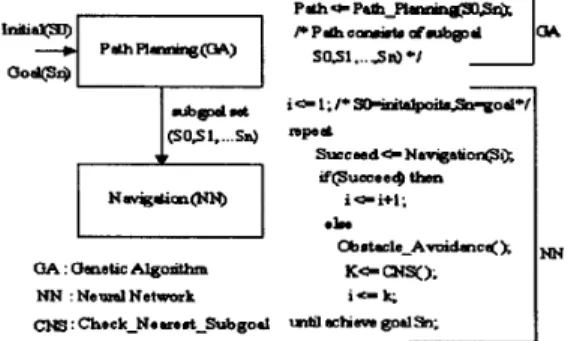
The overall architecture of the two-phase navigation system is shown in Figure 1. Given an arbitrary initial point and any goal point, the system will start by calling the 306

(2)

genetic path planner. The initial collision-free path, con- sisting of several subgoal points, is then passed t o the navigation module that controls the robot t o move along the planned path. If there is any unknown obstacle in the way while executing the task, the navigation controller will react to the environment based on its sensor readings in order to avoid collision. When the obstruction is cleared, the system will continue to achieve the task by moving t o the nearest subgoal point on the originally planned path.

Figure 1: Two-Phase Navigation System Architecture

3 Global

Genetic Path Planner

There are many path planning methods that can generate a collision-free path for a robot t o move from its initial position t o its goal position on a given map [7]. One of the earliest methods is visibility graph, which has been widely used for mobile robots [14]. The principle idea is t o construct a semi-free path composed of line segments connecting the initial point to the goal through vertices of obstacles. Constructing the visibility graph requires O(n3) time, where n is the total number of vertices of obstacles [9]. The standard A' algorithm, with the Eu- clidean distance as the heuristic evaluation function, can guarantee finding the shortest path if one exists. How- ever, finding the optimal path may be unnecessary if a robot has to modify its path in order to avoid collisions with unknown obstacles. Insteadiing of spending a lot of time finding the shortest path that will be changed later, it is a better idea t o find a reasonable path quickly in a dynamic environment.

Genetic algorithms are an effective parallel search technique [3], and it can be used to find a collision-free path on a visibility graph within a relatively short time. In addi-

tion, given more time, a genetic algorithm can refine the current solutions incrementally in search of the optimal solution. The proposed architecture uses a modified SGA (simple genetic algorithm) that can manipulate variable- length strings necessary t o represent robot paths in the search process.

3.1 Genetic representation

Given a map containing all known objects in the envi- ronment, the planner assigns a number t o each vertex of the obstacles, the initial point, and the goal point. A path consists of a sequence of vertices from the starting point t o the end point. Each chromosome corresponds t o a path represented by a sequence of numbers. Variable-length strings are used to represent chromosomes in order to deal with paths of arbitrary lengths. A population is then defined as a set of variable-length strings. For example, "pi : I 8 6 5 15" denotes a chromosome representing a path from point 1 to point 15 through vertices 8, 6, and 5. 3.2 Reproduction operators

Two reproduction operators, crossover and mutation, are used by the genetic planner.

Crossover Given two parent strings from the current population, crossover is achieved by choosing a crossover point (denoted by @) and then swapping the substrings from both parents about the chosen point. Since the lengths of any two parent strings may be different, the crossover point is chosen based on the shorter string. By swapping the substrings of numbers following the crossover point, two new strings are created. A number may appear more than once in a new string created this way, indicating a loop in the corresponding path. In this case, the redundant numbers are removed. For example, consider two parent strings A I and A2:

parent A I : I 8 6 @ 5 7 15

parent A2: I 4 3 @I 6 15

child C l : I 8 6 15

child C2 : I 4 3 5 7 15

Mutation Three mutation operators are defined:

r e p l a c e , add and d e l e t e . The replace operator updates a number with a new random number as defined in SGA. The add and delete operators are specially designed for this application. Add inserts the number corresponding to an arbitrary vertex into a randomly selected place; d e l e t e

removes a randomly selected number except the first and 307

(3)

last numbers. As a result, new individuals of variable length can be generated, The results of the mutation operators on a chromosome (the point at which mutations take place is indicated by *) are shown below:

Current: 1 8 6 f 5 7 15 Replace: 1 8 6 2 7 15 Add : 1 8 6 4 5 7 1 5 Delete : 1 8 6 7 15 3.3 Natural selection

The genetic planner uses a combination of the standard roulette wheel parent selection technique and the elitist strategy. The random selection technique dictates that an individual chromosome's chance of being selected is proportional to its fitness. On the other hand, the elitist strategy copies the fittest individual(s) into the new generation in order to avoid losing the best chromosome(s) of the old generation by accident.

3.4 Fitness function

There are two criteria for deciding the quality of a candi- date path: the percentage of free segments and the overall path length. Given two vertices vi and v , , the path segment between them is free if and only if the straight line ";vj does not intersect with any obstacles, and the path length is defined as the Euclidean distance between .y. and

v j . The Euclidean distance of a chromosome is the sum- mation over path length of every segment in the path.

Given a chromosome z in the population, its fitness evaluation function is defined as the weighted sum of these two criteria as follows:

where p ( z ) is the percentage of free segments in z, Pma2 is maxi p ( z i ) in the current population, d ( z ) is the Euclidean distance of the chromosome z, and Dma2 is max;d(zi) in the current population. Maximizing fitness therefore entails finding individuals with freest path and shortest path length. Tuning the relative weight of these two criteria plays an important role in finding a good quality path within a short time. At the beginning, the weight is set to be high in order to gather more feasible paths in the population. Once a free path has been found, the weight is decreased gradually so that the search will focus more on finding the shortest paths. The strategy is based on two observations. First, the path between two

vertices that are closest together is not always collision- free. Secondly, once a population contains enough free paths, future generations will continue to be mostly free. The process terminates when the relative error of two generations is below a threshold value. If the fitness of the resulting population is not satisfactory, i.e. a local max- imum, the system should increase the mutation rate and continue the process.

3.5 Tabling

In general, the cost of path planning is dominated by the cost of constructing the visibility graph, which requires O ( n 3 ) in a straightforward implementation [9]. Given the assumption that the world may change dynamically, the genetic planner is only interested in finding a good path rather than the optimal path. I t is therefore not necessary to construct the complete visibility graph in advance. In the proposed architecture, the visibility graph is generated incrementally at run time. The freeness and distance between any pair of vertices are recorded in two separate tables in order to reduce repeated computation.

3.6 Performance analysis

The performance of the genetic path planner (GA) was compared with that of the visibility graph using A* search method (VG). Two criteria were evaluated: the time to find a path and the distance of the resulting path. The results are shown in Table 1. Each col- umn of the table records the average performance of VG and GA over ten randomly generated maps, each with n numbers of obstacles. The experiment was repeated for n=10,12,14,16,18,20. In comparison with GA, the time required by GV grows rapidly as the number of obsta- cles increases, while the resulting distance is only slightly shorter than that of GA. As a result, GA can better cope with real-time requirements when the number of obstacles is large.

Table 1: Performance Comparison * Time is mearured in 0.01 second * Distance is measured in 0.1 inch

I 7L II

(4)

4 Local

NN Navigation System

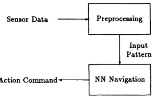
The local navigation module extracts features from raw sensor data. The processed data are then used as input patterns t o the neural network controller that selects an appropriate action for the robot t o perform in response to the current sensor readings. Figure 2 shows the overall operation cycle.

size of State is 43 with the infrared data being stored in StateCil t o StateC161 and the sonar data being stored in Statecl71 t o StateC321. Figure 4 illustrates the organization of the infrared and sonar regions on the robot. In addition, the current position coordinates 2, y can be

Sensor Data Preprocessing

Input Pattern

Action Command N N Navigation

L I

Figure 2: Operation cycle of the NN Controller

4.1 Robot hardware configuration

The Nomad 200 mobile robot used in our experiments is shown in Figure 3. It is composed of a circular omni- directional three-wheeled base and four sensory modules including infrared, ultrasonic, and tactile sensors, as well as a 2 D laser ranger.

-

Figure 3: The Nomad 200 mobile robot.

Figure 4: Sensor organization

found in State1341 and State1351, the steering angle of the robot is in Statec361; and the bumper state is in State1331 (State1331

#

0 indicates that the robot

has

collided with some objects.).

4.2 Preprocessing of sensor data

Due to the large amount of sensor data, it is necessary to preprocess the data in order t o minimize network topology as well as training time. The mobile robot uses infrared for short-range object detection and sonar for long-range object detection, which complement each other. Based on the circular arrangement of the sensors, obstacle avoidance and boundary tracing were implemented by segmenting the space around the robot into relevant sensory regions (see Figure 5 ) . The area in front of the robot was divided

In this research, only the first three modules were used. The infrared module consists of a ring of 16 sensors each of which returns a value from 0 t o 30 inches. The ul- trason module consists of a ring of 16 sensors each of which returns a value from 17 to 255 inches. The sensor data is returned through an array variable

-

State. The

Figure 5: Classification of sensor regions into tworegions: the danger zone and the safetysone. The zone dividing threshold of 20 inches was derived from the robot’s velocity and the minimumsonar range of Illinchea. 309

(5)

- -

It guarantees that a t least a subset of sensor data will be available before reaching an obstacle, thus decreasing the probability of any collision.

There are a total of 10 inputs to the neural network controller. Each input indicates a specific feature in the environment. Each input can be defined by a combination

+ o

Parallel_to-lcff_obstacle

fl

0

Parallel-to>&-obstacle of sonar, infrared and bumper data in the following way.

Frontsafehy_sonardetection: This input feature indicates if the front is clear based on sonar sensors. That is

,

Frontsafehyinfrareddetection: This input feature indicates that the front is clear based on infrared sensors. That is,

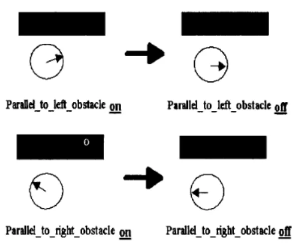
Figure 6: Parallel t o obstacle

moving into an obstacle, as is shown in Figure 6 . The input features can be defined as

O if mini=1,2,3,15,16(State[i])

<

20 or

I 2 =

[

mini=4,14(State[i])

5

6

( 1 otherwise

The second condition for the “0” case is necessary because the robot is not a point robot, and it may bump into obstacles on the side even if the front sensors do not detect

I s = { any obstacle. I 6 = 1 0 otherwise ’ 1 if min;=l2,l,l4(State[i])

<

20 and mini,g,lo,ll(State[i])

2

20 if mini=r,s,s(state[i])

<

20 and mini,.r,s,g(state[i])

2

20 0 otherwise 0 b s t a c l e i n r i g h t d a n g e r l o n e A w a y f r o m r i g h t a b s t acle

Obstacleinleftdangersone: Intuitively, the mobile Awayfromleft-obstacle: These two input features

robot _{are used to signal that the obstacle on the right (left)}

in Figure 7, After getting away from the obstacles, the

toward areas with fewer

When Obstacle are detected by the front we must _{side is}

no longer blocking the way. The situation is shown check whether they fall more within the left side or the

right side of the danger zone. We define two scores to estimate the distance to obstacle(s1 on the left and right

In addition, goal attraction can be taken into considera-

LJ

W

tion. If the goal is toward the right side of the robot, then increment R; otherwise increment L. The inputs are then

Away-from-right-obrtaclc Awry-from-le ft-obstacle

defined as:

0 i f R 2 L;

1 otherwise Figure 7: Away from obstacle

0 if L

>

R; system should check if the distance to goal has increased 1 otherwise since obstacle avoidance last started. If so, the robot should stroll along the obstacles until the distance to goal is shorter than or equal to the original distance. Input 7 references sonar 19, 20, 2 1 and infrared 6, 7, 8; input 8 references sonar 29, 30, 31 and infrared 10, 11, 12. Parallel-toright -obstacle

Parallel-toleft-obstacle: These two features describe if the robot is parallel to some obstacle on either side. Either input is on if the robot is in potential danger of

(6)

Bumper: This input, which references the tactile sensor data in S t a t e C331,

is

set to be on whenever the robot has bumped into any obstacles. Otherwise, it is off.

Direction: When the robot has rotated to the direction of the goal, this input becomes on. Otherwise, it remains Off.

4.3 Network topology

The local navigation controller was implemented as a

three-layer neural network with one hidden layer. The topology is shown in Figure 8. Based on the input defi- nitions in the previous section, there are 10 input nodes, 17 hidden nodes and 6 output nodes. Each node of the

vl.l

1 7 neurons

Figure 8: The topology of navigation controller output layer dictates a specific action for the robot to per- form. Multiple output nodes may be on at the same time. The six output actions of the navigation controller are explained below:

1. Orientdogoal:

Rotate to the direction of the goal. 2. Moveforward:

Move in the current direction for a fixed distance. 3. Movebackward:

Move opposite the current direction for a fixed dis- tance.

4. Turn-Left:

Rotate counter-clockwise for a fixed angle.

5. TurnRight:

6. Stop: Terminate all actions. Rotate clockwise for a fixed angle.

4.4 The training process

A set of 60 training examples were collected automatidly by operating the mobile robot in the simulator using a hand-coded collision avoidance program. The standard backpropagation method is used t o train the navigation controller. The learning algorithm from [12; 4; 81 was used: 8 E W ( t

+

1)

=

W ( t )

-

€-

+

a ( W ( t )

-

W ( t

-

1))

a w l

where W ( t

+

1) W ( t ) W ( t

-

1) E € : learning rate; a : momentum term. : weight at time t

+

1; : weight at time t; : weight at time

t

-

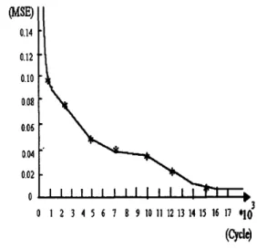
1; : sum of square error;

The learning rate and the momentum term were fixed in the entire training process. The number of hidden lay- ers and nodes were determined through a series of experiments. Once the topology was designed, the training process took approximately 12 hours on a

PC

386. The weights converged to a mean square error of less than 0.011 after about training 15000 cycles (60 patterns for each cycle). Figure 9 shows how the mean square error converged during the training process.

0.10 0.08 0.06 0.04 0.02 0 0 1 2 3 4 5 6 7 B 9 10 11 12 13 14 15 16 17

*I(

Figure 9: The learning curve in the training phase

(7)

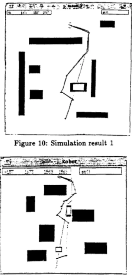
Figure 10: Simulation result 1

Figure 11: Simulation result 2

5 Simulation Results

The trained neural network waa tested on the simulator using randomly generated environments. Our experiments showed that given a n arbitrary map with unknown obet& cles, the robot can get to its destination successfully for about 90% of the time. The success rate can be improved if the clearance (as defined by the safety zone) on the side is reduced. Figures 10, 11 and 12 show the robot traces from several simulation runs. In these figures, the filled objects are assumed t o be known in advance and the outlined objects represent unknown obstacles. The thin line indicates the path generated by the genetic path planner and the thick line is the actual robot trajectory. In addition, the performance of the hand coded collision avoidance program and the neural network controller are compared.

As

shown in Figure 13, our system outper- formed the hand-coded program in most situations.

Figure 12: Simulation result 3

m

-i,-

Figure 13: Sample comparison of hand-coded (left) and neural networks (right) collision avoidance navigation.

(8)

6 Conclusion

[8] R. Lippmann, "An introduction t o computing with IEEE ASSP Magazine, 4:4-22, In this paper, we have presented an implemented naviga-

tion system that can effectively achieve its goal configurations in a partially known environment with unknown obstacles. The global path planner uses genetic algorithms t o search for a colliiion-free path on the visibility graph constructed among known obstacles. The local reactive navigator tracks the path while avoiding unknown obstacles using a neural network that maps run-time sensory information into the appropriate action(s). Our empirical data showed that the GA path planner can find a near- optimalfree path in less time than the standard A* search. The quality of the path is proportional to the amount of time available at the planning stage. The neural network controller reacts t o its sensor data with minimal amount of detouring from the planned path. It also outperforms the hand-coded collision avoidance program in terms of to learn, the two-phase system can successfully adapt to changes in the environment.

neural networks", 1987.

[9]

T.

Lorano-Pdrea and M.A. Wesley, "An algorithm for planning collision-free paths among polyhedral obstacles", Communications of the A

CM,

22( 10):560-570, 1979.

[lo]

y.

Mae&, M. Tanabe, M. Yuta, and T. T h i ,

Yoichuo Maeda, Minoru Tanabe, Morikasu Yuta, and Tomohuo Takagi, "Hierarchical control for au- tonomous mobile robots with behavior-decision fussy algorithm", Proc. IEEE int. Conf. Robotics and Au- tomation, pp. 117-122, 1992.

[ll] Maja J. Mataric, "Integration of representation into goal-driven behavior-based robots"

,

IEEE %ns. Au- tomatic Control, 8(3):304-312, 1992.

the resulting path length and time. Due to its ability J.L. McClelland and D.E. Rumelhart, parallel Dis- tributed Proc,essing, Reading, MIT Press, 1986. [13] S. Nagata, M. Sekiguchi, and K. Asakawa, "Mobile

Refer

en

c es robot control by a structured hierarchical neural net-

work", IEEE l'kans. Automatic Control, pp. 69-76, [l] Y. Davidor, "A Genetic algorithm Applied t o Robot 1990.

Trajectory Generation", PhD dissertation, Imperial College, London, 1989.

[14] N. J. Nibson, KA Mobile Automaton: An Application of Artificial Intelligence Techniques", Proceedings of the 1st International Joint Conference on Artificial Intelligence, pp.504-520, 1969.

[2] L. Davis, Handbook of Genetic Algorithms, Van NOS- trand Reinhold, Reading,

NY,

1991.

[3] D.E. Goldberg, Genetic Algorithms in Search, Op- timization, and Machine Leaming, Addison-Wesley, 1989.

[15] A. Sankaranarayanan and M. Vidyasagar, "A new path planning algorithm for moving a point object amidst unknown obstacles in a plane : A new algorithm and a general theory for algorithm devel- opment.", Proc. of 29th IEEE Conf. Robotios and Automation, pp. 1930-1936, 1990.

[4] D.R. Hush and B.G. Horne, "Progress in supervised neural networks: What's new since Lippmann?", IEEE Signal Processing Magazine, pp. 8-39, 1993. [5] S. Ishikwa, "A method of indoor mobile robot naviga-

tion by using fussy control", Proc. of IEEE Interna- tional Workshop on Intelligent Robots and Systems, pp. 1013-1018, Osaka, 1991.

[6] T. Kimoto, D. Masumoto,

H.

Yamakawa, and S. Nib

gata, "Hierarchical sensory information processing model with neural networks", Proc. of the 1993 IEEE International Conference on Robotics and Automa- tion, 1993.

[7]

J . 4 . Latombe, Robot Motion Planning, Kluwer Aca- demic Publishers, 1991.