A Unified Scheme for Modeling Software Reliability with Various Failure Detection and Fault Correction Rates

全文

(1)Int. Computer Symposium, Dec. 15-17, 2004, Taipei, Taiwan.. A Unified Scheme for Modeling Software Reliability with Various Failure Detection and Fault Correction Rates Jung-Hua Lo Department of Information Management Lan-Yang Institute of Technology, I-Lan, Taiwan losir@mail.fit.edu.tw number of remaining faults, and failure detection rate. Most of these models have focused on the failure detection process. Consideration of fault correction process in the existing models is limited. However, to achieve desired level of software quality, it is very important to apply powerful technologies for removing the errors in the fault correction process. In reality, the fault correction rate is a function of the complexity of program modules, the manpower, the skill of testing teams, the deadline for the release of the software, etc. Experiments have been performed based on real data set, and the results show that the proposed models obtain a better result in estimating the number of initial faults and also indicate a goodness-of-fit in terms of the mean-of-squares error criterion. This paper is organized as follows. In Section 2, the properties of the related models are reviewed. An integration model of failure detection and fault correction processes is proposed in Section 3. In Section 4, we show how some existing NHPP models are re-evaluated from the viewpoint of delayed correction process and make some observations between the delayed-time NHPP models and the integrated model. The experiments and results are presented in Section 5. Finally, the conclusions are made in Section 6.. Abstract -Many software reliability growth models (SRGMs) have been developed to estimate some useful measures such as the mean value function, number of remaining faults, and failure detection rate. Most of these models have focused on the failure detection process and not given equal priority to modeling the fault correction process. But, most latent software errors may remain uncorrected for a long time even after they are detected, which increases their impact. The remaining software faults are often one of the most unreliable reasons for software quality. Therefore, we develop a general framework of the modeling of the failure detection and fault correction processes. Furthermore, we also analyze the effect of applying the delay-time non-homogeneous poisson process (NHPP) models. Finally, numerical examples are shown to illustrate the results of the integration of the detection and correction process. Keywords: Software Reliability Growth Models (SRGMs), Non-Homogeneous Poisson Process (NHPP), Mean Value Function (MVF), Failure Detection Rate, Fault Correction Rate.. 1. Introduction Software reliability can be viewed as a powerful measure of quantifying software failures and is defined as the probability of failure-free software operation for a specified period of time in a specified environment [1]. Therefore, in order to achieve a desired level of quality, the reliability of a software system must be high. The fault-detection and faultcorrection are critical processes in attaining good software quality. During the software detection process, testing cases are run and ultimately failures are detected. After detection, the debugging team should analyze the failure, locate the fault and fix the fault [2-4]. That is, the fault correction process affects the reliability of a software product significantly and we should pay more attention to it. Recently, many SRGMs have been developed to estimate some useful measures such as the MVF,. 2. Some SRGMs Based on NHPP Let {N(t), t ≥ 0} denote a counting process representing the cumulative number of errors detected by time t, m(t) be the MVF of the expected number of faults detected in time (0, t), and λ (t ) denote the failure intensity at testing time t. That is, they satisfy the following: m(t) = E({N(t), t ≥ 0}), (1) , (2) λ (t ) = dm(t ) / dt m( t + ∆t ) − m( t) = d (t ) × [ a − m(t )]∆t , (3). λ (t ) = d (t ) × ( a − m( t)) , m ( t) = a. 914. + ( m (0 ) − a ) exp( − ∫0t d (u ) du ) .. (4) (5).

(2) Int. Computer Symposium, Dec. 15-17, 2004, Taipei, Taiwan.. where a is the expected number of errors to be eventually detected (i.e. m( ∞) = a ) and d(t) is the. 2.4. A general continuous NHPP model [8]. error detection rate per error at testing time t. Thus, an SRGM based on NHPP with MVF m(t) can be formulated as. Similar to the above discussion in the discrete case, we have the following theorem aimed on a general continuous NHPP model.. m (t ) n −m ( t) e , n = 0 , 1, 2 , ... (6) n!. Theorem 2: Let m( t + ∆t) be equal to the quasi-. P { N (t ) = n} =. In general, we can have different SRGMs based on NHPP using different MVFs.. arithmetic mean of m(t) and a with weights w( t + ∆t ). 2.1. Goel-Okumoto model [5]. We have m( t) = g −1 {g ( a) + [ g ( m(0)) − g (a)]e − B(t )} ,. and 1- w( t + ∆t ) ,and if. where g is a real-valued, strictly monotonic, and differentiable function, a is the expected number of initial faults, and B( t) = ∫ t b ( u ) du . □ 0. The most well-known SRGM based on NHPP is the model proposed by Goel and Okumoto. This model assumes that the error detection rate per error in the testing phase is constant. Thus, it is identical to take d(t) = b in Eq. (4) and the MVF is derived by. 2.5. A delayed-time NHPP model [7, 8]. m( t) = a(1− e −bt ), a > 0, b > 0 , where a is the expected number of errors to be eventually detected and b represents the error detection rate per error.. We know that the time to remove a fault depends on the complexity of the detected errors, the skills of the debugging team, the available manpower, and the software development environment [1, 9, 10]. Therefore, the time spent by the correction process is not negligible. Schneidewind [2, 11] first modeled the fault-correction process by using a delayed errordetection process and assumed that the errordetection process follows the NHPP and the rate of change of the MVF is exponentially decreasing. Furthermore, the fault-detection process in the Schneidewind model is isomorphic to the G-O model, except that the G-O model is viewed as a continuoustime process. Xie [2] extended the Schneidewind model to a continuous version by substituting a timedependent delay function for the constant delay in the Schneidewind model. Thus, we remove the impractical assumption that the fault-correction process is perfect and can thus establish a corresponding time-dependent delay function to fit the fault-correction process in our past research [7]. That is, the new MVF is m( t) = a(1 − e − bt eb ϕ (t ) ), a > 0, b > 0, (8). 2.2. Yamada s-shaped curve model [6] Yamada et al. assume that the error detection rate is a time-dependent function. That is, b 2t d(t) = , 1 + bt and,. lim 1 − w(t + ∆t) = b(t ) . ∆t → 0 ∆t. m( t) = a[1 − (1 + bt) e −bt ], a > 0, b > 0 .. 2.3. A general discrete NHPP model [7, 8] The two parameters, a and b play the same role as the a and d(t) in Eq. (4). Taking w = 1-b, we have m(i+1)=wm(i)+(1-w)a (7) This indicates that m(i+1) is equal to the weighted arithmetic mean of m(i) and a with weights w and 1 – w. More generally, the weighted arithmetic mean in Eq. (7) can be replaced by the weighted geometric, harmonic or quasi-arithmetic † means to derive other existing NHPP models [8]. Thus, we have the following theorem:. where a and b are the parameters in G-O model, ϕ (t ) is a delay-effect factor to represent the corresponding time-dependent lag in the correction process.. Theorem 1: Let g be a real-valued and strictly monotone function and m(i+1) be equal to the quasiarithmetic mean of m(i) and a with weights w(i+1) and 1–w(i+1), then m( i) = g −1{ui g ( m(0)) + (1 − ui ) g ( a)},. 3. An Integrated Model. i. where 0< w(i) <1, a > 0, ui = ∏w( j) for i ≥ 1 and u 0 = 1. j =1. □ †. The quasi-arithmetic mean z of x and y with weights w and 1-w is defined as g(x)=wg(x)+(1-w)g(y) where g is a realvalued and strictly monotone function.. 915. In the past, much research on software reliability models have concentrated on modeling and predicting failure occurrence and have not given equal priority to modeling the fault correction process [12]. However, most latent software errors may remain uncorrected for a long time even after they are detected, which increases their impact. The remaining software faults are often one of the most.

(3) Int. Computer Symposium, Dec. 15-17, 2004, Taipei, Taiwan. Thus, m( t) = e − D(t )[ ae D(t ) − a] = a(1 − e − D (t ) ) .. unreliable reasons for software quality. Therefore, we develop a general framework of the modeling of the failure detection and fault correction processes.. As for Eq.(10), we can multiply both sides with e C (t ) , d we have ( eC (t )mc (t )) = a∫0t c( s) eC (s ) (1 − e− D (s ) )ds . dt Finally, we have the result, mc ( t) = e − C (t ){∫0t ac( s )e C ( s ) (1 − e − D (s ) ) ds} . □. Assumptions 1. The error-detection process follows the NHPP. 2. The software system is subject to encountering the remaining faults in the system at random times. 3. All faults are independent and equally detectable. 4. The mean number of faults detected in the time interval (t, t+∆t) is proportional to the mean number of faults remaining in the system. The proportionality, λ (t ) , may generally be a time-. 3.2. Constant rate in these two processes Note that λ (t ) in Eq.(9) is generally a timedependent function and can be rewrite as m' (t ) λ (t ) = , a > 0. a − m(t ). dependent function [2]. 5. The mean number of faults corrected in the time interval (t, t+∆t) is proportional to the mean number of detected but not yet corrected faults remaining in the system. The proportionality, µ(t) , may also be. From the above equation, λ (t ) can be interpreted as the failure detection rate per remaining fault. In particular, solving the differential equation (9) with λ (t) = b under the initial condition m(0)=0 yields the. time-dependent [2]. 6. Each time a failure occurs, the fault is perfectly removed with no new faults being introduced.. following MVF: m( t) = a(1 − e − bt ), a > 0, b > 0 . Based on the above equation, the case is G-O model. Furthermore, µ(t) in Eq.(10) has a similar. 3.1. Description of the modeling. interpretation. That is,. Based on the above assumptions 1-6, we have the following differential equations for the MVF m(t) and mc (t) of failure detection and fault correction processes : dm( t) = λ ( t)( a − m(t )), a > 0, dt dmc ( t) = µ (t )[ m( t) − mc (t )]. dt To develop a framework of the modeling of these processes, we thus derive the following theorem.. mc ' ( t) . m( t) − mc (t ) By the above deduction, µ(t) is just the fault correction rate per detected but not corrected fault. Particularly, if λ (t ) and µ(t) equal b, the corresponding MVF is derived as follows: µ( t) =. Corollary 1: If the differential equations for the MVF m(t) and mc (t) of failure detection and fault correction processes is as follows: dm( t) = b(a − m(t )), a > 0, b > 0 dt dmc ( t) = b[ m(t ) − mc ( t)]. dt Therefore, we have m( t) = a[1 − e − bt ] ,. Theorem 3: If D (t ) = ∫ t λ ( s ) ds , C (t ) = ∫ t µ ( s ) ds , 0 0 and the differential equations for the MVF m(t) and mc (t) of failure detection and fault correction processes is as follows: dm( t) = λ (t )( a − m( t)), a > 0, (9) dt dmc ( t) = µ (t )[ m( t) − mc (t )]. (10) dt we have m( t) = a[1 − exp(− D( t))] , (11). mc ( t) = a[1 − (1 + bt) e − bt ] using the initial condition m(0)=mc (0)=0, i.e. no failure at the beginning. □. mc ( t) = e − C (t ){∫0t ac( s )e C ( s ) (1 − e − D (s ) ) ds} (12) where a is the expected number of initial faults, and the initial condition m(0)=mc (0)=0, i.e. no failure at the beginning. Proof: Solving the above differentiable eq.(9) by multiplying both sides with e D (t ) , we get d D( t ) d ( e m(t )) = a (e D(t ) ) dt dt. Corollary 2: If the differential equations for the MVF m(t) and mc (t) of failure detection and fault correction processes is as follows: dm( t) = λ (a − m(t )), a > 0, λ > 0 dt dmc ( t) = µ[m( t) − mc (t)]. dt we have, m( t) = a[1 − exp( −λ t)] ,. 916.

(4) Int. Computer Symposium, Dec. 15-17, 2004, Taipei, Taiwan. µ λ e −λ t − e − µt ] (13) λ −µ λ −µ where a is the expected number of initial faults, and the initial condition m(0) and mc (0) equal zero. □. 4.4. Comparisons approaches. m c (t ) = a[1 +. for. these. three. From the above derivation, we know that Yamada S-shaped curve can be interpreted from various points of view. In other words, by specifying the b 2t error detection rate per error, i.e. d(t) = in Eq. 1 + bt (5). Moreover, from the viewpoint of delayed-time correction phenomenon, we can choose a proper delay-effect factor, i.e. ϕ (t) = b1 ln(1 + bt) in Eq. (8).. 4. Comparisons and Observations Numerous stochastic models for software failure phenomenon have been developed to measure software reliability, and many of them are based on NHPP. In fact, these models are very useful to describe the software failure detection and correction processes with suitable failure occurrence rates. In this following, we discuss how several existing SRGMs based on NHPP mo dels can be comprehensively derived by applying some various factors. Specifically, we focus on the Yamada Sshaped curve model [6].. This factor is able to reflect the time lag in the correction process. Furthermore, if λ (t ) = µ (t ) = b in the integrated approach of Section 3, the S-shaped curve can be described. Thus, we make the following observations: Ÿ The classical NHPP MVF, is identical to the general delayed-time form of the MVF. Ÿ Many existing NHPP models for software reliability can be derived as special cases of this integrated framework of detection and correction processes.. 4.1. Error detection rate approach From Section 2 we know that we can have different SRGMs by using various d(t) in Eq. (5). For b 2t example, given d(t) = and m(0) = 0 in Eq. (5), 1 + bt we can get its corresponding MVF m(t) by the integration of d(t) as shown below: m( t) = a(1 − (1 + bt )e − bt ), a > 0, b > 0.. 5. Numberical Examples 5.1. Estimation and criteria for comparison. That is, a variation of the G-O model, known as the Yamada S-shape curve model [13], can be derived.. Without loss of generality, we discuss three kinds of approaches described in Section 3 to model the fault correction process. The first approach is about the delayed-time NHPP model, where ϕ (t ) is the. 4.2. Delay-time approach. Rayleigh function, i.e. ϕ (t ) = cte. Moreover, we can have different delay-time NHPP models by applying various delay-effect factors. Therefore, if ϕ (t) = b1 ln(1 + bt) , we can also get its. case discusses the general case of the proposed approach in Section 3 where the failure detection rate and fault correction rate are different constants, i.e. λ (t ) = λ , µ( t) = µ . Furthermore, the third case is. corresponding MVF by Eq. (8) as below: m( t) = a(1 − e − bt e bϕ (t ) ) = a(1 − (1 + bt)e − bt ), a > 0, b > 0.. the integrated model with equal value of rate, i.e. λ (t ) = µ (t ) = b . When the three case are applied to. This example reflects the fact that the S-shape model can be interpreted from various points of view. In other words, by specifying the error-detection rate per error or the delay-effect factor, we can formulate various models with a new MVF.. the equation (8)-(10) and it is solved with respect to MVF m(t) under the initial condition m(0)=0, we obtain the following equation, respectively:. − ( θt ) 2. . The second. − ( t )2. m1 (t ) = a (1 − e −bt exp(bcte θ )), (14) µ λ m 2 ( t) = a[1 + exp( − λt ) − exp( − µt)] (15) λ −µ λ −µ. 4.3. An integrated approach. m3 ( t) = a(1 − (1 + bt) e −bt ). (16) For illustration of the proposed NHPP models based on the above approach, we present an experiment on one real data set. Two most popular estimation techniques are the maximum likelihood estimation (MLE) and the least squares estimation (LSE) [1, 9, 10]. The maximum likelihood technique estimates parameters by solving a set of simultaneous equations. But the corresponding equations are usually complex and must be solved numerically.. Suppose both the failure detection rate per remaining fault, λ (t ) , and the fault correction rate per detected but not corrected fault, µ(t) , have the same value. That is, λ (t ) = µ (t ) = b. Therefore, we have the corresponding MVF as below: m( t) = a(1 − (1 + bt) e− bt ), a > 0, b > 0.. 917.

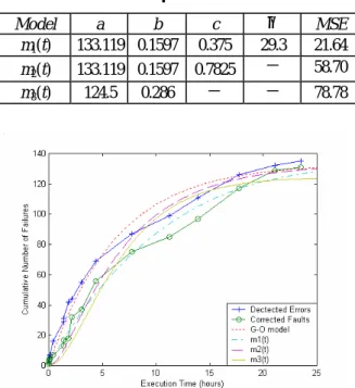
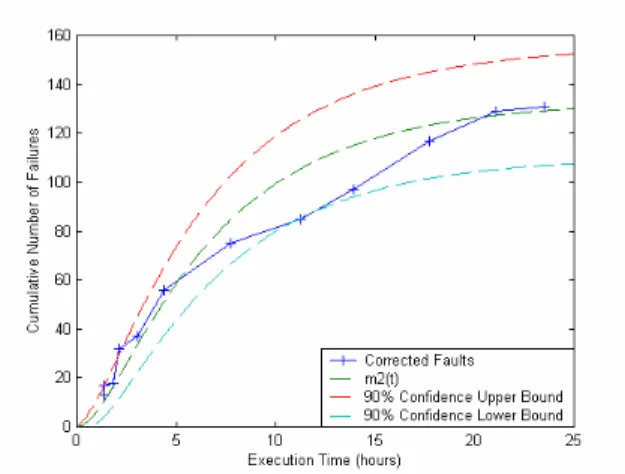
(5) Int. Computer Symposium, Dec. 15-17, 2004, Taipei, Taiwan.. Table 1. Estimated parameters for T1 data.. Furthermore, we use the method of least squares to minimize the sum of squares of the deviations between what we actually observe/get and what we expect. On the other hand, we adopt one evaluation criterion in the comparison of goodness-of-fit of the models.. Model m1(t). a b 133.119 0.1597. c 0.375. m2(t) m3(t). 133.119 0.1597 124.5 0.286. 0.7825 －. θ 29.3 －. MSE 21.64 58.70. －. 78.78. 5.2. Performance analysis The data set was the System T1 data of the Rome Air Development Center (RADC) reported by Musa [9, 13]. The system T1, developed by Bell Laboratories, was used for a real-time, command and control system. The number of object instructions was about 21,700 and it took 21 weeks to do the software test. The data set includes 136 observed failures, recorded in the execution time. First, parameters of models are evaluated and the corresponding MVFs are obtained. Second, all the selected models are compared with each other based on the objective criteria. Table 1 shows the estimated parameters of the proposed models described in Eq. (14)-Eq. (16) solved numerically by MLE and LSE. The lower the MSE a model is, the better they fit the observed data. Figure 1 depicts the observed curves and the fitted curves of the cumulative numbers of failures using the G-O, m1(t), m2(t), and m3(t) models , respectively. Figure 2 illustrates the difference between the intensity functions of MVF predicted by these models. Examples of the estimated MVF, m1(t), m2(t), and m3(t), and their 90% confidence limits are shown in Figure 3-Figure 5. We can see from Table 1, Figure 3 and Figure 4 that the delayed-time model and the integrated model fit the data well. Especially, the delayed-time model has the smallest value of MSE (21.64); therefore, we can conclude that the delayeffect factor model gives a better fit in this experiment. Furthermore, Figure 2 shows the estimated instantaneous fault correction rate of these models, in which we find that the integrated approach is a bellshaped-type curve. In reality, the fault correction rate is a function of the complexity of program modules, the manpower, the skill of testing teams, the deadline for the release of the software, etc. At the beginning of the software correction process, the programmers usually remove easy-to-correct errors in the programs . That is, the correction rate is increasing in such testing phase. As time goes, the team becomes acquainted with the software-testing environment, with better skills, techniques and tools. These improvements may speed up the testing activities [1, 9, 10]. As time passes further, it is relatively more difficult for the correcting team to correct more errors. That is, the rate that resulted from the correction process becomes smaller. This phenomenon just fits the increasing-then-decreasing scenario of the human learning process.. Figure 1. The MVFs for G-O, m 1(t), m 2(t), m 3(t).. Figure 2. The estimated intensity functions.. Figure 3. The 90% confidence limits of m 1(t). 918.

(6) Int. Computer Symposium, Dec. 15-17, 2004, Taipei, Taiwan.. References [1] [2]. [3]. Figure 4. The 90% confidence limits of m 2(t).. [4]. [5]. [6]. [7]. Figure 5. The 90% confidence limits of m 3(t). [8]. 6. Conclusions In this paper, we have constructed a SRGM based on an NHPP, which incorporates the failure detection and fault correction processes, and have discussed the methods of quantitative reliability assessment based on this new model. We also make some observations between the delay-time NHPP model and the integrated model. Several numerical cases based on real control system have been presented and the results show that the delayed-time model and the integrated model fit the data well.. [9]. [10]. [11]. Acknowledgement [12]. This research was supported by the National Science Council, Taiwan, ROC., under Grant NSC 932213-E-267-001.. [13]. 919. M. R. Lyu. Handbook of Software Reliability Engineering, McGraw-Hill, 1996. M. Xie and M. Zhao, "The Schneidewind software reliability model revisited," Proceedings of the 3th International Symposium on Software Reliability Engineering , pp. 184-192, May 1992. S. S. Gokhale, "Software Reliability analysis incorporating fault detection and debugging activities," Proceedings of the 9th International Symposium on Software Reliability Engineering , pp. 64-75, November 1992. M. Ohba, "Software Reliability Analysis Models,'' IBM J. Res. Develop, Vol. 28, No. 4, pp. 428-443, July 1984. L. Goel and K. Okumoto, "Time-dependent Error-detection Rate Model for Software Reliability and Other Performance Measures,'' IEEE Trans. on Reliability, Vol. R-28, pp. 206211, August 1979. S. Yamada, M. Ohba, and S. Osaki, "S-shaped Reliability Growth Modeling for Software error detection," IEEE Trans. on Reliability, vol. R-32, No. 5, pp. 475-478, December 1983. J. H. Lo and S. Y. Kuo, and C. Y. Huang, “ Reliability Modeling Incorporating Error Processes for Internet-Distributed Software,” IEEE Region 10 International Conference on Electrical and Electronic Technology (TENCON 2001), pp. 1-7, Aug. 2001, Cruise Ship, SuperStar Virgo. R. H. Huo, S. Y. Kuo, and Y. P. Chang, "On a Unified Theory of Some Nonhomogeneous Poisson Process Models for Software Reliability," Proceedings of International Conference on Software Engineering: Education & Practice, pp. 60-67, January 1998. J. D. Musa, A. Iannino, and K. Okumoto. Software Reliability, Measurement, Prediction and Application, McGraw-Hill,1987. J. D. Musa. Software Reliability Engineering: More Reliable Software, Faster Development and Testing, McGraw-Hill, 1998. N. F. Schneidewind, "Analysis of Error Processes in Computer Software," Sigplan Notices, Vol. 10, pp. 337-346, June 1975. N. F. Schneidewind, "Fault Correction Profiles," Proceedings of International Symposium on Software Reliability Engineering, pp. 60-67, 2003. J. D. Musa, Software Reliability Data, Report and Data Base Available from Data and Analysis Center for Software, Rome Air Development Center (RADC). Rome, NY. 292-296, May 1985..

(7)