A Study on the Bottleneck Power-Aware Many-to-One Routing Problem for Wireless Sensor Networks

全文

(1)A Study on the Bottleneck Power-Aware Many-to-One Routing Problem for Wireless Sensor Networks Pi-Rong Sheu Yu-Ting Li Hung-Yuan Tsai Chu-Yi Ho Department of Electrical Engineering, National Yunlin University of Science & Technology Touliu, Yunlin 640, Taiwan, R.O.C.. Abstract. [2], Energy Aware Routing [10], and MLDA & MLDR [6]. Most of the existing power-aware routing protocols are designed primarily to maximize the lifetime of WSNETs. (One of the common definitions of the network lifetime is the time period from the beginning of the network operation to when one of the nodes exhausts its battery power).To achieve the goal, the key mechanism adopted by many current power-aware routing protocols is either to evenly distribute packet-relaying loads to each sensor to prevent the battery power of any sensor from being overused [9] [12] or to minimize the total transmission power consumption of the entire WSNET [8] [14]. Let us use Figure 1 to illustrate the difference between the two strategies. In Figure 1(a), each node is supposed to possess the same battery power of 100. The number next to each link represents the power to be consumed when one data packet is delivered through the link. There are three source sensors ( vs1 , vs2 , and vs3 ) and one sink node vsink in the network. Every source sensor wants to send one data packet to the sink. Now, if we use the shortest path strategy, as shown in Figure 1(b), the network’s total transmission power consumption will be (5 + 5) + (3 + 5) + (5 + 5) = 28 and the network’s. Since the operations of sensors in a wireless sensor network mainly rely on battery power, power consumption becomes an important issue. To extend the network’s lifetime, many power-aware routing protocols have been designed to evenly distribute packet-relaying loads among nodes to prevent the overuse and abuse of battery power of any node. In this paper, we will consider the problem of searching for multiple routing paths between multiple source sensors and the single sink in a wireless sensor network such that the maximum of all the node’s power consumptions is as small as possible. We will first show such a problem to be NP-complete. Next, based on Dijkstra’s algorithm, an efficient heuristic algorithm is developed for the difficult problem. Computer simulations verify that the suboptimal solutions generated by our heuristic algorithm are very close to the optimal ones obtained by linear programming techniques. Keywords： NP-Complete, Power-Aware, Routing Algorithm, Sensor Network.. 1. Introduction. lifetime. A wireless sensor network (WSNET) is formed by a large number of tiny sensing devices (or called sensors) [8] [14]. A sensor in a WSNET can generate as well as forward data, which are gathered from every sensor’s vicinity and will be delivered to the single remote base station (or called the sink). Two sensors in such a network can communicate directly with each other through a single-hop routing path in the shared wireless media if their positions are close enough. Otherwise, they need a multi-hop routing path to finish their communications. In a multi-hop routing path, the data packets sent by a source sensor are relayed by several intermediate sensors before reaching the sink. WSNETs are useful in a broad range of environmental sensing applications such as vehicle tracking, seismic data, and so on. The research of WSNETs has attracted a lot of attention recently [8] [14]. In particular, since WSNETs are characterized by their limited battery-supplied power, extensive research efforts have been devoted to the design of power-aware routing protocols [8] [14]. At present, several efficient power-aware routing protocols have been developed, such as LEACH [5], Directed Diffusion. will. be. ⎢100 ⎥ ⎢100 ⎥ ⎢100 ⎥ ⎢100 ⎥ min{⎢ ⎥,⎢ ⎥,⎢ ⎥,⎢ ⎥} ⎣ 5 ⎦ ⎣ 3 ⎦ ⎣ 5 ⎦ ⎣ 15 ⎦. = min{20,33,20,6} = 6. If we use another strategy, as shown in Figure 1(c), the network’s total transmission power consumption will be (7 + 6) + (3 + 5) + (8 + 6) = 35 and the network’s ⎢ lifetime will be min{⎢. 100 ⎥ ⎢100 ⎥ ⎢100 ⎥ ⎢100 ⎥ ⎢100 ⎥ ⎢100 ⎥ ⎥ , ⎢ ⎥ , ⎢ ⎥ , ⎢ ⎥ , ⎢ ⎥ , ⎢ ⎥} ⎣ 7 ⎦⎣ 3 ⎦⎣ 8 ⎦⎣ 6 ⎦⎣ 5 ⎦⎣ 6 ⎦. = min{14,33,12,16,20,16} = 12 . In the two situations, it is easy to observe that a smaller total transmission power does not imply a longer network lifetime, exemplified by the first strategy. On the other hand, we discover that when the power consumptions of nodes even out, the associated network’s lifetime will be longer, as the later strategy shows. In this paper, we will take the approach of leveling each node’s power consumptions as a starting point. In WSNETs, the basic operation is the periodic gathering and transmission of sensed data packets to the sink for further processing [8] [14]. To be more specific, during a period of time (called a round), the sink first broadcasts a query for its interested data, then the sensors which posses the appropriate data (called the source sensors) deliver their data packets to the sink. Obviously, it is possible that a lot of. 1.

(2) source sensors want to communicate with the single sink simultaneously. In this paper, we will consider the problem that given multiple source sensors and the single sink in a WSNET, find a routing path between each source sensor and the single sink such that the maximum of all the node’s power consumption is as small as possible, namely, the power consumption of each node is as even as possible. Undoubtedly, the resulted lifetime of network is extended. We will name the problem as the bottleneck power-aware many-to-one routing (BPAMOR) problem. In this paper, we will first show the BPAMOR problem to be NP-complete. Then, based on Dijkstra’s algorithm, an efficient heuristic algorithm with low time complexity is developed for the difficult BPAMOR problem. Finally, by computer simulations, we verify that the suboptimal solutions generated by our heuristic algorithm are very close to the optimal ones obtained by linear programming techniques.. 7. vs1. 5. 3 6. In this section, we will introduce our some assumptions, notations, and definitions. A formal definition of our problem in terms of these notations and definitions will also been stated. In the following, the term “node” is synonymous with the term “sensor” and the term “link” is synonymous with the term “communication channel”. Assumptions The following states some important assumptions used in our research. (1) We assume that the wireless sensor network’s topology would not change, i.e. no sensor gets move [1] [7] [13]. (2) We only consider the transmission power and ignore the reception power [3]. (3) We assume that the required transmission power to establish a communication channel between any two sensors x and y is the same. In other words, c(< v x , v y >) = c(< v y , v x > ) , where c(< vx , vy >) and c(< vy , vx >) denote the minimal transmission power required by sensors x and y to establish < vx , v y > communication channels and < v y , v x > , respectively [3]. (4) We assume that when a data packet passes through a link, the transmission power consumption associated with the link can be an arbitrary value, i.e., can be independent of the Euclidean length of link [1] [3]. Traffic Model and Data Aggregation In the following, we will define a round as a period of time in which the sink first broadcasts a queue for its interested data, then the source sensors, which posses the related data, deliver their data packets to the sink. We assume that during each round, each source sensor generates one data packets to be transmitted to the sink. Data aggregation has been recognized as a useful routing paradigm in WSNETs [14]. The main idea is to combine data packets from different sensors to eliminate redundant messages and to reduce the number of transmissions such that the total transmission power of network is saved. One of the simplistic data aggregations is that an intermediate sensor always aggregates multiple incoming data packets into a single outgoing data packet. In the. 6. 5. v2. vsink 6. 5. 8. vs3. 2. The Definition of our BPAMOR Problem. v1. 5. vs2. The rest of the paper is organized as follows. In Section 2, a formal definition of the BPAMOR problem is given. In Section 3, the BPAMOR problem is shown to be NP-complete. In Section 4, an efficient heuristic algorithm for the BPAMOR problem is proposed. In Section 5, the performance of our heuristic algorithm is evaluated through simulations and compared to the optimal solutions. Lastly, Section 6 concludes the whole research.. v3. (a) 7. vs1. v1. 5. 5. 6. α (v2 ) = 15 3. vs2 6. vsink 6. 5. 8. vs3. 5. v2. v3. (b) 7. vs1. v1. 5. 5. 3. vs2 6. 6. 5. v2 5. 5. vsink 6. α (vs ) = 8 3. vs3. 8. v3 (c). Figure 1: An example to illustrate the BPAMOR problem.. 2.

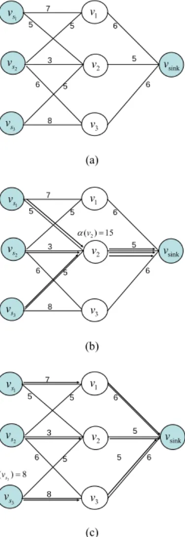
(3) 3. The Complexity of our BPAMOR Problem. following, for simplicity, we will deal with our BPAMOR problem without data aggregation. In fact, as discussed in [6], data aggregation is not applicable in all sensing environments. Problem Formulation We represent a WSNET by a weighted graph G = (V, E), where V denotes the set of sensors and the sink, and E denotes the set of communication links connecting the sensors or the sink. For E, we define a t r a n s m i s s i o n p o w e r c o n s u m p t i o n fu n c t i o n β : → R+ that assigns a nonnegative weight to each link in the network. The value β (i, j) associated with link (v i , v j ) ∈ E represents the transmission power that one data packet will consume on that link. For E, we define a data packet flow function f : E → I + . The value f (vi , v j ) denotes the number of data packets passing through link (vi , v j ) . For V, we define a node power c o n s u m p t i o n f u n c t i o n α :V → R + . Thus, α (vi ) = ∑ f (vi , vj ) × β (vi , v j ) represents the. In this section, we will show that our BPAMOR problem is NP-complete. To prove our BPAMOR problem to be NP-complete, first let us restate it in its decision version as follows: given a weighted graph G=(V,E), q source sensors vsi and the sink vsink , vsi , vsink ∈ V , a transmission power consumption + function β : E → R , a constant c p , find a set of q routing paths such that the maximum of node’s transmission power consumption in G is less than or equal to c p , i.e., max {α ( vi )} ≤ c p . vi ∈G. For simplicity, in what follows, we will not distinguish the decision version and the optimal version of the BPAMOR problem when no ambiguity arises. Next, let us introduce the 3-Dimensional Matching (3DM) problem [4]. Instance: A set M ⊆ W × X × Y , where W, X, and Y are disjoint sets having the same number q of elements. Question: Does M contain a matching, that is, a subset M ′ ⊆ M such that M ′ = q and no two elements of M ′ agree in any coordinate? This problem was shown to be NP-complete by Karp [4]. Now, we will use it to prove the following theorem. Theorem 1. The BPAMOR problem is NP-complete. Proof. First, the BPAMOR problem can be easily seen to be in the class NP. We next transform the 3DM problem to the BPAMOR problem in polynomial time. Let the sets W, X, Y, with W = X = Y = q , and M ⊆ W × X × Y be an arbitrary instance of 3DM. Let the elements of t h e s e s e t s b e d e n o t e d b y. (vi ,v j )∈E. total ransmission power that node vi will consume during a round. Under the BPAMOR problem we are considering, q routing paths originating from q source sensors vsi ∈ V in the WSNET have to be connected to the sink vsink ∈ V . Our target is to find the q routing paths such that the maximum of all the node’s transmission power consumptions in G is minimized. Based on these notations and definitions, we can now formally describe the BPAMOR problem in our paper: given a weighted graph G=(V,E), q source sensors vsi and the sink vsink , vsi , vsink ∈ V , a transmission power consumption function β : E → R + , find a set of q routing paths such that the maximum of all the node’s transmission power consumptions in G is minimized, i.e., max α ( vi ) is minimized. vi ∈G. {. W ={w1, w2, , wq} , X ={ x1, x2, , xq} ,Y ={ y1, y2, , yq}. }. and M = {m1 , m 2 , , m k } , where k = M . We construct an instance of the BPAMOR problem as follows: For each element wi of W, the corresponding weighted graph G = (V, E) has a source sensor v wi (1 ≤ i ≤ q). Similarly, for each xi and yi , G has sensors v xi and v yi , respectively. In addition, the sink node vsink is put into G. Thus, V = { vw1 , vw2 ,… , vwq } ∪ { vx1 , vx2 ,… , vxq } ∪ { v y1 , v y2 ,… , v yq } ∪ { vsink }. If ( wi , x j , y k ) ∈ M, then there exist one edge < vwi , v x j > between nodes v wi and v x j , and one edge < v x j , v yk > between nodes v x j and v yk . Furthermore, we connect each node v yk to the sink vsink . Thus, the edge set E = { < vwi , v x j > : if ( wi , x j , yk ) ∈ M }∪{ < v x j , v yk > : if ( wi , x j , yk ) ∈ M }∪{ < v yk , vsink > ：k =1, 2,…, q }. Each sensor node vi is assumed to have an amount α (vi ) = 1 of residual power capacity. All the edges have a transmission power consumption of 1 when. As an illustration of the above definitions and notations, let us consider the example shown in Figure 1. In Figure 1(a), let sensors vs1 , vs2 , and vs3 be the source sensors and vsink be the sink, respectively. The number next to a link represents the transmission power consumption of the link. If we use the shortest path strategy, we can see the result shown in Figure 1(b), and the node with maximal transmission power is v2 and the value is 15. If we use some strategies instead of the shortest path strategy, as shown in Figure 1(c), we can see that the node with maximal transmission power is vs3 and the value is 8. Therefore, we aim at designing efficient routing algorithms to minimize the maximum of all the node’s transmission power consumptions. Basically, this implies a longer network lifetime can be obtained.. 3.

(4) one data packet traverses it. Finally, let c p = 1 . The constructed G is illustrated in Figure 2. It is easy to see that this transformation can be finished in polynomial time. vw. 1 1 1. . . .. 1. 1. 2. 1. 1. 1. vx. vy. 2. 1 vw. vy. 1. 1 vw. 1. vx. 1. 1 1. 1. vw. 1. 3. 1 1. vwq. 1 vxq. vsink. . . .. In this section, we will propose a heuristic algorithm for the BPAMOR problem. This algorithm is based on the shortest-path concept, and we call it the BPAMOR algorithm. The basic idea of our BPAMOR algorithm is as follows: we improve the shortest-path concept by attempting to adjust each routing paths to reduce the maximum of node’s transmission power consumption. To be more specific, we firstly find a set of shortest paths from each source sensor to the sink by using Dijkstra’s algorithm. Then we modify each routing path by removing the sensor node with maximal transmission power consumption in the network if the required condition is matched. Figure 3 shows the pseudocode of our BPAMOR algorithm. In line 2, A is the set of source sensors and the. 1. 1. vy. q-1. 1. 1. vy. . . .. vx. q-1. 4. An Efficient Heuristic Algorithm for the BPAMOR Problem. 1. 3. . . .. 1. 2. 1 vx. 3. proof of NP-completeness. ▓ When a problem is proved to be NP-complete, the follow-up quest will be to search for various heuristic algorithms and evaluate them by computer simulations. In the next section, we will design an efficient heuristic algorithm for our BPAMOR problem.. 1. q-1. 1 1. cp = 1. vyq. Figure 2: An illustration of Theorem 1. We next show that a feasible solution for the BPAMOR problem exists in G if and only if the set M contain a matching M ′ . First, suppose M contain a matching, that is, a subset M ′ ⊆ M such that M ′ = q and no two elements of M ′ agree in any coordinate. If w i′ , x ′j , y k′ ∈ M ′ , then we let vwi′ , vx′j , v yk′ , vsink be a routing path in G for source sensor vwi′ . Since M ′ = q , there are q routing paths each of which is for a different source sensor vwi . Since no two elements of M ′ agree in any coordinate, these routing paths are pairwise node-disjoint except their common sink node. Because they are pairwise node-disjoint, any link (vi , v j ) belongs to at most one of these q paths. Therefore, for each link (vi , v j ) ∈ E , f (vi , v j ) ≤ 1 . Similarly, any node vi belongs to at most one of t h e s e q p a t h s . S o , f o r a n y vi ∈V , ∑ f (vi , v j ) ≤ 1 . Then, for any vi ∈V , we have. (. (. ). ( vi , v j )∈E. α (vi ) =. ∑. ( vi , v j )∈E. β (i, j ) × f (vi , v j ) =. ). ∑. ( vi , v j )∈E. sink. max α denotes the maximum of node’s transmission power consumption in the network. Initially, we set the value of max α , α (vi ) , and α '(vi ) to be zero, where α (vi ) is the transmission power consumption of each sensor vi and α '(vi ) is its temporary value. Line 4 to line 6 are to find the shortest path ri from each source sensor vsi to the sink by using Dijkstra’s algorithm. Line 7 to line 9 compute the transmission power consumption α (vi ) for each node vi . Line 10 and line 11 select the node vz with maximal transmission power consumption in the network and set max α to be the maximum value. Line 12 to line 30 are the process of adjusting each routing path. During the process of adjustment, we first select the sensor node vz (here we set v y = vz ), which has the maximal transmission power consumption, and remove it form the network temporarily. Next we check whether this sensor node vz is on the routing path of. 1× f (vi , v j ) ≤ 1 . As a. result max{α (vi )} ≤ 1 = c p . Thus, these q routing vi ∈V paths form a set of feasible routing paths for the corresponding general BPAMOR problem in G . Next, suppose we have a solution for the general BPAMOR problem in the weighted graph G. Let P1 , P2 , , Pq be one of the possible solutions in G . Because max{α (vi )} ≤ 1 = c p , α ( vi ) ≤ 1 for each. (vsi , vsink ) or not. If the removed sensor node vz is on the routing path of (vsi , vsink ) , we will re-find ' another routing path ri from vsi to vsink in G'.. vi ∈V. node vi . Furthermore, each link has a transmission power consumption of 1, and each node vi belongs to at most one routing path Pl (otherwise, α (vi ) > 1 ). Thus routing paths P1 , P2 , , Pq are pairwise node-disjoint except their common sink node. Let and Pt = ( v wt , v xt , v yt , vsink ) , Pt ∈ ( P1 , P2 , , Pq ) i j k then ( w t , x t , y t ) ∈ M ′ . Clearly M ′ = q and no two elements of M ′ agree in any coordinate. Thus, M ′ is a matching and M ′ ⊆ M. This completes our i. j. The checking operations are shown from line 15 to line 17. After finishing the checking, from line 18 to line 22, we will re-computer the transmission power consumption α '(vi ) for each sensor node vi . Line 25 compares the present maximum of the transmission power consumption α (vz ' ) with the. k. 4.

(5) Input: G = ( V , E ), a residual power capacity function α : V → R+ , a transmission power consumption function β : E → R + , q source sensors vsi and the sink Output:. previous one. 3. 4. 5.. ri by the new routing path ri ' and replace the α (vi ) by α '(vi ) ; Otherwise, nothing to do. After. path. vsink , v si , vsink ∈ V. max α is the maximum of node’s. finishing the checking process for each routing path. ri. with maximal transmission power consumption in the present status. All the above steps are repeated until the sensor node v y is equal to the new sensor node vz . Because as the new sensor node vz is equal to the original sensor node v y , nothing will happen in the following adaptation loops. Finally, we output the transmission power consumption α (vi ) of each sensor node vi and each routing path ri , where i = 1, 2,..., q . Example We will explain the operation of our BPAMOR algorithm by using Figure 4. In Figure 4(a), let nodes. with the smallest. total transmission power between. 6. 7. 8.. ri of (vsi , vsink ) , we search a new sensor node vz. netwrok ri , i ∈1, 2,..., q is the routing path for each source sensor vsi respectively. begin A = {(vs1 , vsink )(vs2 , vsink ),......, (vsq , vsink )} ; maxα = 0 ; for each vi ∈ V do { α (vi ) = α `(vi ) = 0 ;} end of for loop for each (vsi , vsink ) ∈ A do find the routing path. vsink by Dijkstra`s algorithm;. vsi. If the present one is smaller. than the previous one, we will replace the old routing. transmission power consumption in the. 1. 2.. α (v z ) .. and. 9.. end of for loop for each ri do for each v j ∈ V do {if (v j , vk ) ∈ ri then α ( v j ) = α ( v j ) + β ( v j , v k ) ;} end of for loop end of for loop. 10.. find the node v z whose. one data packet bypasses this link. Firstly, we execute. α (vz ) = max{α (vi )} ; v ∈V maxα = α (v z ) ; G ' = G ;. the Dijkstra’s algorithm from each source sensor to. 11. 12. 13. 14. 15. 16. 17.. 18. 19. 20. 21. 22. 23. 24. 25. 26. 27. 28.. 29. 30. 31. 32.. vs1 , vs2 , and vs3 be the source sensor nodes and nodes vsink is the sink node. The number next to each link represents the power to be consumed when. the sink to find its shortest path, as shown in Figure 4. i. do. (b). From Figure 4 (b), we can notice that the node. G ' = G '− vz ; y = z ;. for each (vsi , vsink ) ∈ A do if ( ri includes v z ) { find the routing path ri ' in G ` with the smallest total transmission power between vsi and vsink by Dijkstra`s algorithm; for each v j ∈ V do α '( v j ) = α ( v j ) ; if ( v j , v k ` ) ∈ ri ' then α '( v j ) = α '( v j ) + β ( v j , v k ' ) ; if ( v j , v k ) ∈ ri then α '( v j ) = α '( v j ) − β ( vi , v k ) ; end of for loop find the node vz ' whose α (vz ' ) = max{α '(vi )} ; v ∈V max'α =i α (vz ' ) ; if (max'α < maxα ) { ri = ri ' ; α (vi ) = α '(vi ) }end if } end if. with maximal transmission power consumption is. v2 and we set vz = v2 (here we also set v y = vz ). Next, we will remove the vz from the network temporarily and do the process of adjustment. Because the sensor node vz is on the routing path. r1 , we have to modify the routing path r1 . The new ' routing path r1 decreases the maximum of node’s transmission power consumption in the network, therefore we replace the routing path r1 by the new. r1' which is shown in Figure 4(c). The processes of modification for routing path r2 and routing path r3 will follow the same principle, routing path. which are shown in Figure 4(d) and Figure 4(e). From Figure 4(d), we notice that the maximum of node’s transmission power consumption increases due to the replacement of new routing path. end of for loop find the node v z whose. will use the old routing path r2 instead of new. α (v z ) = max{α (vi )} ; maxα = α (v z ) ;. while( yvi ∈≠V z ) output α , ri , i end of the algorithm. r2' , we. routing path. = 1, 2,..., q ;. r2' . The modification of r3 is similar. with r1 . After the process of modification, we can get a new sensor node vz with the maximal. Figure 3: The pseudocode of our BPAMOR algorithm.. transmission power consumption in the network. In 5.

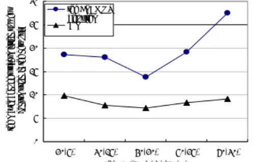
(6) simulations to evaluate the performance of our ILP formula [11] and our BPAMOR algorithm in terms of maximal node’s transmission power in the network and the execution time. Our computer simulations will be divided into three different simulation environments. In each simulation environment, we will observe the impact of one of the three parameters: the number of total links, the size of WSNET, and the structure of WSNET, on performance of our BPAMOR algorithm. In our first simulation environment, the total number of links will be varied and its influences will be observed. The environments in our first simulation are set as follows: the WSNET consists of 50 sensor nodes located in a 100 × 100 m2 area randomly. The transmission power consumption of each links is set from 1 to 20. The number of source sensors is set to 20. We will vary the total number of link from 10×n, 15×n, 20×n, to 24×n (where n is the total number of sensor nodes and 24×n means that the network is a complete graph). Notice that we neglect the 5×n because the execution time of ILP is too long (at least 3600 seconds each experiment). From Figure 5(a), we see that the maximal node’s transmission power consumption is decreasing with the increasing of the total number of links. This is because the more links exist in the network, the more routing path can be used for different source sensors. Figure 5(b) shows the execution times. The result of Figure 5 reveals that although ILP can get the optimal solution, the long execution time is its disadvantage.. Figure 4(f), because the new sensor node vz ( = vs3 ). is not equal to v y ( = vs2 ), we will continue our line. 12 to line 30 loop and reset the node v y . At this time, the node v2 has been removed temporarily last round, we can’t do any modification in this round, and therefore end our algorithm. From Figure 4(f), the node with maximal transmission power consumption is vs3 and the value max α is 8. Recall that, if we use the Dijkstra’s algorithm directly, the result is shown in Figure 4(b), and the node with maximal transmission power consumption is v2 and. maxα is 15.. the value 7. vs1. v1. 5. 5. 3. vs2 6. 7. vs1. 6. 5. 6 vz (v y ). 5. v2. v1. r1. 5. vsink. 3. v s2. 6. 5. 5. v2. r2 6. vsink 6. 5. r3 v3. 8. vs3. v3. (a). r1'. vs1. 7. (b). v1. 5. 5. r1. 6. r vsink. vy. 3. v s2 6. r3. 5. v2. r2. 6. 5. 6. 5. ' 2. 5. v2. r2. v1. 5. vy. 3. vs 2. r1 = r71'. vs1. 6. vsink. 25. 6. 5. the maximal node's ttransmission power consumption in the netwrok. 8. vs3. r3 8. vs3. 8. vs3. v3. v3. (c). (d). the BPAMOR algorithm ILP. 20 15 10 5 0. r1'. v1. 5. 5. vs1. 6. r1 = r1'. 10×n 7. v1. 5. 5. 3. vs2. v2. r2 6. vsink. 3. vs2. 6. 5. r3 vs3. vy. 5. v2. r2 6. 5. vsink. v3. ' 3. r. vs3. transmission power consumption in the network. 6. 5. 1800 r3 = r3' 8. maxα = α(vs3 ) = 8. (e). 24×n. (a) The effect of the total number of links on the maximal node’s. new vz. 8. 15×n 20×n total number of links. 6. vy. the BPAMOR algorithm ILP. 1600. v3. 1400 execution times (s). vs1. 7. (f). 1200 1000 800 600 400. Figure 4: An illustration of our BPAMOR. 200 0. algorithm.. 10×n. 5. Computer Simulations. 15×n 20×n total number of links. 24×n. (b) The effect of the total number of links on execution times. Figure 5：The first computer simulations.. In this section, we will conduct computer 6.

(7) the total number of sensor nodes. We observe that the performance of our BPAMOR algorithm keep static with the different structures of WSNET in Figure 7(a). That is, our BPAMOR can get a stable effect in any structure of WSNET. Figure 7(b) is the execution times.. In our second simulation environment, the total number of nodes will be varied and its influences will be observed. The environments in our second simulation are set as follows: the WSNET consists of n sensor nodes located in a 100 × 100 m2 area randomly. The transmission power consumption of each link is set from 1 to 20. The number of source sensors is set to 20. The total number of links is set N × ( N − 1) / 4 , where n is the total number of sensor nodes. We will vary the total number of sensor nodes from 30, 40, 50, 60, to 70. From Figure 6(a), we see that the maximal node’s transmission power consumption is decreasing with the increasing of the total number of sensor nodes. The impact of total number of sensor nodes is similar with that of total number of links. Figure 6(b) shows the execution times. We find that ILP needs more execution time to obtain the better performance.. 16. the maximal node's transmission power consumption in the network. the BPAMOR algorithm ILP. 20 15 10 5 0 20(5). 30(15). 40(20). 50(25). 60(30). the structure of network. (a) The effect of the structure of network on the maximal node’s transmission power consumption in the network. the BPAMOR algorithm ILP. 18. 25. 3500 3000. the BPAMOR algorithm ILP. 2500. execution times (s). the maximal node's transmission power consumption in the network. 20. 30. 14 12. 2000. 10. 1500. 8. 1000. 6. 500. 4. 0. 2. 20(5). 0 30. 40. 50 60 total number of nodes. 30(15). 40(20). 50(25). 60(30). the structure of network. 70. (b) The effect of the structure of network on execution times (a) The effect of the size of network on the maximal node’s. Figure 7：The third computer simulations.. transmission power consumption in the network. 6. Conclusions 1600 the BPAMOR algorithm ILP. 1400 execution times (s). 1200. In this paper, we have discussed the BPAMOR problem. We have shown the BPAMOR problem to be NP-complete. Based on Dijkstra’s algorithm, an efficient heuristic algorithm with low time complexity has been proposed to solve the difficult BPAMOR problem. Finally, by computer simulations, we have verified that the suboptimal solutions generated by our heuristic algorithm are very close to the optimal ones found by an optimal ILP program.. 1000 800 600 400 200 0 30. 40. 50 60 total number of nodes. 70. Acknowledgements. (b) The effect of the size of network on execution times. Figure 6：The second computer simulations.. This work was supported by the National Science Council of the Republic of China under Grant # NSC 93-2213-E-224-023. In our third simulation environment, the structure of WSNET will be varied and its influences will be observed. We will change the structure from 20(10), 30(15), 40(20), 50(25), to 60(30) (where 20(10) means there are 20 sensor nodes and 10 source sensors in the WSNET). The transmission power consumption of each link is set from 1 to 20. The total number of links is set N × ( N − 1) / 4 , where n is. References [1] M. Cagalj, J. P. Hubaux, and C. Enz, "Minimum-Energy Broadcast in All-Wireless Networks: NP-Completeness and Distribution Issues," Proceedings of the Eighth ACM 7.

(8) International Conference on Mobile Computing and Networking (Mobicom 2002), Sep. 2002. [2] I. Chalermek, G. Ramesh, E. Deborah, and H. John, “Directed Diffusion for Wireless Sensor Networking,” IEEE/ACM Transactions on Networking, vol. 11, no. 1, Feb. 2003. [3] W. T. Chen and N. F. Huang, "The Strongly Connecting Problem on Multihop Packet Radio Networks," IEEE Transactions on Communications, vol. 37, no. 3, pp. 293-295, Mar. 1989. [4] M. R. Garey and D. S. Johnson, Computers and Intractability: a Guide to the Theory of NP-Completeness, San Francisco: W. H. Freeman & Company, Publishers, 1979. [5] W. R. Heizelman, A. Chandrakasan, and H. Balakrishnan, “Energy-Efficient Communication Protocol for Wireless Micro Sensor Networks,” IEEE Proceedings of the Hawaii International Conference on System Sciences, pp. 1-10, Jan. 2000. [6] K. Kalpakis, K. Dasgupta, and P. Namjoshi, “Maximum Lifetime Data Gathering and Aggregation in Wireless Sensor Networks,” Proceedings of the 2002 IEEE International Conference on Networking ,Atlanta, Georgia, Aug. 2002. [7] A. Misra and S. Banerjee, "MRPC: Maximizing Network Lifetime for Reliable Routing in Wireless Environments," IEEE Wireless Communications and Networking Conference, vol. 2, pp. 800-806, Mar. 2002.. [8] C. S. R. Murthy and B. S. Manoj, Ad Hoc Wireless Networks: Architectures and Protocols, Prentice Hall, 2004. [9] C. E. Perkins, Ad Hoc Networking, MA: Addison-Wesley, 2001. [10] R. C. Shan and H. M. Rabaey, “Energy Aware Routing for Low Energy Ad Hoc Sensor Networks,” IEEE Wireless Communications and Networking Conference, 2002. [11] P. R. Sheu, Y. T. Li, H. Y. Tsai, and C. Y. Ho, "A Study on the Bottleneck Power-Aware Many-to-One Routing Problem for Wireless Sensor Networks," Technical Report, Department of Electrical Engineering, National Yunlin University of Science & Technology, Taiwan, R.O.C., 2005. [12] C. K. Toh, “Maximum Battery Life Routing to Support Ubiquitous Mobile Computing in Wireless Ad Hoc Networks,” IEEE Communications Magazine, vol. 39, pp. 138-147, Jun. 2001. [13] J. E. Wieselthier, G. D. Nguyen, and A. Ephremides, "On the Construction of Energy-Efficient Broadcast and Multicast Trees in Wireless Network,” Proceedings of the 19th IEEE INFOCOM, pp. 585-594, 2000. [14] F. Zhao and L. Guibas, Wireless Sensor Networks: an Information Processing Approach, Boston: Elsevier-Morgan Kaufmann, 2004.. 8.

(9)