Breast cancer classification and biomarker discovery from microarray data using silhouette statistics and genetic algorithms

Breast cancer classification and biomarker discovery from microarray data using

silhouette statistics and genetic algorithms

Tsun-Chen Lin

Dahan Institute of Technology

lintsunc@ms01.dahan.edu.tw

Yu-Wu Wang

Dahan Institute of Technology

s9389013@ms02.dahan.edu.tw

Ru-Sheng Liu

Yuan Ze University

csrobinl@saturn.yzu.edu.tw

Abstract

Discriminating heterogeneous cancers by microarrays is a topic of much interest in bioinformatics. A number of methods have been proposed and successfully applied to this problem. In this paper, we aim at using genetic algorithms for gene selection and propose silhouette statistics as discriminant function to classify breast cancers for biomarker discovery. Distance metrics and classification rules based on silhouette statistics have also been discussed to improve our algorithms for high classification accuracy. Finally, the proposed method is compared to previously published methods. Many experimental results show that our method is effective to discriminate breast cancer subtypes and find many potential biomarkers to help cancer diagnosis.

Keywords ： Genetic algorithm, silhouette statistics, microarray, classification, breast cancer

1、Introduction

Breast cancer is one of the most important diseases affecting women in Taiwan. Traditionally, a thorough evaluation for breast cancer includes an examination of both prognostic and predictive factors. Prognostic factors like tumor size, auxiliary lymph node status, and tumor grade, and predictive factors like estrogen receptor (ER), progesterone receptor (PR), and HER2/neu considered in the routine examination of breast cancer patients, however, cannot ultimately distinguish those patients who have identical traditional diagnosis and how they may respond to different therapies. Because of this, recent research suggests that the classification of tumors based

on gene expression patterns from microarray data may serve as a medical application in the form of diagnosis of the disease as well as a prediction of clinical outcomes in response to treatment [4][11].

Microarrays used to discriminate multiple cancer types has become an interesting topic in bioinformatics. In general, the classification of microarray data may be thought as a problem consisting of two tasks: (1) gene selection and (2) classification. Gene selection finds the relevant genes used for classification analyses; classification requires the construction of a model, which defines the characteristics of classes and predicts the class of a novel sample. In the past few years, algorithms [1][2][5][6][13] with rank-based gene selection schemes have been applied to 2-class or 3-class classification problems based on gene expression data, and most have achieved 95%-100% classification accuracy. When these methods suggest that genes that classify tumor types well might serve as prognosis markers, the classification of microarrays for biomarker discovery becomes an important topic in bioinformatics. In fact, while there are certainly more types of cancers, if we expand the tumor classification problem to multiple tumor classes (more than 5), this problem will become more difficult because the dataset will contain more classes, but only a small number of samples. This makes data variations within a class become relatively more accentuated [10]. Therefore, genetic algorithms (GAs), one of the wrapper-based gene selection methods, were applied to multiclass microarray classification problem and have shown their superiority to improve the prediction accuracy of a classifier [3][8][9][12].

When there are more types of cancers, and potentially even more subtypes, and when the heterogeneity of cancers is still the most significant problem in the practical management of the individual patient, the development of microarray technologies to provide the possibility to discover genes used as molecular markers for a finer definition of tumor diversity is necessary. In this paper, we also present GA to select relevant gene subsets to further use them for classification tasks by silhouette statistics. The effectiveness of our technique is demonstrated through comparisons with other methods and the findings of discriminatory genes. Our approach exhibits an excellent performance not only in classification accuracy but also at identifying genes that are already known to be cancer associated.

2、Materials and methods

2.1、Discriminant analysis based on silhouette statistics Linear Discriminant Analysis (LDA) is a classical method and has been shown to perform well with microarrays in prediction problems. Each class is characterized by its vector of means/centroid. To predict the class of an unknown sample, the unknown will be assigned to which it is nearest by computing distance between its expression profile and each class centroid. We hereby extend this concept and propose silhouette statistics as the discriminant function used for pattern classification [7]. For pattern classification, assume that we are given a

dataset in which D ={( ), for j=1…m} is a set of m

number of samples with well-defined class labels. Note

that is the vector of tumor

pattern for j-th sample describing expression levels of n

number of predictive genes and lj L ={C1,C2,…,Cq} is

the class label associated with j j l e ,v t = v

∈

ev . Note also that q is the

number of classes. The proposed discriminant function based on silhouette statistics is then defined as

)} ( ), ( max{ ) ( ) ( ) ( j j j j j e b e a e a e b e Sil _{v v} v v v ₌ − (1)

In our definition, let d v(e_j,C_s) denotes the average

distance of j-th sample to other samples in the class of Cs,

) (e_j

b v denotesmin{ d(ev_j,C_s)},ev_j ∈C_r,r ≠ s},

r,

s

) (e_j

a v denotesd(ev_j,C_s),ev_j ∈C_r,r = s, In other

words, a v(e_j)is the average distance between ev_jand

all other samples in the same class, and b v(e_j) is the

minimum average distance of ev_jto all samples in other

classes. The discriminant function of Sil(ev_j) returns the

discrimination score in the range from −1 to +1, and indicates how well a sample represented by the vector of

j

ev can be assigned to its own class. Intuitively, samples

with a large silhouette statistic value are well classified, those with small silhouette values tend to lie between classes, and those with a negative value are poorly classified. To prevent classifying samples into their own

classes with negative silhouette values, we set Sil(ev_j)＞

0 as a criterion to guarantee that each sample can be correctly classified. This means that once the returning value is less than zero, we consider that the corresponding sample is misclassified under the discriminant variable

ofev_j. Therefore, the classification rule for the classified

samples is defined as

C (ev_j) = lj, iff Sil(evj)＞0 (2)

Note that the classification rule can also be used to predict the labels of novel samples. For a novel sample,

its label should be assumed to be from C1 to Cq and the

corresponding silhouette statistic should be calculated by Equation (1). Since there exists only one class deserving the minimum average distance for the novel sample, only one positive silhouette value can be obtained. In contrast, in our experiments if a novel sample is assigned to the class that returns a positive silhouette value causing the predicted label to be different from the actual class label, we can state that a misclassification has occurred.

From Equation (1), we may also find that the efficiency of silhouette statistics depends on two factors: (1) the distance metric used in silhouette statistics, and (2) the

sample patternev_j. Therefore, in Table 1, we implement

two different kinds of distance metric proposed by Speed [15] to compare the effects on silhouette statistics and we

Section 2.2.

Table 1：Distance metrics

Metrics Formula Euclidean

d

(

e

v

,

e

v

)

=

{

∑

(

e

−

e

)

}

2.2、Genetic algorithm for gene selection

In order to select an optimal subset of features from a large feature space, we employ the GA approach. The genetic algorithms are adopted from Ooi and Tan [12], with toolboxes of two selection methods including stochastic universal sampling (SUS) and roulette wheel

selection (RWS). In addition, two tuning parameters, Pc:

crossover rate and Pm: mutation rate, are used to tune

one-point and uniform crossover operations to evolve the population of individuals in the mating pool. The format of chromosomes used to carry subsets of genes are

defined by the string Si, Si = [G g1 g2 … gGmax], where G

is a randomly assigned value ranging from Gmin to Gmax

and g1 g2 … gGmax, are the indices of Gmax genes

corresponding to a dataset. In our algorithms, we will try as many chromosomes as possible to choose the optimal gene subset by scoring those chromosomes using the

fitness function of f (Si) = (1 – Et) ×100, where Et means

the training error rate of LOOCV test. In order to have an unbiased estimation of initial gene pools, our algorithms will set 50 gene pools to run following steps.

Step 1: For each gene pool, the evolution process will go 100 generations and each generation will evolve 150 chromosomes in which the size of genes will range from

Gmin=30 to Gmax=50.

Step2: According to the gene indices in each

chromosome, only the first G genes are picked from g1,

g2… gGmax to form sample patterns for classification. In

other words, the dataset is then represented by a matrix

XG×m form with rows for the G genes and columns for the

m samples.

Step 3: In order to estimate the fitness score for each

chromosome, the training dataset XG×P of P training

samples and the test dataset XG×m-P of m-P test samples

are fed into the following program to evaluate how well those samples can be correctly classified under silhouette statistics.

1. FOR each chromosome Si

2. FOR each training sample with class label lj

3. Build up discriminant model with the remaining training samples for LOOCV test

4. IF (Sil(ev_j)<0)

5. XtError = XtError + 1 // misclassified

6. END FOR

7. Et = XtError/total training samples // error rate

8. Fitness [Si] = (1– Et) ×100 //fitness score of Si

9. END FOR

10. Findmax (Fitness) // obtain optimal chromosome Step 4: By calculating the fitness value of classification accuracy in a generation, the optimal fitness value will be stored to provide feedback on the evolution process of GA to find the increasing fit of chromosomes in the next generation.

Step 5: Repeat the process from Step 2 for the next generation until the maximal evolutionary epoch is reached.

2.3、Dataset

The breast cancer gene expression profiles were measured with 7937 spotted cDNA sequences among the 85 samples with 6 different classes of breast tumor that were supplied by Stanford Microarray Database. This dataset was first studied by Sorlie et al. (2001) [16] and can be downloaded from http://genome-www5.stanford.edu/. The dataset originally contained six subclasses including basal-like (14 samples), ERBB2+ (11 samples), normal basal-like (13 samples), luminal subtype A (32 samples), luminal subtype B (5 samples), and luminal subtype C (10 samples). In our experiments, the dataset was divided into a training set of 57 samples and a test set of 28 samples so that the training errors could be calculated by leave-one-out cross validation (LOOCV) tests, and so that

a model could be built with the training data to present the results of predicting the label of unseen data. The training/test datasets with the ratio of 2:1 include gene expression profiles of 10/4 basal-like, 7/4 ERBB2+, 9/4 normal basal-like, 21/11 luminal subtype A, 3/2 luminal subtype B, and 7/3 luminal subtype C.

3、Experiments and results 3.1、Classification accuracy

In Figure 1, we have demonstrated the convergence of the proposed method and have shown that gene expression profiles are more sensible to correlation distance metric. In order to choose the best gene subset in a chromosome, our criteria is based on the idea that the optimal chromosome must result in a classifier to work well on the LOOCV test and to work equally well on independent test for previously unseen samples. Therefore, when the training phase converges, we will choose the best chromosome which produces the best prediction accuracy on testing samples, and hereby the number of predictive genes indicated by G and their indices can be obtained.

. 00 10 20 3040 50 60 70 80 90 100 0.1 0.2 0.3 0.4 0.5 0.6 0.7 0.8 0.9 1 Generations A c cu ra cy Training Testing 1-Pearson metric Pc=1 Pm=0.002 Crossover:Uniform Selection:SUS (A) 0 10 20 30 40 50 60 70 80 90 100 0 0.1 0.2 0.3 0.4 0.5 0.6 0.7 0.8 0.9 1 Generations A c cu ra cy Training Testing Euclidean metric Pc=1 Pm=0.002 Crossover:Uniform Selection:SUS (B)

Figure 1：The degree of training accuracy (top line) and testing accuracy (bottom line) using (A) 1-Pearson and (B) Euclidean distance metrics from the best run out of 50 individual runs.

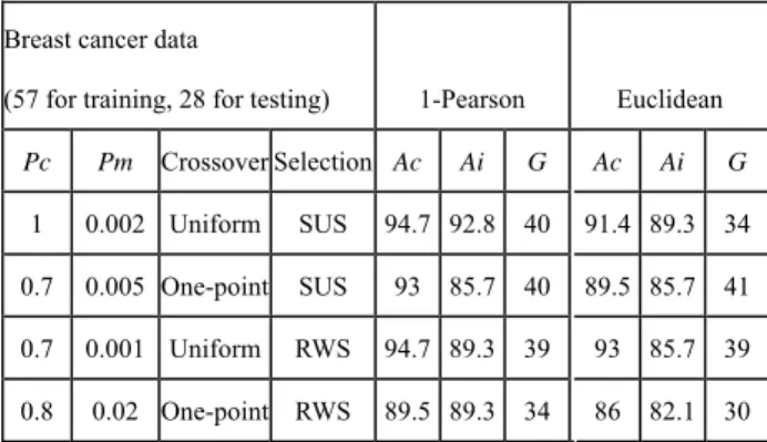
In Table 2, we have tried many groups of GA parameters for possible prediction performances. The best prediction accuracy was achieved using the Uniform crossover and SUS selection strategy of GA. The best predictor set

obtained from our method exhibits LOOCV accuracy (Ac)

of 94.7% in comparison with the cross validation success rate of 89% by the BSS/WSS/SVM [14]. Even in diagnosing blind test samples our method needed only 40

predictive genes to produce independent test accuracy (Ai)

of 92.8%, whereas BSS/WSS/SVM only performed cross

validation tests and needed hundreds of predictive genes. Table 2： Accuracy measured in percentage

Breast cancer data

(57 for training, 28 for testing) 1-Pearson Euclidean

Pc Pm Crossover Selection Ac Ai G Ac Ai G 1 0.002 Uniform SUS 94.7 92.8 40 91.4 89.3 34 0.7 0.005 One-point SUS 93 85.7 40 89.5 85.7 41 0.7 0.001 Uniform RWS 94.7 89.3 39 93 85.7 39 0.8 0.02 One-point RWS 89.5 89.3 34 86 82.1 30 3.2、Classification confidence

The silhouette statistics can be used to assess the quality of clustering by measuring how well an object is assigned to its corresponding cluster. According to the 40 predictor genes obtained above, Figure 2 shows the prediction confidence of each sample classified.

0 5 10 15 20 25 30 35 40 45 50 55 60 -0.4 -0.3 -0.2 -0.1 0 0.1 0.2 0.3 0.4 Training Samples S ilh o u e tte V a lu e basal-like ERBB2+ normal basal-like luminal A luminal B luminal C (A) 0 4 8 12 16 20 24 28 -0.4 -0.3 -0.2 -0.1 0 0.1 0.2 0.3 0.4 Testing Samples Si lhouet te V a lu e basal-like ERBB2+ normal basal-like luminal A luminal B luminal C (B)

Figure 2 ： The silhouette value for (A) training samples and (B) testing samples.

3.3、Meaningful genes for breast cancer data

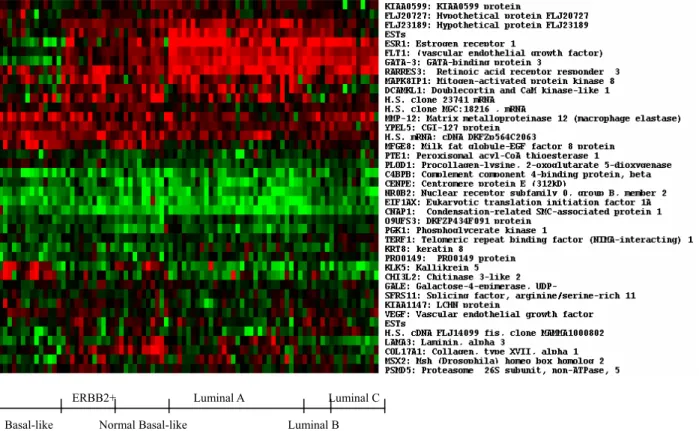
From the best result through our method, the heatmap of Figure 3 identifies the filtered 40 genes to reveal potential tumor subclasses and their associated biomarkers. Despite the lack of a broader investigation of these genes, below we list some informative genes and describe their relationships with breast cancers.

(1). ESR1 is a valuable predictive factor to help individualize therapy of breast cancer since its gene amplification is frequent in breast tumor cells. (2). FLT1 and VEGF express more abundant in cancer

cases with metastases than in cases without metastases.

(3). RARRES3 gene overexpression inhibits the growth of many cell lines, and it may function as an antiproliferative and antitumor agent.

(4). MMP12 is a proteolytic enzyme. It can be evaluated the association of breast cancer risk and survival with two common polymorphisms in the MMP12 gene: A-82G in the promoter region and A1082G in exon.

(5). GATA-3 is a significant predictor of overall survival.

(6). TERF1 encodes a telomere specific protein which functions as an inhibitor of telomerase to maintain

chromosomal stability.

(7). KRT8 expresses in the breast epithelium, but at

higher levels in the luminal than in the basal

component.

(8). Kallikrein 5 is a potential novel serum biomarker for breast and ovary cancers.

(9). PGK1 is a prognostic biomarker that differentially expresses in ERBB2+ breast tumors.

Figure 3：Expression profiles of predictor genes (40 genes) from experimental dataset. The x-axis denotes the tumor types. The name and brief descriptions of the predictor genes are shown along the y-axis. The intensity of red colored small squares represents the degree of up-regulated gene expression and the intensity of green color represents down-regulated gene expression as well as the black color represents unchanged expression levels.

4、Conclusions

In this paper, we propose a genetic algorithm adopting silhouette statistics with correlation metrics for gene selection and pattern classification. Experimental results prove the effectiveness and superiority of our method to improve the prediction accuracy and to reduce the number of predictive genes. Furthermore, we not only identify many predictors that are already known to be important for breast cancers, but also find many potential

targets for further biomarker researches. Finally, we hope that the proposed method would be a helpful tool that can be applied to analysis of mircroarray data for cancer diagnosis in clinical practice.

References

[1] A.A. Alizadeh, M.B. Eisen, R.E. Davis, C. Ma, I.S. Lossos, A. Rosenwald, J.C. Boldrick, H. Sabet, T. Tran, X. Yu et al., “Distinct types of diffuse large

ERBB2+ Luminal A Luminal C Basal-like Normal Basal-like Luminal B

B-cell lymphoma identified by gene expression profiling”, Nature, Vol. 403, pp. 503–511, 2000. [2] A. Ben-Dor, N. Friedman, and Z. Yakhini, “Scoring

genes for relevance”, Technical Report AGL-2000-13 Agilent Laboratories, 2000.

[3] J.M. Deutsch, “Evolution algorithms for finding optimal gene sets in microarray prediction”, Bioinformatics, Vol. 19, pp. 45–52, 2003.

[4] P. Fortina, S. Surrey, and L.J. Krica, “Molecular diagnosis: hurdles for clinical implementation”, Trends Mol. Med., Vol. 8, pp. 264–266, 2002. [5] T. Furey, N. Cristianini, N. Duffy, D. Bednarski, M.

Schummer, and D. Haussler, “Support vector machine classification and validation of cancer tissue samples using microarray expression data”, Bioinformatics, Vol. 16, pp. 906–914, 2000.

[6] T.R. Golub, D.K. Slonim, P. Tamayo, C. Huard, M. Gaasenbeek, J.P. Mesirov, H. Coller, M.L. Loh, J. Downing, M.A. Caligiuri, C.D. Bloomfield, and E.S. Lander, “Molecular classification of cancer: class discovery and class prediction by gene expression monitoring”, Science, Vol. 286, pp. 531–537, 1999. [7] L. Kaufman, and P.J. Rousseeuw, “Finding Groups

in Data: An Introduction to Cluster Analysis”, Wiley, New York, 1990.

[8] J.J. Liu, G. Cutler, W. Li, Z. Pan, S. Peng, T. Hoey, L. Chen, and X.B. Ling, “Multiclass cancer classification and biomarker discovery using GA-based algorithms”, Bioinformatics, Vol. 21, pp. 2691–2697, 2005.

[9] L. Li, C.R. Weinberg, T.A. Darden, and L.G. Pedersen, “Gene selection for sample classification based on gene expression data: study of sensitivity to choice of parameters of the GA/KNN method”, Bioinformatics, Vol. 17, pp. 1131–1142, 2001. [10] T. Li, C. Zhang, and M. Ogihara, “A comparative

study of feature selection and multiclass classification methods for tissue classification based on gene expression”, Bioinformatics, Vol. 20, pp. 2429–2437, 2004.

[11] E.E. Ntzani, and J.P. Ioannidis, “Predictive ability of DNA microarray for cancer outcomes and correlates: and empirical assessment”, Lancet, Vol. 362, pp. 1439–1444, 2003.

[12] C.H. Ooi, and P. Tan, “Genetic algorithms applied to multi-class prediction for the analysis of gene expression data”, Bioinformatics, Vol. 19, pp. 37–44, 2003.

[13] D.K. Slonim, P. Tamayo, J.P. Mesirov, T. Golub, and E. Lander, “Class prediction and discovery using gene expression data”, Proceedings of The Fourth Annual International Conference on Computational Molecular Biology, Universal Academy Press, Japan, 2002, pp. 263–272.

[14] G.S. Shieh, C.H. Bai and C. Lee, “Identify Breast Cancer Subtypes by Gene Expression Profiles”, Journal of Data Science, Vol. 2, pp. 165-175, 2004. [15] T. Speed, “Statistical Analysis of Gene Expression

Microarray data”, Chapman & Hall/CRC, New York, 2003.

[16] T. Sorlie, C.M. Perou, and R. Tibshiranie, et. al, “Gene expression patterns of breast carcinomas distinguish tumor subclasses with clinical implications”, PNAS, Vol. 98, pp. 10869-10874, 2001.