一個在無線區域網路上增進VoIP傳輸效能的適應性輪詢機制

國立交通大學

資訊科學與工程研究所

碩士論文

一個在無線區域網路上增進 VoIP 傳輸效能的適

應性輪詢機制

An Adaptive Polling Scheme for Improving VoIP

Transmission Performance over Wireless LANs

研 究 生 : 艾許拉夫

指導教授 : 陳耀宗 教授

一個在無線區域網路上增進 VoIP 傳輸效能的適應

性輪詢機制

An Adaptive Polling Scheme for Improving VoIP

Transmission Performance over Wireless LANs

研 究 生 : 艾許拉夫

Student : Ashraf Milhim

指導教授 : 陳耀宗

Advisor : Yaw-Chung Chen

國 立 交 通 大 學

資訊科學與工程研究所

碩 士 論 文

A Thesis

Submitted to Department of Computer Science College of Computer Science

National Chiao Tung University in partial Fulfillment of the Requirements

for the Degree of Master

in

Computer Science August 2006

Hsinchu, Taiwan, Republic of China

Table of Contents

List of Figures... ii

List of Tables ... iii

中文摘要... iv

Abstract... v

Acknowledgement ... vi

Chapter 1 Introduction... 1

Chapter 2 Background and Related Work... 6

2.1 Review of IEEE 802.11 MAC... 6

2.1.1 Distributed Coordination Function... 6

2.1.1 Point Coordination Function ... 9

2.2 Introduction to IEEE 802.11e ... 11

2.2.1 Enhanced Distributed Channel Access (EDCA) ... 12

2.2.2 HCF Controlled Channel Access (HCCA) ... 15

2.3 Comparison between WLAN MACs ... 18

2.4 Voice Transmission Requirements over WLANs ... 19

2.5 Related Works... 21

Chapter 3 Problem Definition... 22

3.1 Introduction... 22

3.2 Fairness polling ... 23

3.3 Polling overhead... 24

3.4 Delay... 24

Chapter 4 Proposed Adaptive Polling Scheme... 27

4.2 Scheme Architecture... 27

4.3 The motivation of using two lists ... 29

4.3.1 The talking list structure ... 29

4.3.2 The silence list structure... 30

4.4 Updating polling lists ... 30

4.4.1 Silence detection ... 31

4.4.2 Reordering the lists ... 34

4.5 TXOP Calculation... 36

4.6 Polling the talking and silence lists... 37

4.6.1 Polling the talking list ... 37

4.6.2 Polling silence list ... 38

Chapter 5 Simulations and results ... 39

5.1 Simulation environment ... 39

5.2 Simulation results... 39

5.2.1 Throughput... 40

5.2.2 Delay... 41

5.2.3 Packet loss ratio... 42

5.2.4 Polling Overhead analysis ... 43

Chapter 6 Conclusion and Future Work ... 45

List of Figures

Figure 2.1: Backoff mechanism of BEB………...7

Figure 2.2: Interframe Spacing Relationship...8

Figure 2.3: DCF timing chart...8

Figure 2.4: The CFP and CP timeline...10

Figure 2.5: An example of PCF operation...11

Figure 2.6: IEEE 802.11 Protocol layer...12

Figure 2.7: IEEE 802.11eEDCA mechanism parameters...13

Figure 2.8: IEEE 802.11 EDCA channel access procedure...14

Figure 2.9: The mechanism of EDCA...14

Figure 2.10: Example of HCCA frame exchange sequence...16

Figure 2.11: HCCA mechanism...17

Figure 2.12: Sample schedule with the reference scheduler...18

Figure 3.1: A two-state Markov chain voice activity model ………...23

Figure 3.2: Delay average against network size for RR using HCF...25

Figure 3.3: Packet loss ratio against network size using HCF...26

Figure 4.1: Architecture of the proposed scheme...28

Figure 4.2: Talking polling list...30

Figure 4.3: Silence polling list...30

Figure 4.4: A flow chart of initial silence detection...32

Figure 4.5 a: Talking list management...33

Figure 4.5 b: Silence list management...34

Figure 5.1: Total throughput against network size for Reference, APS, and RR schedulers...40

Figure 5.2: Average delay against network size for Reference, APS, and RR schedulers...41

Figure 5.3: Packet loss ratio against network size for Reference, APS, and RR schedulers...42

List of Tables

Table 1.1: The IEEE 802.11 family...2

Table 2.1: UP to AC mapping...12

Table 2.2: QoS frames. ...16

Table 2.3: Speech Coding Standards...20

Table 4.1: TSPEC direction field is a two bits field to specify the direction of traffic………...31

Table 4.2: Priorities of stations in polling lists...35

Table 5.1: MAC and physical parameters...39

一個在無線區域網路上增進

VoIP 傳輸效能的適應性輪詢機制

學生 : 艾許拉夫 指導教授 : 陳耀宗 教授

國立交通大學資訊工程學系﹙研究所﹚碩士班

中文摘要

隨著網路電話，以及無線網路系統的逐漸普及，將兩者結合為無線

網路電話也將是未來的必然新趨勢。隨著這個趨勢的發展，無線網路

標準

IEEE 802.11e 便孕育而生了，它保證了在無線網路上的服務傳輸

品質，這對於語言的傳遞這種敏感度較高的應用尤其重要。它提供了

一種新的介面傳輸方式命名為

HCF，它用來解決 IEEE 802.11 中舊有的

DCF 以及 PCF。為了要減少傳輸時間的延遲以及在各無線裝置間的輪

巡的時間，我們提出了一個新的輪巡方式，它是在

HC 端以 HCCA 的

模式下運行，其中，HC 中會將所有與之相連的無線設備分為兩類並將

之分別記錄起來，其中一類為運作中的設備，另一類為非運作中的設

備，這兩筆記錄除了會隨著目前的狀況做動態的更新，還會依據

HC 和

各無線裝置的傳輸方向和等候列中的情況，去做最正確的記錄和排

列。我們提出了一個簡單的方式去判定無線裝置是否是在運作的狀

態，這種方法我們稱為

VBR 和 CBR。運作中設備的 TXOP 是和非運作

中設備是分開做排程的。而後，HC 會在這兩大類設備的記錄中去做輪

巡。從模擬的結果可以清楚的看到，輪巡所花費的時間，已經減少很

多了，因此我們可以得到多放傳統方式的資料傳輸量，以及少的傳輸

延遲時間。

An Adaptive Polling Scheme for Improving VoIP

Transmission Performance over Wireless LANs

Student: Ashraf Milhim Advisor: Yaw-Chung Chen

Department of Computer Science

National Chiao Tung University

Abstract

Motivated by the promising voice over IP technology, and the wide service availability of WLANs, the application of VOWLAN is expected to experience dramatic growth in the near future. IEEE 802.11e standard was established to guarantee a high level of QoS especially for the time sensitive applications, such as voice services. It introduced a new medium access mechanism HCF in order to solve the QoS provisioning problem in the legacy IEEE 802.11 and its two medium access mechanisms of DCF and PCF. In order to reduce access delays and polling overhead, as well as to enhance the throughput of the channel, we propose an adaptive polling scheme, which works on the HC side in HCCA mode, in which, HC maintains two dynamic polling lists, one contains talking stations and the other contains silence stations, those lists are updated dynamically in order to classify stations into several levels of priority, they are reordered and sorted according to the traffic direction and the queue occupancy on the HC and the station. Stations are classified to be talking or silent according to a simple silence detection mechanism. VBR and CBR codecs are taken into consideration in our silence detection mechanism. TXOPs for stations in the talking list are calculated separately from the TXOPs for stations in silence list. HC then polls stations in both lists in a Round-Robin manner starting from the top of polling list and ending with the tail of silence list. Simulation results show that the polling overhead is reduced significantly, in addition to a high throughout and low access delays comparing to the classical Round-Robin polling scheme and the reference scheme in the standard.

Acknowledgement

First of all, I would like to express my sincerity to Prof. Yaw-Chung Chen, who supported me with all of his rich experience, precious time and for his enthusiastic guidance to complete this thesis. Also I would like to thank my family who put all of their trust in me and supported me all the time. I deeply thank all of my lab mates who encouraged me to keep going and complete my work, especially Bashar and Chun-Yung Lin. Finally I would like to thank my fiancée, who kept pushing and encouraging me all the time.

Chapter 1 Introduction

Deployments of wireless networks (WLANs) have grown rapidly in the last few years, it can prove to be very useful in public places – libraries, guest houses, hotels, cafeterias, airports, and schools are all places where one might find wireless access to the Internet. Nowadays most of handheld devices such as notebooks, tablet PCs, and PDAs are provided by one or more built-in wireless interfaces, users can access internet without the need to install any wires.

IEEE 802.11 is the most popular protocol amongst other wireless protocols such as Bluetooth, WiMAX, and UWB. The 802.11 working group was established in 1990 by the IEEE Executive Committee. Their goal was to create a wireless local area network (WLAN) standard. The standard specified an operating frequency in the 2.4GHz ISM (Industrial, Scientific, and Medical) band. Seven years later (1997), the group approved IEEE 802.11 as the world's first WLAN standard with data rates of 1 and 2 Mbps. In 1999 the working group approved two extensions to 802.11, the first one is 802.11a operates on U-NII band (Unlicensed National Information Infrastructure) 5GHz, and with a maximum bandwidth of 54 Mbps (due to higher frequency), it only allow access to clients within 40 – 50 feet due to power limits enforced by the FCC, while the second extension is 802.11b which operates on 2.4GHz ISM band, with a maximum bandwidth of 11 Mbps, it allows client access up to well over 1000 feet. The whole Family of IEEE 802.11 is shown in Table 1.1.

Ad Hoc mode and Infrastructure mode are most common wireless configurations found today. Ad Hoc mode (which also referred to as “Independent Basic Service Set” (IBSS)) provides peer-to-peer communication links between two or more wireless devices without the use of an AP, while Infrastructure mode (which is also known as “Basic Service Set” (BSS)) requires an Access Point and at least one wireless client.

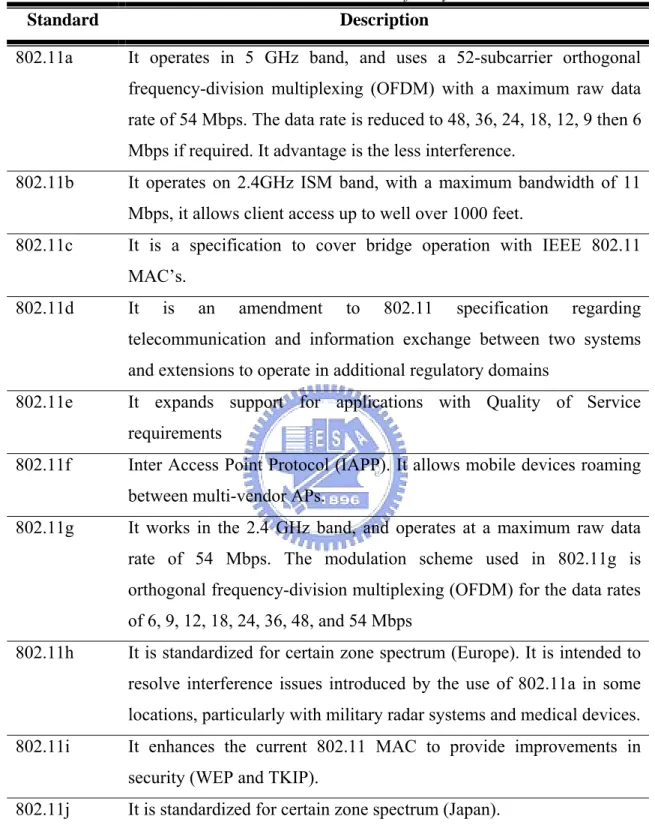
Table 1.1: The IEEE 802.11 family.

Standard Description

802.11a It operates in 5 GHz band, and uses a 52-subcarrier orthogonal frequency-division multiplexing (OFDM) with a maximum raw data rate of 54 Mbps. The data rate is reduced to 48, 36, 24, 18, 12, 9 then 6 Mbps if required. It advantage is the less interference.

802.11b It operates on 2.4GHz ISM band, with a maximum bandwidth of 11 Mbps, it allows client access up to well over 1000 feet.

802.11c It is a specification to cover bridge operation with IEEE 802.11 MAC’s.

802.11d It is an amendment to 802.11 specification regarding telecommunication and information exchange between two systems and extensions to operate in additional regulatory domains

802.11e It expands support for applications with Quality of Service requirements

802.11f Inter Access Point Protocol (IAPP). It allows mobile devices roaming between multi-vendor APs.

802.11g It works in the 2.4 GHz band, and operates at a maximum raw data rate of 54 Mbps. The modulation scheme used in 802.11g is orthogonal frequency-division multiplexing (OFDM) for the data rates of 6, 9, 12, 18, 24, 36, 48, and 54 Mbps

802.11h It is standardized for certain zone spectrum (Europe). It is intended to resolve interference issues introduced by the use of 802.11a in some locations, particularly with military radar systems and medical devices. 802.11i It enhances the current 802.11 MAC to provide improvements in

security (WEP and TKIP).

802.11j It is standardized for certain zone spectrum (Japan).

Recently, Voice over Internet Protocol (VoIP) became one of the most popular Internet applications. Some products of VoIP like Skype and MSN are able to guarantee a high level of voice quality over wired networks. The popularity of VoIP comes from its

low cost and good quality, thus, people can use their PCs to make calls instead of the expensive cell phone calls, statistics says that the number of residential VoIP users will rise from three million at 2005 to 27 million by the end of 2009[17].

To provide person-to-person (instead of place-to-place) connections anywhere and anytime, the Internet is expected to penetrate the wireless domain. One very promising wireless network is the wireless local area network (WLAN), which has shown the potential to provide high-rate data services at low cost over local area coverage. However, Voice over 802.11 (VO802.11) faces a lot of challenges to guarantee a high level of quality, such as low bandwidth, large interference, long latency, high loss rates, and jitter, so we need to enhance the 802.11 standard to be able to support VoIP with a high level of voice quality. Furthermore, the distributed coordination function (DCF) and the point coordination function defined in basic IEEE 802.11 are unsuitable to guarantee QoS effectively.

As a solution of the Quality of Service problem facing the VO802.11, the IEEE 802.11 group chartered the 802.11e task group with the responsibility of enhancing the 802.11 Medium Access Control (MAC) to include bidirectional QoS to support latency-sensitive applications such as voice and video. The new standard of IEEE 802.11e [1] is expected to solve the QoS problem of real-time applications over wireless local area networks.

IEEE 802.11e has brought many enhancements, some are general and some are specific. The first general enhancement is the option to allow stations to talk directly to other stations, bypassing the AP, even when there is one. The second general enhancement is the introduction of negotiable acknowledgements, IEEE 802.11e introduces the notion of negotiable acknowledgements whereby a packet in a stream need not to be acknowledged, or such acknowledgements can be aggregated depending on the parameterization of a stream, such negotiable acknowledgements lead to a more efficient utilization for the available channel and enable applications such as a reliable multicast. And the third general enhancement is the introduction of traffic parameterization and traffic prioritization. These are central to any QoS mechanism. The major novelty developed by IEEE 802.11e is the new coordination function called Hybrid-Coordination Function (HCF). It is a coordination function that combines aspects of the distributed

coordination function and the point coordination function. HCF uses a contention-based channel access method, called the Enhanced Distributed Channel Access (EDCA). Because it operates in the contention period, EDCF is similar to DCF. QoS support is realized with the introduction of the Traffic Categories (TCs). However, EDCA doesn’t guarantee QoS of time sensitive applications. The second mechanism for access to the wireless medium, which is part of the HCF, is called HCF-Controlled Channel Access (HCCA). It provides the capability for reservation of transmission opportunities (TXOPs) with the HC. This mechanism is expected to be used for the transfer of periodic traffic such as voice and video. HCCA operates on Contention Free Periods (CFPs) or it can be invoked during Contention Periods (CPs). HCF is based on polling, so it is a modified version of PCF, it is promising to guarantee QoS of real-time applications. HCCF is a little complex to be implemented and many researches are still in progress.

HCCA polling mechanism is still unspecified in the standard, polling scheduling in HCCA is left to designers till now. The study in [2] shows the polling overhead problem and its negative effect on the QoS of voice streams in WLANs. An effective polling scheduler will extremely enhance the performance, and assure a high level of QoS for the time sensitive applications. The most popular polling mechanism mentioned in [6] is the round robin mechanism, it is popular due to the simplicity if its implementation. Many other polling schemes have been proposed such as [4], [5], and [7].

In our study we focus on HCCA, on its polling scheduler in particular. We proposed a new scheduler called Adaptive Polling Scheme (APS), the proposed scheduler showed a high performance against the other schedulers. APS depends on prioritizing voice stations according to their state using a simple mechanism of silence detection, and on the queue occupancy at both the AP side and the station side. In addition to its role in scheduling the order of stations and calculating TXOPs, it works as a queue management scheme to prevent full queues on the AP and to prevent stations from dropping packets of their voice traffic category. In APS we maximized the usage of piggybacking feature of IEEE 802.11e, to increase the total throughput of the wireless channel. Here we proposed two dynamic polling lists, one contains the information of the stations in talking state while the other contains the information of the stations in the silent state, each station has its own order in the polling lists, since each one of the two polling list is sorted according

to different criteria, the talking list is sorted according to the occupancy percentage at the AP transmission queues and at the station traffic categories calculated by giving those occupancies different weights, while silence list is sorted according to the occupancy percentage of the transmission queues at the AP only.

The rest of this thesis is organized as follows. Chapter 2 introduces the background of IEEE 802.11 and IEEE 802.11e, voice transmission requirements on WLANs, and a brief survey of current polling mechanisms. Chapter 3 points to the problem definition that motivated us to do this work. In chapter 4, we discuss the proposed adaptive polling scheme. We demonstrate our simulation and analytical results in chapter 5. Finally the conclusion and future works are presented in chapter 6.

Chapter 2 Background and Related Work

In this chapter we will review IEEE 802.11 and IEEE 802.11e, including their medium access mechanisms. Then we will go through the advantages and disadvantages of WLANs MACs. We will also give a brief background about voice transmission requirements, including a review of voice codecs and how do they work, furthermore. Finally, we will list some related works that have been proposed.

2.1 Review of IEEE 802.11 MAC

Access to the wireless medium is controlled by coordination functions. Ethernet-like CSMA/CA access is provided by the distributed coordination function (DCF). If contention-free service is required, it can be provided by the point coordination function (PCF), which is built on top of the DCF. Contention-free services are provided only in infrastructure networks. The coordination functions are described in the following list.

2.1.1 Distributed Coordination Function

Distributed Coordination Function (DCF) is the fundamental access mechanism in the IEEE 802.11 MAC. In this section we will briefly describe the basic access mechanism of DCF. When a node (station) has a packet to transmit, it senses whether the medium has been idle for a period of time no shorter than the Distributed InterFrame Space (DIFS), the packet transmission may begin immediately at the beginning of the following slot. Otherwise, the node should defer the packet transmission as follows, The node waits until the medium is idle for a DIFS and then sets its backoff timer. The backoff timer is set to a value which is randomly selected from 0, 1, …, CW-1 with equal probability, where CW represents contention window size. Initially, contention window size is set to its minimum CWmin for the first transmission attempt of a packet. Every time

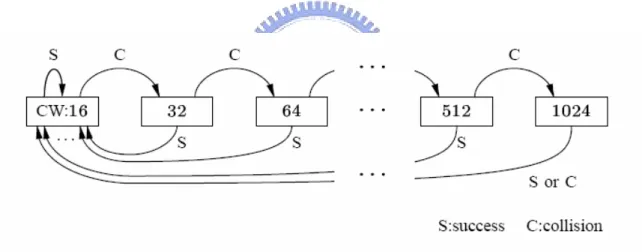
the packet is involved in a collision, contention window size is doubled for the next transmission attempt. However, the contention window size cannot exceed its maximum CWmax. The backoff timer is decreased by 1 every slot time (50 µsec for FHSS PHY) after the medium has been idle for a DIFS, but is frozen when the medium becomes busy. When the backoff timer becomes zero, the station transmits the packet. If the destination node receives the packet correctly, it sends a positive acknowledgment (ACK) packet after a Short InterFrame Space (SIFS). When the source node does not receive an ACK, it assumes that the packet has experienced a collision and updates the contention window size CW according to Binary Exponential Backoff (BEB) algorithm as illustrated in Figure 2.1, then sets its backoff timer to a newly selected backoff values after an Extended InterFrame Space (EIFS). Since the number of transmission retries is bounded by threshold m, a packet must be dropped after m transmission retries, that is, after experiencing m times of packet collision.

Figure 2.1: Backoff mechanism of BEB: CWmin = 16, CWmax = 1024, m = 7. As with traditional Ethernet, the interframe spacing plays an important role in coordinating access to the transmission medium. 802.11 uses four different interframe spaces. Three are used to determine medium access; the relationship between them is shown in Figure 2.2.

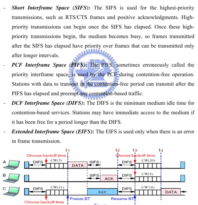
Figure 2.2: Interframe Spacing Relationship. The interframe space times in IEEE 802.11 are:

- Short Interframe Space (SIFS): The SIFS is used for the highest-priority transmissions, such as RTS/CTS frames and positive acknowledgments. High-priority transmissions can begin once the SIFS has elapsed. Once these high-priority transmissions begin, the medium becomes busy, so frames transmitted after the SIFS has elapsed have priority over frames that can be transmitted only after longer intervals.

- PCF Interframe Space (PIFS): The PIFS, sometimes erroneously called the priority interframe space, is used by the PCF during contention-free operation. Stations with data to transmit in the contention-free period can transmit after the PIFS has elapsed and preempt any contention-based traffic.

- DCF Interframe Space (DIFS): The DIFS is the minimum medium idle time for contention-based services. Stations may have immediate access to the medium if it has been free for a period longer than the DIFS.

- Extended Interframe Space (EIFS): The EIFS is used only when there is an error in frame transmission.

2.1.1 Point Coordination Function

As an optional access method, the 802.11 standard defines the PCF, which enables the transmission of time-sensitive information. With PCF, a point coordinator within the access point controls which stations can transmit during any given period of time. Within a time period called the contention free period, the point coordinator will step through all stations operating in PCF mode and poll them one at a time. For example, the point coordinator may first poll station A, and during a specific period of time station A can transmit data frames (and no other station can send anything). The point coordinator (PC) will then poll the next station and continue down the polling list, while letting each station to have a chance to send data. Thus, PCF is a contention-free protocol and enables stations to transmit data frames synchronously, with regular time delays between data frame transmissions. This makes it possible to more effectively support information flows, such as video and control mechanisms, having strict synchronization requirements.

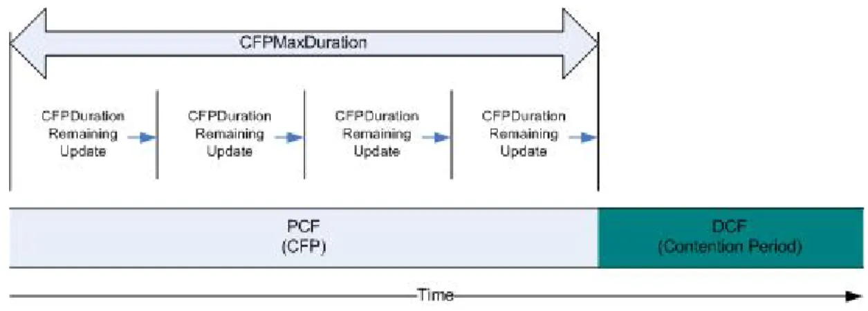
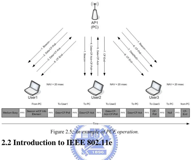
The contention Free Period (CFP) is the window of time for PCF operation. The CFP begins at setting intervals following a beacon frame which contains a delivery traffic indication map (DTIM) information element. The frequency of CFPs is determined by the network administrator. Once the CFP begins, the AP assumes the role of PC (and as such, PCF operation is only supported in infrastructure BSSs). Each 802.11 client sets its NAV to the CFPMacDuration value. This value is included in the CF parameter set information element. The CFPMaxDuration defines the time value that is the maximum duration for the CFP. The PC can end the CFP before the CFPMaxDuration time elapsed. The AP transmits beacon frames at regular intervals, and beacon frames sent during the CFPDurationRemaining field to update station NAVs of the remaining duration of the CFP. Figure 2.4 depicts the CFP and contention period as a function of time. Unlike DCF operation, DCF doesn’t allow station to freely access the medium and transmit data. Stations can only send data (one frame at a time) when the PC polls them. The PC can send frames to stations, poll stations for frame transmission, acknowledge frames requiring MAC-level Acknowledgements, or end the CFP.

Figure 2.4: The CFP and CP timeline.

When the CFP begins, the PC must access the medium in the same manner as a DCF station. Unlike DCF stations, the PC attempts to access the medium after waiting an interval of PIFS. The PIFS interval is one slot time longer than SIFS interval and one slot time shorter than the DIFS interval, allowing PCF stations to access the medium before DCF stations yet still allowing control frames, such as acknowledgement frames, to have the highest probability of gaining access to the medium. After waiting a PIFS interval, the PC sends the initial beacon containing the CF parameter information element. The PC waits for one SIFS interval subsequent to the beacon frame transmission and then sends one of the following to a CF-Pollable station:

• A data frame

• A Poll frame (CF-Poll)

• A combination data and poll frame (Data+CF-Poll) • A CFP end frame (CF-End)

If the PC has no frames to send and no CF-Pollable stations to poll, the CFP is considered null, and immediately following the beacon frame, the PC sends a CF-End frame for terminating the CFP. An example of PCF is shown in Figure 2.5.

The time period for a PC to generate beacon frames is called target beacon transmission time (TBTT). Usually, PCF uses a round-robin scheduler to poll each station sequentially in the order of the polling list, but priority-based polling mechanisms can also be used if different QoS levels are requested by different stations.

Figure 2.5: An example of PCF operation.

2.2 Introduction to IEEE 802.11e

IEEE 802.11 MAC can’t guarantee the Quality of Service (QoS) for time sensitive applications such as audio and video applications, and it faces the problems of high level of quality, such as low bandwidth, large interference, long latency, high loss rates [18], and jitter. To solve the problems of QoS , the IEEE 802.11 group chartered the 802.11e task group with the responsibility of enhancing the 802.11 Medium Access Control (MAC) to include bidirectional QoS to support latency-sensitive applications such as voice and video. The new standard of IEEE 802.11e [1] is expected to solve the QoS problem of real-time applications over wireless local area networks. IEEE 802.11e has brought many enhancements, some are general and some are specific. The first general enhancement is the option to allow stations to talk directly to other stations, bypassing the AP, even when there is one, which is called the Direct Link Protocol (DLP). The second general enhancement is the introduction of negotiable acknowledgements. And the third general enhancement is the introduction of traffic parameterization and traffic

function called Hybrid-Coordination Function (HCF). It is a coordination function that combines aspects of the distributed coordination function and the point coordination function. HCF uses a contention-based channel access method, called the Enhanced Distributed Channel Access (EDCA), and a contention-free-based mechanism for access to the wireless medium is called HCF-Controlled Channel Access (HCCA). The relationship between IEEE 802.11 and IEEE 802.11e is shown in Figure 2.6.

Figure 2.6: IEEE 802.11 Protocol layer.

2.2.1 Enhanced Distributed Channel Access (EDCA)

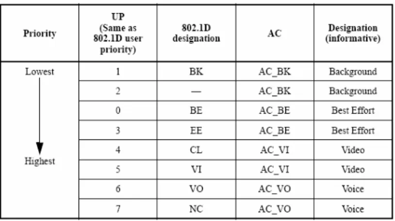
EDCA is designed to enhance the DCF mechanism and to provide a distributed access method that can support service differentiation among classes of traffic. The EDCA mechanism provides differentiated, distributed access to the WM for QSTAs using eight different User Priorities (UPs). The EDCA mechanism defines four access categories (ACs) that provide support for the delivery of traffic with UPs at the QSTAs. The AC is derived from the UPs as shown in Table 2.1.

EDCA assigns smaller CWs to ACs with higher priorities to bias the successful transmission probability in favor of high-priority ACs in a statistical sense. Indeed, the initial CW size can be set differently for different priority ACs, yielding higher priority ACs with smaller CW. To achieve differentiation, instead of using fixed DIFS as in the DCF, an AIFS is applied, where the AIFS for a given AC is determined by the following equation:

AIFS = SIFS + AIFSN x aSlotTime (2.1)

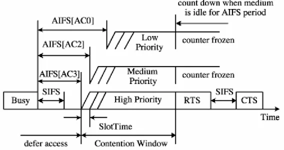
Where AIFSN is AIFS Number and determined by the AC and physical settings, and aSlotTime is the duration of a time slot. The AC with the smallest AIFS has the highest priority. Figures 2.7 and 2.8 illustrate these EDCA parameters and the access procedure, respectively.

Figure 2.7: IEEE 802.11eEDCA mechanism parameters.

In the EDCA, both the physical carrier sensing and the virtual sensing methods are similar to those in the DCF. However, there is a major difference in the countdown procedure when the medium is determined to be idle. In the EDCA, after the AIFS period, the backoff counter decreases by one at the beginning of the last slot of the AIFS (shown as the crossed time slot in Figure 2), while in the DCF, this is done at the beginning of the first time slot interval following the DIFS period.

Figure 2.8: IEEE 802.11 EDCA channel access procedure.

For a given station, traffic of different ACs are buffered in different queues as shown in Figure 2.9. Each AC within a station behaves like a virtual station: it contends for access to the medium and independently starts its backoff after sensing the medium idle for at least AIFS period. When a collision occurs among different ACs within the same station, the higher priority AC is granted the opportunity for physical transmission, while the lower priority AC suffers from a virtual collision, which is similar to a real collision outside the station.

IEEE 802.11e also defines a transmission opportunity (TXOP) limit as the interval of time during which a particular station has the right to initiate transmissions. During an EDCA TXOP, a station may be allowed to transmit multiple data frames from the same AC with a SIFS gap between an ACK and the subsequent data frame. This is also referred to as contention free burst (CFB).

Problem with EDCA

The throughput of each terminal can be calculated from the amount of sent/received frames per unit of time. Thus, if the numbers of terminals with high QoS priority increases, the frames transmission queue with a high AC value has a relatively longer waiting time for sending frames. Therefore, the allocated communication time of the wireless channel is not sufficient to guarantee the QoS communication for the requesting terminals. When the amount of sent/received frames per unit of time decreases, the throughput of each terminal decreases too. In public WLAN access environments, all users can use an unspecified number of APs to achieve the AP roaming, so the number of terminals accessing an AP varies over the time scale of hours to days. Therefore, we think that it is difficult for this method to guarantee QoS communication very well in public WLAN access environments [6].

2.2.2 HCF Controlled Channel Access (HCCA)

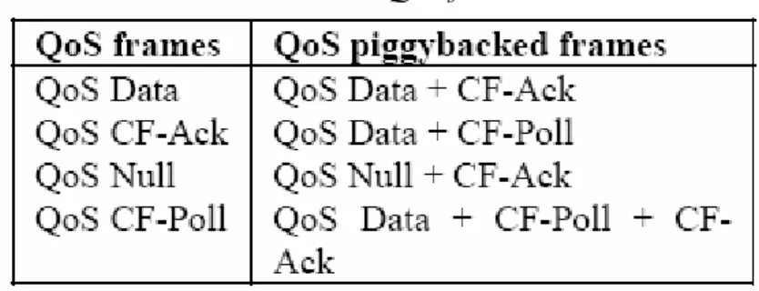
The HCCA is a centralized access mechanism controlled by the Hybrid Coordinator (HC), which resides in the QoS-enabled Access Point (QAP). Each QoS-enabled station (QSTA) may have up to eight established Traffic Streams (TS); a TS is characterized by a Traffic Specification (TSPEC) which is negotiated between the QSTA and the QAP. Mandatory fields of the TSPEC include: Mean Data Rate, Delay Bound, Maximum Service Interval, and Nominal SDU Size. For all established streams the QAP is required to provide a service that is compliant with the negotiated TSPEC under controlled operating conditions. 802.11e compliant stations must be able to process the additional frames reported in Table 2.2.

Table 2.2: QoS frames.

The QAP enforces the negotiated QoS guarantee by scheduling Controlled Access Phases (CAPs). A CAP is a time interval during which the QAP may either transmit MSDUs of established downlink TSs or poll one or more QSTAs by specifying the maximum duration of the transmission opportunity (TXOP): a QSTA is never allowed to exceed the TXOP limit imposed by the QAP, including interframe spaces and acknowledgments. If the traffic stream of a polled QSTA is not backlogged, then the QSTA responds with a Null frame. Figure 2.10 shows a sample CAP during which the QAP transmits two frames and polls the QSTA, which in turn transmits two frames. It is worth noting that the scheduling of CAPs, i.e. of HCCA traffic streams, also affects the overall capacity left to contention-based traffic, i.e. EDCA and DCF.

Figure 2.10: Example of HCCA frame exchange sequence.

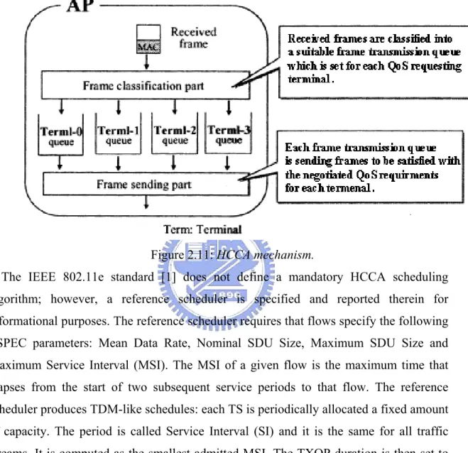
After the frame is received it is classified to be served by HCCA or EDCA, if it was classified to be served by HCCA then this frame must be enqueued into the appropriate transmission queue, since each Traffic Stream (TS) is assigned to a unique transmission

queue. Each one of those FIFO transmission queues contains packets to the station that initiated that TS. Figure 2.11 shows the HCCA mechanism.

Figure 2.11: HCCA mechanism.

The IEEE 802.11e standard [1] does not define a mandatory HCCA scheduling algorithm; however, a reference scheduler is specified and reported therein for informational purposes. The reference scheduler requires that flows specify the following TSPEC parameters: Mean Data Rate, Nominal SDU Size, Maximum SDU Size and Maximum Service Interval (MSI). The MSI of a given flow is the maximum time that elapses from the start of two subsequent service periods to that flow. The reference scheduler produces TDM-like schedules: each TS is periodically allocated a fixed amount of capacity. The period is called Service Interval (SI) and it is the same for all traffic streams. It is computed as the smallest admitted MSI. The TXOP duration is then set to the time required to transmit the packets of Nominal SDU Size that arrive at the negotiated Mean Data Rate during the SI; the TXOP is rounded up to contain an integer number of Nominal SDU Size. In order to avoid head of line blocking, the actual TXOP value is the maximum between the value obtained with the above procedure and the time to transmit a packet with Maximum SDU Size. A sample schedule showing three admitted flows (i, j and k) is demonstrated in Figure 2.12.

Figure 2.12: Sample scheduling with the reference scheduler.

2.3 Comparison between WLAN MACs

In this chapter we have reviewed two types of medium access mechanisms, the first type is a contention-based medium access mechanism, which includes the DCF and EDCA from the legacy IEEE 802.11 standard and the IEEE 802.11e standard respectively. The second type is contention-free-based or Polling-based medium access mechanism which includes PCF from legacy IEEE 802.11 and HCCA from IEEE 802.11e.

An advantage of Contention-based medium access mechanisms is that they are adaptive to the change in the network condition and are suitable for high load of traffic. Another advantage is the simplicity in implementation comparing with the polling-based medium access mechanism; this relative implementation simplicity comes as a result of the distributed access between the AP and the station. However, contention-based medium access mechanisms has some drawbacks, for example in EDCA case when the number of terminals of that are requesting QoS service increases, the other terminals should wait longer and longer, decreasing the sending/receiving rate for the lower priority transmission queues. Another drawback is that contention-based medium access mechanisms cannot guarantee QoS for time sensitive traffic, this comes from the randomness of selecting backoffs. Collision is another problem facing the contention-based medium access mechanisms, especially when using the same channel for transmitting or with the existence of hidden terminals.

Polling-based mechanisms have several advantages; one is eliminating the problem of hidden terminal. Another advantage is the guarantee of QoS for real-time traffic because of the centralized mechanism on the AP and the contention free transmission granted to stations by the AP. Channel utilization is much better because backoff overhead and collision problems are reduced. Nevertheless, the complexity of implementing polling-based mechanisms is much higher than implementing contention-based mechanisms. Finally, polling overhead is a drawback of polling-contention-based mechanisms especially if we compare the CF-Poll Packet transmission time with the voice transmission time.

2.4 Voice Transmission Requirements over WLANs

Voice application requirements are expressed in terms of QoS parameters with quantifiable values that can be determined from the application’s technical specification (i.e., Voice codec-ITU-T G.711) or from experimentation.

• Throughput: It is mostly expressed as the average data rate: o ITU-T G.711: 64 kbps

o ESTI GSM 6.10: 16 kbps o ITU-T G.727: Variable bit rate.

For applications that generate Variable Bit Rate (VBR) traffic, the average data rate doesn’t properly capture the traffic characteristics. Some voice codecs generates packets in VBR, which means that they generate voice packets while the station they work for is talking only. Constant Bit Rate codecs generate voice packets continuously every packetization interval, 5 ms, 10 ms, 20 ms, etc. VoIP requires relatively low bandwidth and the traffic pattern is relatively constant. Voice traffic is packetized in small packets of around 44 to 200 bytes resulting in short transmission times. Since voice conversations contain up to 60% silence [20], encoding algorithms yield lower bandwidth requirements with acceptable quality. Table 2.3 shows the speech coding standard. Mean Opinion Score (MOS) in Table 2.3 reflects the sound quality in quantitative way. MOS is an empirical

value determined by averaging the opinion score (i.e., the range from 1=worst to 5=best) of sample group of listeners who listen and evaluate the voice quality.

Table 2.3: Speech Coding Standards

Codec Bandwidth (kbps) Payload (bytes) Sound Quality (MOS) Packetization Interval (ms) ITU-T G.711 64 160 > 4 20 ITU-T G.722 48-64 - 3.8 - ITU-T G.723.1 6.4/5.3 20/24 3.9 30 ITU-T G.726 32 - 3.8 - ITU-T G.728 16 - 3.6 - ITU-T G.729 8 - 3.9 - GSM 06.10 13 33 3.5 50 GSM 06.20 5.6 - 3.5 - GSM 06.60 12.2 - > 4 - GSM 06.70 4.8 – 12.2 - > 4 -

• Delay and Delay jitter: The value is provided in a form of a bound (i.e., the delay should be less than a certain value). In delay intolerant applications, such as voice applications, the network has to follow the delay requirement strictly. However, in HCCA the station sends its delay bound value to the AP within a Traffic SPECefication (TSPEC) in order to inform it about the transmission requirements.

• Loss: it is mostly expressed as a statistical value (i.e., the percentage of loss packets should be less than a certain value).

2.5 Related Works

In our survey, we found that most of proposed polling mechanisms tried to find a mechanism in HCCA to avoid polling stations that have no packets to transmit in order to reduce the polling overhead and increase the channel efficiency [3], [4]. Another mechanisms proposed polling schemes with a silence detection mechanisms to avoid polling stations in silent state or delay them later after polling stations in talking state, for the VoIP traffic [2], [5]. Some other schemes proposed queue management mechanisms to reduce packet loss ratio on both station side and AP side like mechanism proposed in [11].

The survey in [7] reviews the most popular polling protocols and describes their advantages and drawbacks including polling list management mechanisms, determining the polling sequence, and minimizing polling overhead, then they propose a polling mechanism that aims to reduce packet loss ratio.

In [8] a full and comprehensive simulation is implemented for the reference scheduler proposed in the IEEE 802.11e standard [1].

In most of related works in our survey, researchers tried to avoid enforcing fairness in polling VoIP stations, and proposed schemes to differentiate between stations with download traffic (silence) and stations with upload traffic (talking) in order to reduce the polling overhead and delays, and improving the throughput of the transmission channel.

Chapter 3 Problem Definition

3.1 Introduction

The draft of IEEE 802.11e introduced a new medium access mechanism to guarantee a high level of QoS for the real time services, the working group E has proposed the Hybrid Coordination Function (HCF) as an enhancement to the legacy medium access functions: the Distributed Coordination Function (DCF) and the Point Coordination function. The DCF can’t guarantee QoS, while PCF can guarantee a low level of QoS but it still has some problems as described earlier in chapter 1. The HCF is a coordination function that combines aspects of the distributed coordination function and point coordination function, it consists of two medium access functions that work together: Enhanced Distributed Channel Access (EDCA) and HCF-Controlled Channel Access (HCCA). EDCA is an enhanced version of DCF, it is a contention based mechanism, while HCCA is an enhanced version of PCF that is contention free based and uses the polling mechanism to grant QoS stations the access to the medium for a limited amount of time calculated at the Hybrid Coordinator (HC), this time is called transmission opportunity (TXOP). IEEE 802.11e draft specifies neither a scheduling mechanism nor a polling mechanism for HCCA, and only an example that satisfies the minimum real time traffic requirements has been proposed, the scheduler has been left for designers. Although many scheduling mechanisms have been proposed, a lot of work still needs to be done to achieve an efficient scheduler.

In this chapter we will focus on some scheduling problems in general and on the Round-Robin (RR) polling mechanism in particular, we will discuss its weaknesses, and show its performance through simulations.

RR polling mechanism have some problems that we are going to discuss in this chapter, those problems are:

-

-

3.2 Fairness polling

In RR polling mechanism, HC polls stations sequentially in the order they are placed in the polling list. When the current polling round is over, the AP memorizes the place and starts polling it in the next round.

In a voice conversation users normally tend to stop their conversation, listen to their counter part and restart their conversation. The effect is known as the talkspurt-silence alternation, and the behavior is independent of the codec used and can be modeled by a two-state Markov chain as shown in Figure 3.1. The model is actually an ON/OFF stochastic process. The ON (talkspurt) and OFF (silence) periods are exponentially distributed with mean values 1/ α and 1/ β, respectively. During talk periods a voice flow is represented as an isochronous source with fixed inter-arrival time T that are determined by the audio codec. In other words, the packet generation rate λ is fixed. During silence period, nevertheless, no packets are generated.

Figure 3.1: A two-state Markov chain voice activity model.

The talkspurt-silence alternation characteristic of voice traffic makes RR polling mechanism not efficient at all. The reason is that the HC will neither add/delete station IDs in the polling list, nor change the sequence according to stations which are polled. As a result, although a certain voice source enters silence period, the still HC continues to poll it even the station responds NULL frame each time. This will cause wastage of

Talkspurt Silence

β α

valuable bandwidth wastage and incurs unnecessary delay to other stations in talkspurt state [17].

We see that when the HC enforces fair access to all stations regardless they were talking or silent, it wastes the resources that should be reserved for the talking stations with higher priority than the silent stations.

3.3 Polling overhead

In the IEEE 802.11e draft, overhead in HCF is due to frequent poll frames from the AP to mobile stations. The AP sends a QoS CF-Poll frame to each station (according to its polling list) one by one to grant the TXOP. However, this polling method is inefficient due to the large overhead. According to the IEEE 802.11 standard, the CF-Poll frame is required to be transmitted at the basic rate (2 Mb/s of IEEE 803.11b) regardless of the data rate. The size of CF-Poll frame is 36 bytes in the 802.11e draft, including 10 bytes for frame/sequence/QoS control and frame check sequence (FCS), 24 bytes for station ID, and 2 bytes for duration ID. Its transmission time at 2 Mb/s is 36 * 8/2 = 144 µs. Furthermore, considering the PHY overhead (192 µs), the total transmission time is 336 µs. The transmission time for a 196-byte voice packet (160-byte payload with a G711 codec and 36-byte MAC header) at 11 Mb/s data rate is 196*8/11 = 142.55 µs. Compared to the voice packet transmission time, the overhead contributed by the CF-Poll frame is relatively large. For a WLAN accommodating N voice users, the total overhead contributed by CF-Poll is 336 * N µs, which is significant [2]. Consider 40 voice users, half of them are talking and the other half are listening, to give any of them the permission to access the medium AP must send a QoS CF-Poll first, for the silent users who has no voice packets to send this poll is wasted and they are polled for nothing, and this poll is considered as overhead, 20*336 = 6720 µs. So we need a mechanism to avoid polling those stations with no buffered packets on their voice TC.

3.4 Delay

Polling silence stations wastes the time of receiving the null packet in addition to the time required to send the CF-Poll packet to the silent station, and by polling those silent stations frequently, longer and longer time is wasted, as a consequence of this

wasted time, talking stations will suffer long access delays, because they are enforced to wait until the HC poll all the stations before them in the polling list, which may be silent. Long delays may cause a high packet drop ratio on the station side. Talking station that is generating voice packets continuously may start dropping voice packets because of the long waiting time it may suffer.

Delay Average VS Network sieze

0 5 10 15 20 25 30 35 40 1 2 3 4 5 6 7 8 9 Number of stations D e la y A v er ag e ( m s) Round-robin

Figure 3.2: Delay average against network size for RR using HCF

We can notice in Figure 3.2, which we got from our simulation, the increasing delay due to the increase in the network size, which can be explained by the wasted polls to the silent stations and due to the high polling overhead. While Figure 3.3, which is a result of our simulation too, shows the packet loss ratio of RR for different network sizes, the increasing in packet loss ratio is noticeable; this increase is a result of the high access delays when the number of stations in the network is increased.

Packet Loss Ratio VS Network size 0 0.02 0.04 0.06 0.08 0.1 0.12 0.14 0.16 0.18 1 2 3 4 5 6 7 8 9 Number of stations P a cket L o s s R a ti o Round-robin

Figure 3.3: Packet loss ratio against network size using HCF

Chapter 4 Proposed Adaptive Polling Scheme

4.1 Overview

Based on the problems addressed in the previous chapter, in order to eliminate the problem of polling fairness and to minimize the packet loss ratio, polling overhead, and delay, we propose an Adaptive Polling Scheme (APS) to poll the VOIP stations on the HCCA mode efficiently. APS operates on the MAC sublayer of the HC. APS distinguishes between talking stations and silent stations and takes the transmission queues occupancy into consideration.

4.2 Scheme Architecture

The proposed APS maintains two polling lists, the first one is the talking polling list, it contains the Traffic Stream IDs (TSIDs) of the stations that are considered to be talking, while the second list is the silence polling list, which contains the TSIDs of the stations that are considered to be silent. APS consists of two modules, Silence Detector and List Manager (SDLM) module, and Polling Decision Maker (PDM) module.

Frames arriving at the HC’s MAC are classified first in order to be served by EDCA or HCCA, if a frame was classified to be served by HCCA, it should be enqueued into the appropriate transmission queue. Since each admitted stream is assigned to a transmission queue on the HC, SDLM detects the state of the source stations that have sent the packet to the HC, if a source station is detected to be talking, then SDLM will update the talking list by modifying the values in the target TSID element then it will reorder its elements according to the new values inside this element, if the source station is detected to be silent, then SDLM will update the silence list by modifying the values in the target TSID element, then it will reorder its elements according to the new values inside this element.

When a frame is dequeued from the transmission queue in order to be sent to the destination station, SDLM will be invoked again to updates the talking polling list or the

according to the new values. As a result of the SDLM updates, the two polling lists are reordered according to their stations state, the number of buffered packets on the AP queues, and the number of buffered packets on the TC voice queue on the station side, reordering those lists in this manner makes it efficient to poll them sequentially. The PDM is responsible for polling stations in the two polling lists, and to determine TXOPs for traffic streams. PDM sends its decision to the frame sending module to poll the chosen station. Architecture of our proposed scheme is shown in Figure 4.1.

Figure 4.1: Architecture of the proposed scheme

… …

Frame sending part

. . . . . . Q0 Qn SDLM PDM Qk Classifier Silence list Talking list 1: classified to be served by HCCA 2: enqueue frame to transmission queue 3: use TSPEC of the

frame as an input to SDLM 4: SDLM updates polling lists 5: dequeue from transmission queue in order to send a packet 6: invoke SDLM to modify the lists 7: inform the PDM

about the polling list sequence

7: PDM sends its decision to the frame sending part

4.3 The motivation of using two lists

In order to achieve high resource utilization, we should consider the on/off characteristic of voice traffic so that resources are allocated to stations only when they are talking. However, the IEEE 802.11e draft does not describe a polling method in HCF to achieve voice traffic multiplexing. Generally, it is easy for the AP to recognize the ending moment of a talk spurt, but it is difficult to know the exact starting moment of a talk spurt. The AP may still need to poll a voice station even during its silence periods in order not to miss the beginning of a talk spurt, which is not efficient. [17]

Polling silence stations wastes resources that should be allocated for talking stations and increase the access delay for the stations that are waiting to be polled to send their voice packets, in addition to the increase of polling overhead when polling a silence station and replying a NULL packet.

In our scheme we proposed two polling lists: 1. Talking polling list

2. Silence polling list

Talking polling list contains the information of the stations in talking state while silence polling list contains the information of the stations in silence state.

4.3.1 The talking list structure

Each element in the talking list encapsulates the following information: - TSID: this is the Traffic stream ID

- QNoP: this is the number of packets buffered in the transmission queue of a specified TSID on the AP side.

- SNoP: this is the number of packets buffered in the TC on the station side, and it is calculated on the AP side by our scheme using the information sent from the station in the TSPEC.

TSID0 QNoP0 SNoP0

TSID1 QNoP1 SNoP1

. . . . . . . . .

TSIDn QNoPn SNoPn

Figure 4.2: Talking polling list

4.3.2 The silence list structure

Each element in the silence list encapsulates the following information: - TSID: this is the Traffic stream ID

- QNoP: this is the number of packets buffered in the transmission queue of a specified TSID on the AP side.

Figure 4.3 shows Silence list elements.

TSID0 QNoP0 TSID1 QNoP1 . . . . . . TSIDn QNoPn

Figure 4.3: Silence polling list

4.4 Updating polling lists

As we mentioned before, SDLM updates talking polling list and the silence polling list, it updates them depending on the events that may occur on any one of the transmission queues, the procedure of updating the two polling lists are explained in the next subsection.

4.4.1 Silence detection

Initial silence detection

First of all, when a station request a HCCA to access the medium and the stream is admitted by the admission control policy on the AP, SDLM will check the direction field of the TSPEC (direction field of TSPEC is shown in Table 4.1), if it is Uplink then SDLM will consider this station as a talking station and it checks whether the transmission queue is already existed, if it wasn’t, then a new transmission queue is created and assigned to the new TSID, SDLM then inserts this TSID at the top of the talking polling list. If the queue was already created then SDLM calculates a Weight as described in equations 4.1 and 4.2, then it inserts this TSID element into the talking polling list at the appropriate place, because the talking polling list must be sorted in descending order according to the Weight. If the direction field was Downlink then SDLM will consider this station as a silent station and insert its TSID into the silence polling list at the appropriate placement according to QNoP, because the silence polling list is ordered in descending order according to the QNoPs of the TSIDs. Figure 4.4 shows a flowchart of the initialization and silence detection procedure of SDLM.

(4.1)

(4.2)

Where R is the mean data rate, MSI is the Maximum service interval, MSDU size is the nominal packet size, and D is the delay bound. Equations 4.1 and 4.2 will be covered in details later.

Table 4.1: TSPEC direction field is a two bits field to specify the direction of traffic

Bit 5 Bit 6 Usage

0 0 Uplink (MSDUs are sent from the non-AP QSTA to HC) 1 0 Downlink (MSDUs are sent from the HC to the non-AP QSTA)

MSDUsize MSI R SNoP= × bound Delay QNoP SNoP Weight _ 2× + =

Figure 4.4: A flow chart of initial silence detection.

Primary silence detection

When the AP starts polling station in the talking list or in the silence list, the polled station will send a NULL packet if the codec was a VBR codec or a silence packet if the codec was a CBR codec if the polled station was silent, or it may reply a data packet back to the AP if it was talking. There are two cases of the polled station

1. If this station was in the talking list, the HC checks the reply packet type as follows: • If the reply was a NULL or silence packet, then remove this station from

the talking list and add it into the tail of the silence list.

• If the reply was a data packet, then keep it in talking list and reorder the list.

2. If this station was in the silence list, then check the reply packet type as follows: • If the reply was a data packet then remove this station from the silence

polling list and add it into the top of the talking list.

• If the reply was a NULL packet or a silence packet then update the QNoP and insert the station in the new place according to QNoP.

Figure 4.5 (a) shows a flowchart of management and reordering procedure of the Talking Lists.

Figure 4.5 a: Talking list management.

While Figure 4.5 (b) shows a flowchart of management and reordering procedure of the Silence Lists.

Figure 4.5 b: Silence list management

4.4.2 Reordering the lists

When a frame is classified to be served by HCCA it will be enqueued into one of the transmission queues since every admitted Traffic Stream (TS) is assigned to a unique transmission queue on the AP side. After enqueuing this frame into the appropriate queue an update should be done on the QNoP value in the corresponding element in the talking list or silence list, this update is done by incrementing the value of QNoP by one

(QNoP=QNoP + 1). A reverse update happens when a frame is dequeued from the transmission queues in order to be sent, i.e. (QNoP = QNoP – 1).

In the proposed scheme we use three schedule elements of TSPEC to find out the number of buffered frames on the station side (SNoP) as shown in equation 4.1, then update SNoP variable in talking list.

After each update on each list it should be reordered. The talking list should be sorted according to QNoP and SNoP but by giving QNoP higher weight than SNoP, i.e. it is sorted dynamically according to the result of equation 4.2, while silence list is reordered after each update according to QNoP. So now we have the talking list and the silence list sorted in descending order according to Weight and QNoP respectively.

The reason of those updates is to keep the information needed to take polling decision updated at any time, and to maximize the usage of IEEE 802.11e piggybacking feature as we will see later.

As a result of these updates, stations have been classified into five types which differ in polling priority, i.e. the order to be polled. Stations with the highest priority are the talking stations with the buffered packets in the corresponding transmission queue and the highest queue occupancy, i.e. almost near the queue size (88% in our simulation). The second highest priority stations are the stations with buffered packets in the transmission queue and in talking list. Stations with only uplink traffic that are considered to be talking come in the third place in priority. Fourthly, stations with only buffered packets, and no uplink voice traffic, those stations are considered to be silent and have less priority than the previous types. Finally, silent stations that have no buffered packets, those stations are not polled and dropped from the list. Table 1 shows those types of stations and priorities.

Table 4.2: Priorities of stations in polling lists

Parameters Priority Talking state Silence state Buffered packets No buffered packets High Occupancy 1 Highest √ √ √ 2 √ √ 3 √ √ 4 √ √

4.5 TXOP Calculation

Since the HC can also grant TXOPs, by sending QoS(+)CF-Poll frames, during the CP, it is not mandatory for the HC to use the CFP for QoS data transfers, therefore, in our scheduler we only use CAPs to transfer QoS data, in which the HC use a mix of EDCA and HCCA.

We distinguished between the TXOPs granted to the talking stations and the TXOPs granted to the silent stations, we used the calculation method mentioned in the standard to calculate TXOPs for the talking stations, and we proposed another method to calculate TXOPs for the silent stations. We used two different methods because silent stations downlink information is on the AP side while the uplink information of the talking station is calculated by the HC according to the sent TSPEC from the station side. So it is more accurate to calculate talking stations TXOP according to TSPEC fields and to calculate silent stations TXOPs according to the current downlink flow statistics on the HC.

To calculate the TXOP intervals for the talking stations we use, the following TSPEC parameters: Mean Data Rate, Nominal MSDU size, and maximum service interval. The service period is determined as follows:

- Find the minimum of maximum service intervals of admitted streams m

- SP is the maximum number lower or equal to m and is submultiple of the

beacon interval.

- Calculate the number of MSDUs that are expected to be sent with the mean data rate during the SI:

⎥ ⎥ ⎤ ⎢ ⎢ ⎡ × = i i i L SI N ρ (4.3)

Where ρi is Mean Data Rate for stream I, Li is the Nominal MSDU Size of stream i.

- Calculate TXOP duration for stream i:

⎟⎟ ⎠ ⎞ ⎜⎜ ⎝ ⎛ + + × = O R M O R L N TXOP i i i i i max ,

Where Ri is the Physical Transmission Rate, O is the overhead, and M is the

Maximum Allowable Size of MSDU, i.e., 2304 bytes. The TXOPs of silence stations are calculated as follows:

- Find the transmission queue with the minimum number of buffered packets, k. - Calculate TXOP for stream i a follows:

⎟ ⎠ ⎞ ⎜ ⎝ ⎛ × _{+ +} = O R M O R L k TXOP_i min ,

Where R is the Physical Transmission Rate, O is the overhead, and M is the Maximum Allowable Size of MSDU, i.e., 2304 bytes.

4.6 Polling the talking and silence lists

Depending on the information stored in the talking list and silence list, PDM will start polling stations that reside on those lists starting from top of talking list and ending by the tail of silence list.

4.6.1 Polling the talking list

PDM starts polling stations in talking polling list from the top to the tail of the list, talking list is already sorted according to QNoP and SNoP, where the stations that have the highest priority reside at the top of the list and priority is getting lower as we go down in the list.

Because the elements at the top represents the stations that have buffered packets on AP and station, then it is efficient to turn the piggybacking feature of IEEE 802.11e on. As we mentioned in the previous chapter, CF-Poll is a control packet and it is sent using the basic data rate, this increases the polling overhead significantly comparing to the time required to send QoS Data, but when we turn the piggybacking on, then the piggybacked (QoS Data + CF-Poll) or the (QoS Data + ACK) packets are considered as data packets and could be sent at the negotiated data rate between the station and the HC. This will decrease the polling overhead, especially because of the dynamic sort of the talking polling list that we have explained above.

4.6.2 Polling silence list

Silence polling list is ordered according to QNoP, stations in this list are given priorities such as stations in talking polling list, but all stations in silence polling list has lower priority than those in the talking polling list.

After polling all stations in talking polling list, PDM tells the HC to start polling stations in silence polling list from the top to the tail of the list.

Chapter 5 Simulations and results

5.1 Simulation environment

The simulation environment consists of one QAP and a varying number of stations, all of those stations are initiating voice calls, and operating on IEEE 802.11b. The MAC and physical parameters are shown in table 5.1.

Table 5.1: MAC and physical parameters

Data rate 11 Mbps Basic rate 2 Mbps PHY header 192 µs Retry limit 5 SIFS 10 µs PIFS 30 µs DIFS 50 µs CWmin 31 CWmax 1023

We assumed that the channel is error-free and that there are no hidden stations, thus RTS/CTS feature is turned off, while the piggybacking feature is turned on.

We used NS2 (ns-allinone-2.27) simulator to evaluate the performance of our scheme, we compared our scheme with two other schedulers, the reference scheduler mentioned in the standard in addition to the round robin scheduler.

5.2 Simulation results

We compared the above mentioned schedulers among different criteria, we

measured delay, throughput, and overhead for different network sizes, and the results are shown as follows:

5.2.1 Throughput

Total throughput VS Network size

0 0.5 1 1.5 2 2.5 3 3.5 4 8 12 16 20 24 28 32 36 Number of stations Tot a l Thr oughput Reference APS Round-robin

Figure 5.1: Total throughput against network size for Reference, APS, and RR schedulers From Figure 5.1 we can notice a significant increase in the throughput for APS comparing to RR and reference schedulers. Reference scheduler starts at 0.5 Mbps when the network consists of 4 mobile nodes, so do for APS and RR. Throughput keeps increasing for all schedulers when the number of mobile nodes is 8, with a little difference for RR’s and APS’s account. The gap between APS, RR, on a hand and the reference on the other hand getting increased when the network size is getting larger, because reference scheduler keeps on the same throughput whatever the network size was, while the throughput of RR and APS is growing continuously as the network size increases. When the network size is larger than 28 nodes APS shows a much better performance than RR and the gap between them is getting bigger as the number of mobile nodes in the network increases.

Reference scheduler can support a limited number of transmission queues, which means that the number of supported voice stations is limited, when the network size increases, its performance doesn’t show any enhancement. On the contrary it is getting worse but in a very small percentage, and it is not noticeable. RR shows a good performance as the number of mobile stations increases but the APS shows a much better performance. The differentiation between the stations in the talking state and the stations in silence state, the ordered polling list according to the traffic directions and the TXOPs calculation method played an important role to make this difference.

5.2.2 Delay

Delay Average VS Network sieze

0 5 10 15 20 25 30 35 40 4 8 12 16 20 24 28 32 36 Number of stations D e la y A v er ag e ( m s) Reference APS Round-robin

Figure 5.2: Average delay against network size for Reference, APS, and RR schedulers Figure 5.2 shows the average transfer delay against different network sizes, it shows a significant growing gap between RR and reference schedulers on one side and APS scheduler on the other side. The higher delay in both RR and reference scheme is primarily due to the polling-induced overheads, in addition to the fairness in polling stations, which reaches 99.98% for the reference scheduler; while APS shows a very low

delay comparing to the other two schemes, this gap is explained by the unfairness and piggybacking features of the APS.

5.2.3 Packet loss ratio

Packet Loss Ratio VS Network size

0 0.02 0.04 0.06 0.08 0.1 0.12 0.14 0.16 0.18 4 8 12 16 20 24 28 32 36 Number of stations P a cket L o s s R a ti o Reference Effective scheme Round-robin

Figure 5.3: Packet loss ratio against network size for Reference, APS, and RR schedulers Figure 5.3 shows the packet loss ratio, it shows a good performance for APS comparing to the two other schemes. Voice packets are generated continuously every 20 ms in G711 codec, which means that those stations should be polled as soon as possible to give them the chance to send their voice packets, but in RR and reference schedulers, and with the increase of the network size, talking station may not be polled at the right time, thus, stations may start dropping packets from its TC, and this is the main reason of the packet loss ratio in RR and reference schedulers. On the other hand APS classifies stations into several types and give each type a priority to be polled, Table 4.2 shows the priorities given to the stations, talking stations with downlink will be at the top of the