James K. Bairda)
Department of Chemistry, University of Alabama in Huntsville, Huntsville, Alabama 35802 Jenn-Shing Chen
Department of Applied Chemistry, National Chiao Tung University, Hsinchu, Taiwan 30050, Republic of China
(Received 6 July 1992; accepted 16 February 1993)
In the ordinary application of the time-lag method to the measurement of the diffusion coefficient of a gas passing through a plane sheet of an inert solid, the gas is pressurized on one side of the sheet and evacuated on the other. After decay of transients, the cumulative amount, Q{t), of gas diffused through the sheet in time, t, assumes the "time-lag" form, Q{t) = A(t - L). Measurements of the slope, A, and the intercept, L, can be used to determine the diffusion coefficient and the solubility of the gas in the solid. We have rederived this law for the case of a solid that is actively evolving this same gas at an arbitrary rate and have used it to predict the rate of outgassing of the solid upon standing. Practical applications of the theory include radioactive decay of minerals, rejection of plasticizers by plastics, and the decomposition of solid rocket propellants.
I. INTRODUCTION
The diffusion coefficients of gases passing through inert solids are often measured by the time-lag method.1-2
In this well-established technique, the gas is pressurized to a concentration, c2, on one side of a plane sheet of
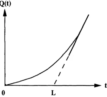
the solid, while the other side is evacuated. The buildup of gas on the evacuated side is measured as a function of the time, t. After decay of transients, the amount of gas accumulated, Q(t), per unit area of the solid follows the law,
Q(t) = A(t - L) (1)
where the intercept, L, on the f-axis is called the time-lag and gives the method its name. Figure 1 illustrates the relationship between Q(t) and its long-time asymptote given by Eq. (1).
The theory of Q(t), which is based upon solution of Fick's second law, provides expressions for L and the slope, A.1'2 When these are combined with the
experimental measurements of Q(t) vs t, the diffusion coefficient and other properties of the gas-solid system can be evaluated. The method has proved to be applica-ble to a number of proapplica-blems, including diffusion of gases through metals,3"9 polymers,11^16 oxide films,17 rocks,18
and zeolites.19
In some cases, the solids are not inert but in-stead actively evolve various gases. Examples include
a'Also with the University of Alabama System Ph.D. Program in
Materials Science.
Q(t)
t
- • t
0
FIG. 1. Dependence of the amount of accumulated gas, Q(t), upon time, t. The solid curve is Q(t) vs t for all t, while the dashed line represents the long-time asymptote, Q(t) = A(t — L), having slope, A, and time-lag, L.
radioactive decay of minerals to form a gaseous daugh-ter (emanation),20 rejection of plasticizer from polymer
films,13 and the decomposition of solid rocket propellants
in storage. Solid propellants are especially interesting be-cause, as complex mixtures, they are capable of evolving more than one gas.
Below, we develop the time-lag method for the diffusion of a gas through a planar sheet of solid, which is simultaneously evolving the same gas. We also give a J. Mater. Res., Vol. 8, No. 6, Jun 1993 © 1993 Materials Research Society 1455
formula for the rate of evolution of a gas from the sheet upon passive standing. The latter is useful in assessing the shelf life of the propellant.
II. INTEGRATION OF FICK'S SECOND LAW
A. Conversion to an ordinary differential equation
Consider a slab of thickness, h, in the x-direction. In order to ignore edge effects, the slab will be considered to be infinite in both directions perpendicular to its thickness. The instantaneous concentration of gas at position x within the slab is c(x, t).
In the case of active gas evolution, Fick's second law takes the form
dc(x,t) nd2c(x,t)
dt dx2 0 h (2)
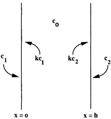
where D is the coefficient of gas diffusion through the solid and f(t) is the volume rate of internal gas production, which is assumed to be spatially uniform. The gas just outside the face at x = 0 has the concentration, c\. The gas concentration associated with the solid just inside the face is kc\, where k is the thermodynamic distribution coefficient. On the face at
x = h, the analogous concentrations are c2 and kc2,
respectively. At t = 0, the bulk solid contains gas at concentration, c0, which, depending upon the immediate
past history of the solid, can be equal to or different from the thermodynamic solubility of the gas. These statements, illustrated in Fig. 2, are summarized by the equations, c(x, 0) = c0 c(0, t) = ka c(h, t) = kc2 (3) (4) (5) Equations (2)-(5) define a boundary value prob-lem for the function, c(x, t). The probprob-lem is readily solved by introducing the Laplace transform,21 which
for an arbitrary function, w(t), we denote as L[w(?)] =
w(s), where
00
w(s) = I dt exp(-st)w(t) (6)
Forming the Laplace integrals of Eqs. (2), (4), and (5) gives
cxx(x,s) - (s/D)c(x,s) = -(co/D) - f{s)/D (7)
c(0,s) = kci/s (8)
c(h,s) = kc2/s (9)
where in Eq. (7) cxx(x, s) = d2c(x, s)/dx2, and we have used the theorem, L[c(x, t)] = sc(x,s) — c0.22
Equation (7) is an ordinary differential equation in x with boundary conditions specified by Eqs. (8)
kc
r
J
x = o x = h
FIG. 2. Solid slab illustrating the initial and boundary conditions applying to the gas concentration.
and (9). Since the right-hand side of Eq. (6) is inde-pendent of x, it can be integrated most easily by the operator method23 to obtain
c{x, s) = (c2
-- co)
s i n h
[ ^ - *)]
sinh Jjf l v D X sinh sinh U/nO -
x) j
a - A , ,
sinh [J |jx s sinhinh(^) (10)B. Inversion to the time domain
To invert c(x,s) to obtain c{x, t), we need the integral,
c(x,t) = -^ [ dsc(x,s) exp(sr) (11)
2TTI Jwhere a > 0 and i = (-1)1'2.2 1 The evaluation of
Eq. (11) proceeds by way of the residue theorem,24 for
which purpose we catalog the analytic properties of the following complex valued functions:
(i) Analytic properties of the function, s"1 exp(st) X sinhU(s/D) x]/ swh[y/(s/D) ti\. Despite the -Js
which appears in the arguments of the hyperbolic sines, their ratio is single valued in the vicinity of s = 0. For small s, the function approaches (x/hs) exp (st), which has only a simple pole. The residue at 5 = 0 is
res(0) = x/h, 0 (12)
An infinite sequence of poles is associated with the zeros of sinh[*J (s/D)h]. These occur along the real axis in the left half-plane at the points, sn = -n2v2/Dh2, where n ~ss 1 is an integer. The residue associated with one of
these poles is
HTT sin exp
-n27r2t
Dh2
(13) (ii) Analytic properties of the function, s 1 exp(st)
X sinh[V<>/£>)(/i - x)]/sinh[^(s/D)h]. The poles of this function are the same as those listed above. The residue at s = 0, however, is
res(O) = (h - x)/h, t 3= 0 while the residues at sn = —n2/n2/Dh2 are
(14)
nir sin
fnw(h -x)\ (~n27T2t
\ h exp Dh2
(15) (iii) Analytic properties of the function s 1 exp(sf).
This function has a simple pole at s = 0, where the resi-due is
res(0) = 1 0 (16)
After substituting Eq. (10) into Eq. (11) and evaluating the integral using the Bromwhich contour,21
we find - kc2(-iy - kCl
. f
X sin V . Innx V h exp -n2TT2Dt\ h2 J 4_£o 77 X X X exp (2m + \)TTX \2m + 1/ L h -(2m + \)2TT2D(t - t1) h2 (17)To obtain Eq. (17), we have used the identity,
sm[rnr(h - x)/h] = - ( - 1 ) " sin(rnrx/h), and the fact
that 1 — (—1)" is zero when n is even and 2 when n is odd. The integral in Eq. (17) follows by application of the convolution theorem to the term involving f(s) in Eq. (10).21 Equation (17) is the general solution for c(x, t) from which our subsequent results follow.
III. RATE OF OUTGASSING
The flux of gas molecules in the x -direction at any point within the slab is given by Fick's first law,
J(x, t) = -Ddc(x, t)
dx (18)
The sum of the fluxes exiting both sides of the slab is
= -J(P,t) + J(h,t) (19)
where the minus sign accounts for the fact that the positive x-axis runs from x = 0 to x = h.
In the case of a slab of solid propellant under shelf storage conditions, it is likely that the steady state concentrations of gas on either face will be zero or close to it. The concentration of gas anywhere within the slab is then given by settling c\ = c2 = 0 in Eq. (17). By
combining Eqs. (17)-(19), one obtains
to =
8£>J
Co ? expI
m=0 -(2m + \)2TT2Dt h2 -(2m + l)2TT2D(t - t') h2 (20)For times t > h2/TT2D, the terms proportional to c0 in
Eq. (20) will be small, and Jt0( takes on the
asymp-totic form /tot(0 =
— / dt'fW) 2, exp
h o m = 0 -(2m + l)lTT2D(t - t') h2 (21)IV. TIME-LAG METHOD
A. Cumulative mass transported
If the gas concentration on the high pressure side at
x — h is C2, while on the low pressure side at x = 0 it
is c\, then the cumulative amount of gas passed through the slab after a time, t, is
After substituting Eq. (17) into Eq. (18) and the resulting equation into Eq. (22), we obtain
Dk(c
2- g)t (2h\\ f fc[(-l)"c
2~ c{\
h W
2)\
X [1 - exp(-n27r2Dt/h2)]\ V 772 J^0(2m + I)2 X {l - exp[-(2m + l)2772Df/ft2]}'
4
£)z/W*w>
- t')/h2] (23) (24) X exp[-(2m + 1) If we define a2 = (2m + \)2TT2D/h2the double integral in Eq. (23) can be rewritten as
/ = f dt" f dt'f(t') cx
V[-a
2(t" - t
1)] (25)
0 0
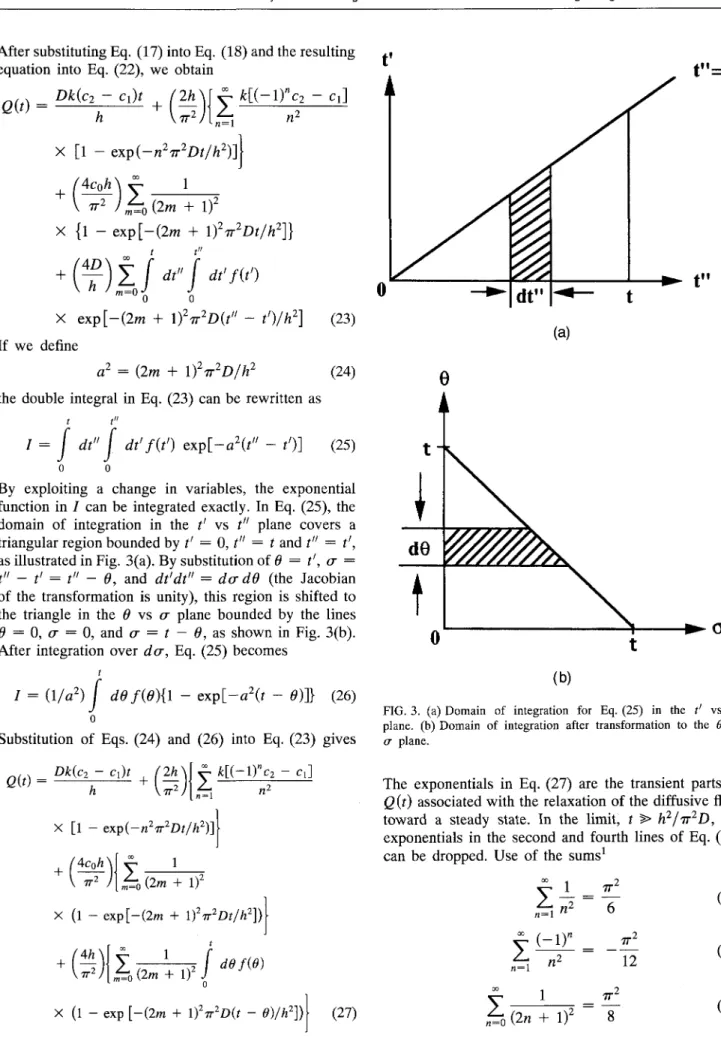
By exploiting a change in variables, the exponential function in / can be integrated exactly. In Eq. (25), the domain of integration in the t' vs t" plane covers a triangular region bounded by /' = 0, t" = t and t" = t', as illustrated in Fig. 3(a). By substitution of 6 = t', a = t" - t1 = t" - 6, and dt'dt" = da dO (the Jacobian of the transformation is unity), this region is shifted to the triangle in the 6 vs a plane bounded by the lines
0 = 0, u = 0, and a = t — 6, as shown in Fig. 3(b).
After integration over da, Eq. (25) becomes t
I = (I/a
2) f ddf{6){\ - exp[-a
2(f - 0)]}
(26) Substitution of Eqs. (24) and (26) into Eq. (23) gives. X [1 - exp(-n2iT2Dt/h2)] 1 X 7T
f
i(2m+ I)2 - exp[-(2m + l) X (1 - exp [-(2m + lfw2D(t - 9)/h2])\ (27)(a)
t"=f
t"
(b)FIG. 3. (a) Domain of integration for Eq. (25) in the t' vs t" plane, (b) Domain of integration after transformation to the 9 vs a plane.
The exponentials in Eq. (27) are the transient parts of
Q(t) associated with the relaxation of the diffusive flow
toward a steady state. In the limit, t > h2/7T2D, the exponentials in the second and fourth lines of Eq. (27) can be dropped. Use of the sums1
77
Y (-1)"
EL
n=\ 00 1y—-n=0 (2/1 + 77 (28) (29) (30)
then allows us to compute the limiting form for the mass transported: Q{f) ^ X \ t -c2 X (1 - exp[-(2m + l)27T2D(t - 6)/h2])\ (31) The first term in Eq. (31) has the standard form of the time-lag law expressed by Eq. (1). The sum of integrals involving f(6), however, is more complex. Depending upon the form of f(0), this sum may contribute to either or both of the constants in Eq. (1); it may even introduce terms that are nonlinear in t, so that Eq. (1) fails to apply at all.
B. Constant rate of gas evolution
In the special case that the rate of gas evolution is independent of time,
fit) = R
(32)where R is a constant. Substitution of Eq. (32) into Eq. (31) followed by use of the condition t > h2/TT2D and the sum25
1 f=-0(2m + l)4 77 96 (33) yields, hR\ 1 r . , h3R~\ (34) where we have also set ci = 0 as is customary in the case of time-lag experiments.
Equation (34) has the general time-lag form given by Eq. (1). By comparison of these two equations, one may write
hA = Dkc2 + h2R/2 (35)
AL/h = kc2/6 + h2R/24D - co/2 (36) Experimental data involving Q(t) vs t can be fit to Eq. (34) by treating hA and AL/h as least squares adjustable parameters.
V. DISCUSSION
A. Analysis of experimental data
Equations (35) and (36) have been left in forms convenient for the analysis of experimental data so as to obtain values for D, k, R, and c0. If it is assumed
that h is directly measurable, then a plot of hA vs c2 as shown in Fig. 4(a) should form a straight line with slope,
Dk, and intercept, h2R/2. From the value of h and the intercept, R can be obtained. By comparison, a plot of
AL/h vs c2 as shown in Fig. 4(b) should form a straight line with slope k/6 and intercept (h2R/24D - cj2).
The slope of this line determines k directly, and when combined with the value of Dk, the value of D can be computed. Once D and .ft are determined, the value of c0 can be obtained from the value of (h2R/24D — cj2).
B. Calculation of A and L from Q(s)
Under certain conditions, it is possible to make theoretical calculations of A and L in Eq. (1) without the effort of direct inversion of c(x, s) to the time domain as
hA
Dk
(a)
AL/h
24D 2,
0
(b)was done in Sec. II. B. In cases where direct inversion is unnecessary,26 the Laplace transforms,
and
J(x,s) = — Dcx(x, s)
Q(s)= -J(0,s)/s
(37)
(38) of Eqs. (18) and (22), respectively, can be combined with
c{x,s) to obtainQ(s) in the general form,
(39)
Q(s) = A ( \ - - ) + Z(s)
The function Z(s) accounts for the transient terms in
Q(t) and has the properties,
and lim s2Z(s) = 0 O lim — [s2Z(s)] = 0 (40) (41) Given Eqs. (40) and (41), A and L can be computed from Eq. (39) as the limits,
A = lim [s2Q{sj\
s->0
and
(42)
(43)
respectively. In the important special case where an active solid outgasses exponentially with time at the spe-cific rate A, so that f(t) = const. X exp(-Xt) [f(s) = const./(,s + A)], this procedure is possible.
For arbitrary f(t), however, resorting to the time domain is necessary. For this reason (plus the fact that the singularities of c(x,s) given by Eq. (10) permit it to be readily inverted), we have chosen to obtain the explicit form of c(x, t) and use Eqs. (17), (18), and (22) to compute Q(t).
C. Hydrogen trapping in metals
lino4 has provided a time-lag theory for the problem
of hydrogen trapping in metals, in which H atoms diffusing through a metal are assumed to undergo the homogeneous, reversible reaction,
H + S ^ HS
where S is an empty site and HS is an occupied site. To preserve the linearity of Fick's second law, lino treats the case where the concentration of trapping sites is in vast excess over that of the diffusing H atoms. In this circumstance, the rate law for the forward reaction becomes zeroth order in S and first order in H while the rate law for the reverse reaction is first order in HS.
The theory we have presented above ignores the details of the chemical kinetics associated with the solid and the dissolved gas by representing them by the general function /(?)• This would seem to be appropriate in the case of rocket propellants, for example, where the mechanism of gas evolution is not yet understood.
D. Summary
Equations (21), (27), and (34) have been written with the case of a single diffusing gas in mind. If more than one species is being considered, then subscripts, "i", running over the number of species need to be appended to the symbols D, k, c\, c2, c0, f(t), J\oi{t), and Q(t). When it is then required to compute the total gas
evolution by including the effects of all species involved, the appropriate equation selected from Eqs. (21), (27), (31), and (34) need only be summed over "/" to get the desired result.
Equations (17) and (27) have appeared previously for the special case f(t) = 0.27 The present work
gener-alizes these equations to an outgassing solid [f(t) J= 0]. The specific new results are summarized by Eqs. (17), (20), (21), (27), (31), and (34). Once D has been determined in a time-lag experiment as described above, Eqs. (20) and (21) (as applicable) can be used to predict the rate of gas evolution per unit area of an active solid. These formulas should have special utility in predicting the shelf life of solid rocket propellants.
ACKNOWLEDGMENTS
The participation of J. K. Baird in this research was sponsored by the Morton Thiokol Corporation and by the National Aeronautics and Space Administration through contract NAGW-812 with the Consortium for Materials Development in Space at the University of Alabama in Huntsville. The participation of J. S. Chen was sponsored by the National Science Council of Taiwan, Republic of China, under project NSC 82-0208-M-009-019.
REFERENCES
1. W. Jost, Diffusion in Solids, Liquids, and Gases (Academic Press, New York, 1960), p. 44.
2. J. Crank, The Mathematics of Diffusion (Oxford University Press, London, 1957), p. 48.
3. J. McBreen, L. Nains, and W. Beck, J. Electrochem. Soc. 113, 1218 (1966).
4. M. lino, Acta Metall. 30, 367 (1982).
5. T. N. Kompaniets and A. A. Kurdyumov, Prog. Surf. Sci. 17, 79 (1984).
6. A. S. Schmidt, F. Verfuss, and E. Wicke, J. Nucl. Mater. 131, 247 (1985).
7. R. Nishimura, R.M. Latanision, and G. K. Hukler, Mater. Sci. Eng. 90, 243 (1987).
8. S. K. Yen and H. C. Shih, J. Electrochem. Soc. 137, 2028 (1990). 9. R.N. Iyer and H.W. Pickering, Ann. Rev. Mater. Sci. 20, 299
10. J. S. McBride, T. A. Massaro, and S. L. Cooper, J. Appl. Polym. Sci. 23, 201 (1979).
11. J. Springer and H. Brito, J. Appl. Polym. Sci. 24, 329 (1979). 12. S.J. Napp, W. Huang, and M. Yang, J. Appl. Polym. Sci. 28,
2793 (1983).
13. I.R. Bellobono, B. Marcandalli, E. Selli, and A. Polissi, J. Appl. Polym. Sci. 29, 3185 (1984).
14. K. Schaupert, D. Albrecht, P. Armbruster, and R. Spohr, Appl. Phys. A 44, 347 (1987).
15. M.M. Alger and T.J. Stanley, J. Appl. Polym. Sci. 36, 1501 (1988).
16. A. Higuchi and T. Nakagawa, J. Appl. Polym. Sci. 37, 2181 (1989).
17. E.A. Irene, J. Electrochem. Soc. 129, 413 (1982).
18. H. Meier, E. Zummerhackl, W. Hecker, G. Zeitler, and P. Menge, Radiochem. Acta 44-45, 239 (1988).
19. Ref. 1, pp. 300-304. 20. Ref. 1, pp. 314-319.
21. G. Arfken, Mathematical Methods for Physicists (Academic Press, New York, 1985), pp. 824-859.
22. Ref. 21, p. 831.
23. See, for example, A. L. Nelson, K. W. Folley, and M. Coral, Differential Equations, 2nd ed. (D. C. Heath and Co., Boston, MA, 1960), pp. 97-99.
24. Ref. 21, p. 400.
25. I. S. Gradshteyn and I. M. Ryzhik, Table of Integrals, Series, and Products (Academic Press, New York, 1980), p. 7, formula 0.234.5.
26. J. S. Chen and F. Rosenberger, J. Phys. Chem. 95, 10164 (1991). 27. H. Daynes, Proc. R. Soc. London A 97, 286 (1920).