A Spatial-Extended Background Model for
Moving Blobs Extraction in Indoor Environments
*SAN-LUNG ZHAOAND HSI-JIAN LEE+
Department of Computer Science National Chiao Tung University
Hsinchu, 300 Taiwan E-mail: slzhao@csie.nctu.edu.tw
+
Department of Medical Informatics Tzu Chi University Hualien, 970 Taiwan E-mail: hjlee@mail.tcu.edu.tw
This paper presents a system for extracting regions of moving objects from an image sequence. To segment the foreground regions of ego-motion objects, we create a back-ground model and update it using recent backback-ground variations. Since backback-ground images are usually changed in blobs, spatial relations are used to represent background appear-ances, which may be affected drastically by illumination changes and background object motion. To model the spatial relations, the joint colors of each pixel-pair are modeled as a mixture of Gaussian (MoG) distributions. Since modeling the colors of all pixel-pairs is expensive, the colors of pixel-pairs in a short distance are modeled. The pixel-pairs with higher mutual information are selected to represent the spatial relations in the background model. Experimental results show that the proposed method can efficiently detect the moving object regions when the background scene changes or the object moves around a region. By comparing with Gaussian background model and the MoG-based model, the proposed method can extract object regions more completely.
Keywords: background modeling, background subtraction, object segmentation, video
surveillance, mixture of Gaussian
1. INTRODUCTION
Human extraction is important in indoor surveillance systems for visual-based pa-tient-caring, security-guarding, etc. In an indoor environment, people are usually consid-ered to be the only foreground objects, which are defined as ego-motion objects. If the images with only background objects can be captured in advance, the positions of fore-ground objects can be detected by comparing the current image with the backfore-ground im- ages. However, background images vary when camera positions, background object po-sitions, and illuminations change. Tracking objects in general environments will become very complicated.
In many surveillance applications especially in indoor environments, camera po-sitions are generally fixed. Illumination variations and background object motion may
Received December 12, 2007; revised April 21, 2008; accepted May 8, 2008. Communicated by H. Y. Mark Liao.
* This work was supported in part by the Ministry of Economic Affairs (MOEA), Taiwan, R.O.C., under grant
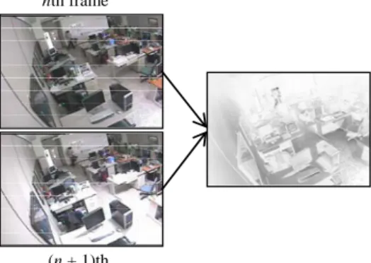
Sci-change the captured images significantly. Examples of the motions include placing a book on a desk and moving a chair to another position. The positions of the objects are usually changed by people or other external forces. After the motion stops, these objects remain in the same position for a certain period; these motions are usually not repeated. In an indoor environment, the illumination of objects is not affected by continuous light changes, such as sun rise, sun set, or weather changes. Ignoring these continuous changes, brightness variations such as turning lights on or off, as shown in Fig. 1, and opening a window are assumed to be abrupt. Several researchers [2] assumed that brightness varia-tions due to illumination changes are uniform. The right-hand side image in Fig. 1 shows the intensity differences after the lights were turned on. We observe that brightness varia-tions in different pixels are not uniform. It is difficult to process this kind of variavaria-tions. Several other researchers [2, 4, 5, 8] assumed that illumination changes are not repeated like the motion of freely movable objects. However, light sources can be repeatedly turned on or off several times over a period of time. The appearance changes on the illu-minated regions will also be repeated.
(n + 1)th nth frame
Fig. 1. Left column: two consecutive images in different illumination conditions. Right image: intensity differences between the left two images.
To model the non-repeated background changes, we can use an online updating scheme to adapt to the background appearances in recently captured images [1-17]. When the appearances of a pixel repeatedly change, they can be modeled as a Mixture of Guas-sians (MoG) [9]. The online updating MoG model is useful for modeling rapidly re-peated background appearances such as waves on water surface, but does not works well in long-term repeated appearances such as door opening and closing. In consecutive im-ages, the repeated appearances of background objects usually appear in blobs in fixed places, while the appearances of foreground objects usually change their places and do not form fixed blobs. In this study, we extend the MoG model by using the spatial rela-tions among pixels to model the background appearances.
The objective of our system is to extract moving object from a sequence of images. The system is divided into two modules: background modeling and foreground detection. The first module creates a background model to represent possible background appear-ances. The parameters of the model are learned and updated automatically from recently captured images. In the background model, the distributions of background features are
assumed to be mixtures of Gaussians [9]. Since background appearances are changed in blobs, the features used in the MoG should be able to represent spatial relations in the blobs. To represent the spatial relations, we estimate the joint color distributions of pixel- pairs in a short distance. Since estimating the distributions of all pixel-pairs is costly and not all pixel-pairs provide enough information to model background, we first calculate the dependence of colors in each pixel-pair. A pixel-pair with a higher color dependence implies that the two pixels provide more information to represent the appearance changes in blobs. Highly dependent pixel-pairs are then selected to model the spatial relation of background. In the second module, the background model that has already been updated from recent images is used to calculate the background probability of each pixel of the current image. The probability is then used to decide whether the pixel belongs to the foreground or background. Connected foreground pixels are extracted to form foreground regions.
The remainder of this paper is organized as follows. In section 2, we review related work on training methods of background models. In section 3, we describe the spa-tial-extended background model using the colors of pixel-pairs. In section 4, we design an algorithm to find the pixel-pairs that can provide more information to model spatial dependency. In section 5, we test the effectiveness of the background model in video clips and analyze the experimental results. In section 6, we conclude this paper.
2. RELATED WORK AND ISSUES IN BACKGROUND MODELING
A background model in a surveillance system represents background objects. The method that compares the current processed image with the background representation to determine foreground regions is called background subtraction. If the background is unchanged but affected by Gaussian noise, the colors of the background pixels can be modeled as a Gaussian distribution with mean vector (μ) and covariance matrix (∑) [1-8]. Background subtraction is then performed by calculating the probability of each pixel in the current image belonging to the Gaussian model.
Since background appearances may be affected by external forces, modeling a pixel with a Gaussian distribution may misclassify some background pixels as foreground ones. In many cases, the background may change repeatedly. A background pixel with repeated changes can be divided into several background constituents and modeled as an MoG distribution [9-13]. For each background constituent in a pixel, the means (μi), covari-
ances (
∑
i), and weights (wi) of the ith constituent (bi) have to be estimated. If there areK background constituents, the parameters of the background model can be represented as {μi,
∑
i, wi |1 ≤ i ≤ K}. In order to decide whether a sample point X belongs to thebackground B, the conditional probability P(B|X) is calculated as follows:
1 1 ( | ) ( | ) ( ; , ), K K i i i i i i i P B X w P b X wη X μ = = =
∑
∝∑
Σ
(1) where η represents a Gaussian probability density function,1 1 2 1 2 2 ( ) ( ) 1 ( ; , ) . (2 ) | | T i i i n X X i i i X e μ μ η μ π − − − ∑ − =
Σ
Σ
(2)The motion of some background objects may not be repeated. After the motion, the objects remain in the same position for a period. To model the background changes, re-searchers have proposed methods for online updating of the parameters of background models [1-17]. The mean vector and covariance matrix in time t are represented as μt and
∑
t, respectively. The updating rules are formulated as follows:μt = (1 − ρ)μt-1 + ρXt, (3)
∑
t = (1 − ρ)∑
t-1 + ρ(Xt − μt)(Xt − μt)T, (4)where ρ is used to control the updating rate. To integrate the updating method into an MoG model, Stauffer and Grimson [9] proposed a method to update the mean vector and covariance matrix of a background constituent to match those of Xt in Eqs. (3) and (4).
The weight wi,t of the ith background constituent is updated as follows:
wi,t = (1 − α)wi,t-1 + αIi,t, (5)
where Ii,t is an indicator function, whose value is one if the ith background constituent
matches Xt and zero otherwise, and α is a constant used to control the updating rate of the
weights. In Stauffer and Grimson’s method [9], the updating rate ρ for the parameters of the ith constituent (Gaussian distribution) is calculated according to α and η(X; μi,
∑
i).To make background models more robust, researchers tried to modify updating rules or adopt different features [10-13]. In adaptive background models, background objects are assumed to appear more frequently than foreground ones. However, the assumption is not always satisfied. If the appearances of a background pixel appear less frequently than those of foreground objects, the background pixel is probably misclassified as a foreground object. Taking the following case as an example, assume a room is monitored by a fixed camera and the background objects in the room include a door and a wall as shown in Fig. 2 (a). People may enter the room, and close or open the door. If a person
door
knob
(a)
person
(t + 1)th frame (t + 2)th frame (t + 30)th frame clothes
(b)
Fig. 2. (a) Sketches of two possible background scenes. Left: door closed; Right: door opened. (b) Consecutive frames of a person moving from left to right.
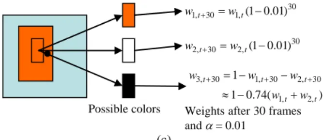
Possible colors Weights after 30 frames andα= 0.01 30 1,t 30 1,t(1 0.01) w + =w − 30 2,t 30 2,t(1 0.01) w + =w − 3, 30 1, 30 2, 30 1, 2, 1 1 0.74( ) t t t t t w w w w w + = − + − + ≈ − + (c)
Fig. 2. (c) Possible colors and their weights of the rectangle region shown in the left image.
(a) Scene when the door is closed. (b) Scene when the door is opened.
Fig. 3. Sketches of a person whose clothes colors are similar to the door color in front of different background scenes.
wears a suit of clothes of single color and walks slowly across the room as shown in Fig. 2 (b), the major color of the clothes may be captured repeatedly in a certain position among several consecutive images. Assume that the person moves from left to right in 30 frames. If the updating rate α in Eq. (5) is set as 0.01, the weight of the repeatedly cap-tured color of the clothes in the images will increase from 0 to 0.26, as shown in Fig. 2 (c). This large weight may cause the clothes to be labeled as the background, when the MoG model in Eq. (1) is used. Using a small updating rate can overcome this problem; however, the background model will be updated very slowly and may fail to learn back-ground changes.
In another situation, the color of the person’s clothes is assumed to be the same as that of the door, as illustrated in Fig. 3 (a). If the person enters the room and passes through the door, the region of clothes may be labeled as background due to the similar-ity of colors. However, after the door is opened, the current background color is not simi-lar to the clothes color as shown in Fig. 3 (b). The clothes may still be labeled as the background, since they are very similar to possible background colors been estimated.
In these two situations, we observe that modeling each pixel independently cannot sufficiently represent the similarity among different object appearances caused by either object motion or illumination changes. Most researchers regarded the variations caused by object motion as foreground changes and attempted to eliminate the effect caused by illumination. In consecutive images, when the illumination changes, the pixels of an ob-ject are usually changed simultaneously. In order to model background obob-jects, the pixels at different positions should be considered together. To represent the relation among the pixels, Durucan and Ebrahimi [14] proposed to model the colors of a region as vectors.
They segmented the foreground regions by calculating the linear dependence between the vectors of the current image and those of the background model. However, it is ex-pensive to represent the dependence between vectors in terms of storage and speed. To reduce the cost, the vector of a region should be reduced to a lower dimensional feature. Li et al. [15, 16] used two-dimensional gradient vectors as the features of local spatial relations among neighboring pixels. In their proposed method, the appearance variations caused by illumination changes can be distinguished from object motion. However, the gradient features cannot be used to extract the foreground region that has a uniform color. To model the relation among pixels, we need to use the relations among near pixels to reduce time and storage consumption, and then extend the relations into a more global form.
The methods based on the Markov random field (MRF) are well known for extend-ing the neighborextend-ing relations among pixels into a more global form. Image segmentation methods based on MRF [17, 19] assume that most pixels belonging to the same object have the same label and these pixels form a group in an image. The MRF combines col-ors among a clique of pixels in a neighboring system and uses an energy function to measure the color consistency. Then, the maximum a posterior estimation method is used to minimize the energy for all the cliques to find the optimal labels. In the MRF-based methods, the final segmentation results are strongly dependent on the energy functions of the labels in different cliques. If a high energy is assigned to the clique with unique la-bels, the extracted foreground regions will become more complete than those of the pixel-wise background models. An additional noise removal process is not required. However, when several pixels are mis-labeled, these errors will propagate into neighbor- ing pixels. The error propagation will cause more pixels to be mis-labeled. In this re-search, we directly estimate the relations among pixels instead of the labels, and there-fore the errors will not easily propagate.
3. JOINT BACKGROUND MODEL
In a sequence of images, colors will change in blobs instead of individual pixels due to illumination changes or object motion. This paper proposes to utilize the relations among pixels to represent the changes in blobs. The relations are formulated as a spatial- extended background model, which is then used to classify the pixels into either fore-ground or backfore-ground.
3.1 Spatial Relation in Images
Using pixel-wise features, if the color of a foreground pixel is similar to those of the background, the pixel may be misclassified as background. If we can estimate the distri-butions of color combinations for the pixels in blobs, the foreground objects can be clas-sified more precisely. Suppose there is a red door in a room and the appearance outside the door is white. When a person wearing a suit of interlaced red and white stripes passes through the door, parts of the suit may be misclassified as background when the colors of the pixels are modeled independently. Nevertheless, if we model the background appear- ances among pixels using joint multi-variate color distributions, the interlaced red and
white stripes can be classified as foreground using the method introduced later. However, estimating the multi-variate distributions for all pixel-pairs is still costly since the num-ber of pixel combinations may be very large. In this research, we will estimate the color distributions of joint random vectors in closed pixel-pairs.
As stated in section 1, illumination changes and background object motions may change background appearances. Since the changes are complex, it is difficult to collect enough training samples for all the possible changes. In this paper, we modify Eq. (4) for updating the color distributions of pixel-pairs to adapt to the appearances that have not been trained, to be described in section 3.3.
3.2 Calculation of Background Probabilities
Assume that we have already estimated the color distributions of all background pixel-pairs. In this research, we decide whether pixel a1 belongs to foreground according to its color and the color combinations of pixel-pairs (a1, A), where A denotes a set of pixels associated with a1.
Suppose that a sequence of pixels (a0, a1, …, an) has a corresponding color
se-quence (c0, c1, …, cn). The probability of pixel a0 belonging to background can be repre-sented as P(B0 |x0 = c0, x1 = c1, …, xn = cn), where the sequence (x0, x1, …, xn) denotes the
joint random variable of the colors for the sequence (a0, a1, …, an), and B0 represents the event that pixel a0 belongs to the background. Assuming that x1, x2, …, xn are
condition-ally independent, based on the naive Bayes’ rule, the probability P(B0 |x0 = c0, x1 = c1, …, xn = cn) can be computed as the product of n pair-wise probabilities:
0 0 0 1 1 0 0 0 0 0 1 ( | , , ..., ) ( | ) ( , ). n n n i i i P B x c x c x c P B x c P x c x c = = = = ≈ =
∏
= = (6)When estimating the background probabilities from above equation, we face two problems. The first one is the estimation and updating of the probability distributions P(B0 |x0), P(x0, xi), and P(xi). The distribution P(B0 |x0), a pixel-wise background color distribution, is regarded as an MoG and can be calculated from Eq. (1), whose parame-ters are estimated and updated by using Eqs. (3)-(5). It is tedious to estimate and update the bivariate probability distribution P(x0, xi), since the number of possible color
combi-nations in x0 and xi is large. We will simplify the estimation and updating by combining
the MoGs of pixels to form the joint random vector distributions of pixel-pairs. The sec-ond problem is the cost of modeling pixel-pairs. To model all pixel-pairs, the number of pixel-pairs is O(W2 × H2), where W and H are the width and height of the images, re-spectively. We reduce the complexity by only modeling the pixel-pairs that can provide sufficient information to represent spatial relations as described in section 4.
3.3 Estimation of Bivariate Color Distributions
As mentioned before, the color distributions of pixel-pairs should be updated to adapt to the background changes. If we assume the color distributions in a pixel-pair (a1, a2) to be independent, the joint probability P(x1, x2) can be regarded as P(x1) ⋅ P(x2). As-suming the color distributions are a mixture of Gaussians, the background colors of the
two pixels a1 and a2 form several background constituents, which can be represented as Gaussian distributions G1 = {η(μk1,
∑
k1)|1 ≤ k1 ≤ K1} and G2 = {η(μk2,∑
k2)|1 ≤ k2 ≤ K2}, respectively. The weights in both distributions are denoted as W1 = {wk1 |1 ≤ k1 ≤ K1} and W2 = {wk2 |1 ≤ k2 ≤ K2}. When the independence is satisfied, the joint color of the pixel pair (a1, a2) forms K1 × K2 background joint constituents, and the joint color distributions of the constituents are combinations of G1 and G2, denoted as G = {η(μk1,k2,∑
k1,k2)|1 ≤ k1 ≤ K1,1 ≤ k2 ≤ K2, μk1,k2 = (μk1, μk2),∑
k1,k2 is the covariance matrix}. The weights of the joint constituents are W = {wk1 ⋅ wk2 |1 ≤ k1 ≤ K1, 1 ≤ k2 ≤ K2}. Since the parameters of G1 and G2 can be estimated from Eqs. (3) and (4), the parameters (G, W) of the bi-variate MoG P(x1, x2) can be calculated easily.In our background model, since the dependence between the colors of two pixels is used to model the spatial relations, the colors cannot be assumed independent. To esti-mate the parameter of a bi-variate MoG P(x1, x2), we first examine the example depicted in Fig. 4. This figure shows the colors of three pixels a1, a2, and a3 collected from 1,000 consecutive images, where a1 and a2 belong to the same object but a3 does not. The
a1 0 50 100 150 200 250 300 1 72143 214 285 356 427 498 569 640 711 782 853 924 995 R G B 0 50 100 150 200 250 300 1 72143 214 285 356 427 498 569 640 711 782 853 924 995 R G B 0 50 100 150 200 250 300 1 73145 217 289 361 433 505 577 649 721 793 865 937 R G B a2 a3
(a) A sample image and the colors in three pixels in a time period.
0 50 100 150 200 250 x40.80 0 50 100 150 200 250 x3 0.7 0 r(x1) r(x3) r(x2) 0 50 100 150 200 250 x40.80 0 50 100 150 200 250 x50. 90 0 5 0 1 0 0 1 5 0 2 0 0 2 5 0 x 4 0 . 8 0 0 . 0 0 0 0 . 0 0 5 0 . 0 1 0 0 . 0 1 5 0 . 0 2 0 R1 R2 R3 R4
(b) Scatter plots of the pixels in the spaces (r(x2), r(x3)) and (r(x2), r(x1)), and probability distribu-tions of r(x1), r(x2), and r(x3).
right-hand side image of Fig. 4 (a) shows the histograms of the colors in a1, a2, and a3 in a time period of the sample image in the left. From the histograms, we observe that the colors of a1 and a2 usually change simultaneously and their values are dependent. The two scatter plots of Fig. 4 (b) from top to bottom are the scatters of (r(x2), r(x3)) and (r(x2), r(x1)), where r(xi) denote the red values of the color random variable xi. The projection
profiles from the top to bottom are the probability distributions of r(x3), r(x1), and r(x2). Each probability distribution forms several clusters and each cluster is regarded as a background constituent. As shown in the scatter plots, several combinations of back-ground constituents in a pixel-pair form joint backback-ground constituents. When the prob-ability distributions of a pixel-pair (a1, a2) are regarded as bi-variate MoGs, the probabil-ity function P(x1, x2) is formulated as follows:
1 2 1 2 1 2 1 2 1 2 1 1 2 2 , 1, 2 , , 1 1 ( , ) ( , , ). K K k k k k k k k k P x c x c w η c μ = = = = =
∑ ∑
⋅∑
(7) In the equation, the color vector c1,2 is the joint color vector of colors c1 and c2, and the mean μk1,k2is the vector [μk1, μk2], where μk1 and μk2 can be estimated from the background updating in Eq. (3). The covariance matrix∑
k1,k2 is estimated with respect to the mean μk1,k2 as 1 2 1 2 1 2 1 2 1 2 1 2 ( 1) , (1 , (1, 2)) , , ( 1, 2)(1, 2 , )(1, 2 , ) , t t t t t t t t T k k αk k c k k αk k c c μk k c μk k − = − + − −∑
∑
(8) where the 1, 2 t c and 1, 2 t k kμ are the joint color vector and joint mean vector in the pixel-pair (x1, x2), respectively. In the equation, if a joint vector of colors is matched with a joint constituent, the covariance matrix of the joint constituent should be updated as follows:
1 2 1 2 1 2 1 2 1 2 1, 2 , , 1 2 1, 2 , , , 1, 2 if ( , , ) and , ( , ) argmin( ( , , )) ( ) , 0, otherwise t t t k k k k c t t t t k k k k k k dist c Th k k dist c c μ α μ α ⎧ < ⎪ ⎪ = = ⎨ ⎪ ⎪⎩
∑
∑
(9) where αc is a constant to control the updating rate, and ( 1, 2, 1, 2, 1,2)t t t
k k k k
dist c μ
∑
is a dis-tance function between the joint color vector 1, 2
t
c and joint mean vector
1, 2.
t k k
μ The proc- ess of determining the minimal distance
1 2 1 2
1, 2 , ,
( t , k kt , tk k )
dist c μ
∑
for all (k1, k2) is termeda matching process. In our experiments, the Mahalanobis distance is selected as the dis-tance function. If a joint color vector 1, 2
t
c does not match with any Gaussian distribution, a new Gaussian distribution is created and its mean is set as 1, 2.
t
c The weight of the new bi-variate distribution is initialized to zero.
The weight of a joint constituent in a pixel-pair is measured as the frequency of col-ors in the pixel-pair in past frames matched with the joint Gaussian distribution of the constituent, similar to Eq. (5). The updating rule of the weights is defined as
1 2 1 2 1 2 1 2 ( 1) , (1 , ( 1, 2)) , , ( 1, 2), t t t t k k k k k k k k w = −β c w − +β c (10) 1,2( 1, 2) ( ,1 1, 1) ( ,2 2, 2), t k k c c c k k c k k β =β η μ
∑
η μ∑
(11)where βc is a constant used to control the updating speed. Thus far, all the parameters
used for estimating the joint color probability in Eq. (7) are ready and the background probabilities of Eq. (6) can be estimated from a set of color joint probabilities in a set of pixel-pairs.
Note that, during the background model estimation, the weight wk1,k2 is not set as the product of wk1 and wk2. In other words, the constituents in the two pixels are not inde-pendent, and their relations are represented by the weights of the joint constituents. The relations in our model can be used to improve the accuracy of foreground detection. For example, in Fig. 4(b), the weight of joint constituents in R4 is approximately zero, since no pixels match with the constituents; that is, the two constituents belonging to pixels x1 and x2 in R4 usually do not appear simultaneously. However, when the joint colors in pixel-pair (x1, x2) match one of the joint constituents in R4, the pixel-pair (x1, x2) is classi-fied as foreground.
4. SPATIAL-DEPENDENT PIXEL-PAIRS SELECTION
The joint colors in pixel-pairs are used to represent the spatial relations of a back-ground model. In a scene, not all pixel-pairs contain sufficient spatial relations. Modeling the unrelated pixel-pairs is useless for foreground detection. To reduce the computation cost, we first find the pixel-pairs with higher dependence.
The colors of two pixels with high dependence will form compact clusters in the scatter plots as shown in Fig. 4 (b). The compactness of a bi-variate distribution is meas-ured from mutual information [20]. The mutual information I(xi, xj) for colors ci and cj is
defined as all in all in ( , ) ( , ) ( , ) log . ( ) ( ) i i j j i j i j i j c x i j c x P c c I x x P c c P c P c ⎛ ⎞ = ⎜⎜ ⎟⎟ ⎝ ⎠
∑
(12) Here, P(ci), P(cj), and P(ci, cj) can be computed from Eqs. (1) and (7). To reduce the costof calculating the probabilities for all possible colors, the probability P(ci, cj) can be
re-placed by the weights estimated from Eq. (10). The mutual information I(xi, xj) in Eq. (11)
can thus be reformulated as follows:
, , 1 1 , 1 1 , , 1 1 ( , ) log . j i j i j i K K K m n m n K m n i j m n K K m n m n m n n m w w I x x w w w ′′ ′′ ′′= ′′= = = ′ ′ ′= ′= ⎛ ⎛ ⎞⎞ ⎜ ⎜ ⎟⎟ ⎜ ⎜ ⎟⎟ ≈ ⎜ ⎜ ⎟⎟ ⎜ ⎜⎜ ⎟⎟⎟ ⎜ ⎝ ⎠⎟ ⎝ ⎠
∑ ∑
∑ ∑
∑
∑
(13)The pixel pair (xi, xj) with higher mutual information I(xi, xj) is selected to model spatial
relations of the background model.
5. EXPERIMENTAL RESULTS
by three different cameras. Two cameras are set in the two ends of a corridor (Cam1 and Cam2), and the other one is set in our laboratory (Cam3). The camera Cam1 is a gray-scale CCD camera, Cam2 a color CCD camera, and Cam3 a USB-Webcam. The resolu-tion of each video frame is 320 × 240 and the frame rate is 30 fps. The total time of cap-tured video clips is about 97.4 minutes, which include 175,394 frames. The clips contain moving humans, moving background objects, and changing illuminations.
In our experiments, we will compare the foreground detection results of three back-ground models: the Gaussian backback-ground model (GBM), MoG-based model (MBM) [9], and spatial-extended background model (SBM). In both MBM and SBM, we represent the background color distributions as a mixture of six Gaussians. In our SBM, we model the pixel-pairs with the distance of five pixels, and use the two spatial-dependent pixel- pairs to represent the spatial relations.
To detect foreground, an effective background model can label most foreground pixels and very few background pixels as the foreground. The number of detected can-didate foreground pixels is generally affected by the foreground segmentation threshold used to classify the pixels into foreground or background. Comparing different methods with unsuitable foreground segmentation thresholds cannot reflect the real performances. Here we perform two different kinds of experiments that detect foreground pixels via controlling either detected pixel numbers or foreground segmentation thresholds.
Figs. 5-7 show result images by controlling detected pixel numbers. Figs. 5-7 (a) show the original images, Figs. 5-7 (b) the detected foreground pixels using different methods, and Figs. 5-7 (c) the foreground regions of the images in the middle row of Figs. 5-7 (b) after morphology-based noise removal. In the noise removal process, if the clos-ing operator is performed before openclos-ing near noises may be merged into a large one and cannot be removed by opening using the same structure element. If the opening is per-formed before closing, near small holes may not be removed. Therefore we first apply a closing operator with a smaller structure element (3 × 3) to fill the holes and then apply an opening with a bigger structure element (5 × 5) to remove noise pixels.
Fig. 5 (b) shows the results of a sample image captured by Cam1. Since the image is a gray scale one, different objects may easily have similar appearances. The distributions of joint random vectors of pixel-pairs are less efficient to distinguish different objects than those in color images. Thus, the results of SBM and MBM are much similar. After we apply noise removal as shown in Fig. 5 (c), the regions of the person using SBM are still more complete than those using MBM. The result shows our proposed SBM is better than the other two methods.
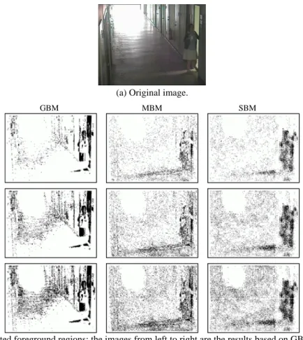
Fig. 6 (b) shows the results of a sample image captured by Cam2. The captured im-age is colored, and the colors of many parts of the person are similar to those of the background. The detected foreground regions of GBM and MBM are fragmental. Even though we apply a morphology-based hole filling procedure as shown in Fig. 6 (c), the foreground regions of the two methods are still fragmental. Thus, we can also conclude that SBM are more efficient than MBM and GBM.
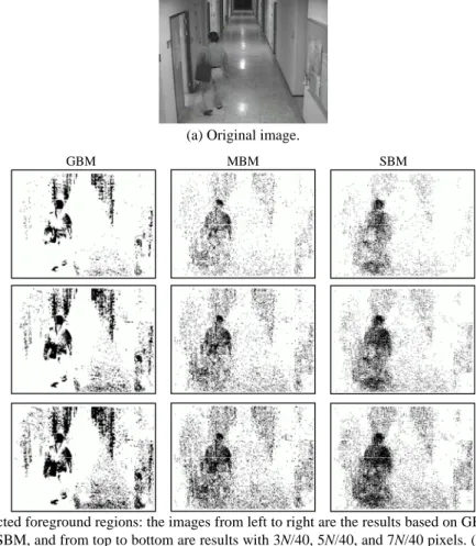
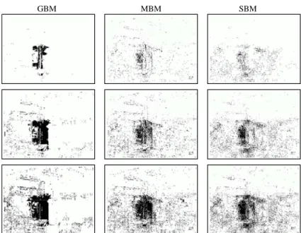
Fig. 7 (b) shows foreground detection results of a sample image captured by Cam3. Some of the regions of the door and its shadow are misclassified as foreground ones by using GBM and MBM, but not misclassified by using SBM. In the sample, since the door is opened when the person enters the room, the GBM does adapt to the current ap-pearance of the door and its shadow. In MBM, since the color distributions of the person,
(a) Original image.
GBM MBM SBM
(b) Detected foreground regions: the images from left to right are the results based on GBM, MBM, and SBM, and from top to bottom are results with 3N/40, 5N/40, and 7N/40 pixels. (N = image size).
(c) Foreground regions after noise removal.
Fig. 5. Foreground detection results of an image captured by Cam1.
door and shadow may all be modeled, the regions of these object may be misclassified. As shown in the middle column of Fig. 7 (b), the regions of the door and its shadow may also be misclassified or those of the person may be fragmental when an unsuitable seg-mentation threshold is set. By adopting SBM, the appearances of the person are not taken as background, since the joint colors of a pixel-pair in the person are not captured re-peatedly in the same position. The results in Fig. 7 (c) show that the person regions do not touch with background ones and less background regions are misclassified as fore-ground.
(a) Original image.
GBM MBM SBM
(b) Detected foreground regions: the images from left to right are the results based on GBM, MBM, and SBM, and from top to bottom are results with 3N/40, 5N/40, and 7N/40 pixels.
(c) Foreground regions after noise removal.
Fig. 6. Foreground detection results of an image captured by Cam2.
(a) Original image.
GBM MBM SBM
(b) Detected foreground regions: the images from left to right are the results based on GBM, MBM, and SBM, and from top to bottom are results with N/40, 3N/40, and 5N/40 pixels.
(c) Foreground regions after noise removal.
Fig. 7. (Cont’d) Foreground detection results of an image captured by Cam3.
Fig. 8 shows the foreground detection results of the images captured by the three cameras by setting a fixed threshold. The threshold that results in 15% false positive rate in training images is selected to test the performance of the models. The foreground re-gions depicted are noise removed. The results show that the foreground rere-gions extracted by SBM are more complete, and the false positive regions are less than those of the other two methods. The persons in Figs. 8 (a), (c) and (f) walk around a place. Since the ap-pearances of the persons are repeated in similar locations, the colors of the persons will be learnt as background by the pixel-wise background models GBM and MBM. In SBM, the colors of pixel-pairs will be modeled and the pixel-pairs without higher spatial de-pendency will be eliminated. Even though the appearances of a person are similar in a specific location, the joint colors of a pixel-pair in a fixed distance are usually varied and have low probabilities to be labeled erroneously as background. Note that the illumina-tions in these scenes are dramatically changed in Figs. 8 (e) and (f), when the lamplight is turned on, and slowly changed in Figs. 8 (a)-(d), when the illuminations are affected by the sunlight. In such environments, our proposed method is less affected by the illu-mination variations than others.
(a) (b) (c) (d) (e) (f) Fig. 8. Foreground detection results of the images captured by the three cameras. The images from
top to bottom are original images, the results of GBM, MBM, and SBM.
Cam1 Cam2 Cam3
Fig. 9. Test samples and the manually labeled ground truth masks used for estimating the ROC curves.
Figs. 10-12 show the receiver operating characteristic (ROC) curves of the video clips by controlling thresholds. The results of each figure are estimated from 20 randomly selected test images. These images all include moving persons. The ground truth data of the test samples are manually labeled as shown in Fig. 9. The results show that the curves of SBM and MBM are very similar and the true positive rates of SBM are usually higher than that of MBM. When we fix the true positive rate on 80%, the false positive rates are about 21% and 30% for the test images captured by Cam2 (Fig. 11) using SBM and MBM, respectively. The results show that we can eliminate about 30% (9% in 30%) misclassi-fied non-foreground pixels by extending MBM with spatial relations.
Note that the performances of GBM are usually better than those of MBM and SBM for the samples captured by Cam1 and Cam2 when the false positive rate is lower than 15%. The reason is that the background appearances do not change frequently in the cor-ridor. In the environment with less frequently changed background, a Gaussian distribu-tion can easily model the color distribudistribu-tion. However, when the background changes, the performance of GBM may become unacceptable for a fixed threshold as shown in Fig. 8.
Fig. 10. The ROC curve of test images captured by Cam1.
Fig. 11. The ROC curve of test images captured by Cam2.
Fig. 12. The ROC curve of test images captured by Cam3.
Although experimental results show that SBM usually outperforms MBM and GBM, the SBM is slower than the other two methods. The computation complex of calculating the background probability of a pixel of MBM is O(K), where K is the number of back-ground constituents, but SBM is O(K × M), where M is the number of pixel-pairs used. When we update the model of a pixel, the computation complex of MBM is still O(K), but SBM is O(K2 × M) since the computation cost of updating each weighting matrix is O(K2). On a PC with Pentium4 2 GHz CPU, the SBM can perform about one frame per- second, but the MBM is about 10 frames per-second. In our tests, about 90% CPU time spends on calculating the mutual information (Eq. (13)) and updating the matrix w (Eq. (10)).
6. CONCLUSIONS
In this paper, we have proposed a system to extract moving object regions from con-secutive images. Firstly, we have developed a spatial-extended background model for foreground detection. In the background model, we have used the probabilities of joint random vectors between near pixels to model the spatial relations. To reduce the cost of
modeling the pixel-pairs, we calculate the mutual information in each pixel-pair for find-ing the spatial-dependent pixel-pairs.
In general environments, when the background regions are stable, the Gaussian background model is suitable to segment foreground regions. However, when background regions change, the model is unsuitable. To detect foreground regions more accurately with respect to either changed or still background regions, we should combine our pro-pose model with Gaussian background model. To achieve this, some heuristic rules should be created for deciding which model should be selected. This is left for future studies.
REFERENCES
1. S. Shiry, Y. Nakata, T. Takamori, and M. Hattori, “Human detection and localiza-tion at indoor environment by home robot,” in Proceedings of IEEE Internalocaliza-tional Conference on Systems, Man, and Cybernetics, Vol. 2, 2000, pp. 1360-1365.
2. L. Wang, W. Hu, and T. Tan, “Recent developments in human motion analysis,” Pattern Recognition, Vol. 36, 2003, pp. 585-601.
3. A. Elgammal, R. Duraiswami, D. Harwood, and L. S. Davis, “Background and fore-ground modeling using nonparametric kernel density estimation for visual surveil-lance,” Proceedings of the IEEE, Vol. 90, 2002, pp. 1151-1163.
4. I. Haritaoglu, D. Harwood, and L. S. Davis, “W4: Real-time surveillance of people and their activities,” IEEE Transactions on Pattern Analysis and Machine Intelli-gence, Vol. 22, 2000, pp. 809-830.
5. C. Wren, A. Azarbayejani, T. Darrell, and A. P. Pentland, “Pfinder: Real-time track-ing of the human body,” IEEE Transactions on Pattern Analysis and Machine Intel-ligence, Vol. 19, 1997, pp. 780-785.
6. S. J. McKenna, S. Jabri, Z. Duric, A. Rosenfeld, and H. Wechsler, “Tracking groups of people,” Computer Vision and Image Understanding, Vol. 80, 2000, pp. 42-56. 7. A. Prati, I. Mikic, M. M. Trivedi, and R. Cucchiara, “Detecting moving shadows:
Algorithms and evaluation,” IEEE Transactions on Pattern Analysis and Machine Intelligence, Vol. 25, 2003, pp. 918-923.
8. R. Cucchiara, C. Grana, M. Piccardi, and A. Prati, “Detecting moving objects, ghosts, and shadows in video streams,” IEEE Transactions on Pattern Analysis and Ma-chine Intelligence, Vol. 25, 2003, pp. 1337-1342.
9. C. Stauffer and W. E. L. Grimson, “Learning patterns of activity using real-time tracking,” IEEE Transactions on Pattern Analysis and Machine Intelligence, Vol. 22, 2000, pp. 745-757.
10. D. S. Lee, “Effective Gaussian mixture learning for video background subtraction,” IEEE Transactions on Pattern Analysis and Machine Intelligence, Vol. 27, 2005, pp. 827-832.
11. H. Wang and D. Suter, “A re-evaluation of mixture-of-Gaussian background model-ing,” in Proceedings of IEEE International Conference on Acoustics, Speech, and Signal Processing, Vol. 2, 2005, pp. 1017-1020.
12. K. Kim, T. H. Chalidabhongse, D. Harwood, and L. Davis, “Real-time foreground- background segmentation using codebook model,” Real-Time Imaging, Vol. 11, 2005, pp. 172-185.
13. D. R. Magee, “Tracking multiple vehicles using foreground, background and motion models,” Image and Vision Computing, Vol. 22, 2004, pp. 143-155.
14. E. Durucan and T. Ebrahimi, “Change detection and background extraction by linear algebra,” Proceeding of the IEEE, Vol. 89, 2001, pp. 1368-1381.
15. L. Li, W. Huang, I. Y. Gu, and Q. Tian, “Statistical modeling of complex back-grounds for foreground object detection,” IEEE Transactions on Image Processing, Vol. 13, 2004, pp. 1459-1472.
16. L. Li and M. K. H. Leung, “Integrating intensity and texture differences for robust change detection,” IEEE Transactions on Image Processing, Vol. 11, 2002, pp. 105- 112.
17. Y. Wang, T. Tan, K. F. Loe, and J. K. Wu, “A probabilistic approach for foreground and shadow segmentation in monocular image sequences,” Pattern Recognition, Vol. 38, 2005, pp. 1937-1946.
18. R. O. Duda, P. E. Hart, and D. G. Stork, Pattern Classification, John Wiley and Sons, New York, 2001.
19. H. Deng and D. A. Clausi, “Unsupervised image segmentation using a simple MRF model with a new implementations scheme,” Pattern Recognition, Vol. 37, 2004, pp. 2323-2335.
20. C. K. Chow and C. N. Liu, “Approximating discrete probability distributions with dependence trees,” IEEE Transactions on Information Theory, Vol. 14, 1968, pp. 462-467.
21. S. L. Zhao and H. J. Lee, “Human silhouette extraction based on HMM,” in Pro-ceedings of the 18th International Conference on Pattern Recognition, Vol. 2, 2006 pp. 994-997.
San-Lung Zhao (趙善隆) received the B.S. and M.S.
de-grees in Computer Science and Information Engineering form National Chiao Tung University, Hsinchu, Taiwan, in 1998, and 2000, respectively. He is currently a Ph.D. student in Computer Science and Information Engineering, National Chiao Tung Uni-versity, Taiwan. His research interests include computer vision, image processing, and pattern recognition.
Hsi-Jian Lee (李錫堅) received the B.S., M.S., and Ph.D.
degrees in Computer Engineering from National Chiao Tung University, Hsinchu, Taiwan, in 1976, 1980, and 1984, respec-tively. From Aug. 1981 to July 2004, he had been with National Chiao Tung University as a Lecturer, Associate Professor and Professor. He was the Chairman of the Department of Computer Science and Information Engineering from Aug. 1991 to July 1997. From Jan. 1997 to July 1998, he was a Deputy Director of
Microelectronic and Information Research Center (MIRC). Since Aug. 1998, he had been the Chief Secretary to the president. Since Aug. 2004, he has been with Tzu Chi University, Hualien. From Aug. 2004 to Feb. 2006, he was the Chairman of the Depart-ment of Medical Informatics. From Apr. 2006, he has been the Dean of Academic Af-fairs. He was the editor-in-chief of the International Journal of Computer Processing of Oriental Languages (CPOL) and associate editor of the International Journal of Pattern Recognition and Artificial Intelligence and Pattern Analysis and Applications. His cur-rent research interests include document analysis, optical character recognition, image processing, pattern recognition, digital library, medical image analysis, and artificial in-telligence.
Dr. Lee was the president of the Chinese Language Computer Society (CLCS), Pro-gram Chair of the 1994 International Computer Symposium and the Fourth International Workshop on Frontiers in Handwriting Recognition (IWFHR) and was the General Chair of the Fourth Asia Conference of Computer Vision (ACCV), in January 2000.