Study of the acoustic feedback problem of active noise control
by using the l
1and l
2vector space optimization approaches
Mingsian R. Bai and Tianyau Wu
Department of Mechanical Engineering, Chiao-Tung University, 1001 Ta-Hsueh Road, Hsin-Chu, Taiwan, Republic of China
~Received 15 July 1996; revised 10 March 1997; accepted 8 April 1997!
This study attempts to explore the acoustic feedback problem that is frequently encountered in feedforward active noise control ~ANC! structure from the standpoint of control theories. The analysis is carried out on the basis of the Youla’s parametrization and the l1-norm and l2-norm
vector space optimization. The ANC problem is formulated as a model matching procedure and is solved via linear programming in the dual vector space. These methods alleviate the problems caused by the nonminimum phase~NMP! zeros of the cancellation path. The ANC algorithms are implemented by using a digital signal processor. Various types of noises were chosen for validating the developed algorithms. The proposed methods are also compared with the well-known filtered-u least-mean square ~FULMS! method. The experimental results show that the acoustic feedback problem significantly degrades the performance and stability of the ANC system regardless which method is used. Insights into the difficulties due to acoustic feedback are addressed along the line of control theories. © 1997 Acoustical Society of America.@S0001-4966~97!03008-7#
PACS numbers: 43.50.Ki@GAD#
INTRODUCTION
The active noise control~ANC! technique has attracted much academic as well as industrial attention since it pro-vides numerous advantages over traditional passive methods in attenuating low-frequency noises.1,2 However, the opti-mistic view somewhat masks the complexity of many theo-retical and technical problems that remain to be solved prior to full commercialization of the technique. Among the diffi-culties, the acoustic feedback problem of the feedforward structure has been the plaguing issue that seriously impedes successful application of the ANC technique. This problem usually arises in a feedforward ANC structure that is gener-ally the only practical approach for suppressing broadband random noises, where in many practical situations only the upstream acoustical reference is available. In this configura-tion, a positive feedback loop will exist between the cancel-ing loudspeaker and the feedforward microphone, which tends to destabilize the ANC system. Consider the ANC sys-tem for a duct shown in Fig. 1. Suppose that only the noise below the cutoff frequency of the duct is of interest so that the control problem can be treated as a one-dimensional problem. The secondary loudspeaker generates a canceling sound to interact destructively with the primary noise field. It is desired that the noise will be attenuated as much as pos-sible at the error microphone position. It is further assumed that only the acoustical reference at the upstream of the can-celing source is available, as usually is the case in practical applications. Unfortunately, the canceling loudspeaker on a duct wall will generate plane waves propagating both up-stream and downup-stream. Therefore, the antisound output to the loudspeaker not only cancels noise downstream by mini-mizing the error signals measured by the error microphone but also radiates upstream to the reference microphone, re-sulting in a corrupted reference signal. The coupling of the
acoustic wave from the canceling loudspeaker to the refer-ence microphone is called acoustic feedback.3Similar effects take place in the active vibration control system due to feed-back from the control actuator to the reference sensor. Be-cause the upstream feedforward microphone will detect both the noise from the primary source and the noise produced by the canceling loudspeaker, the positive acoustic feedback problem can no longer be ignored. It is this positive feedback problem that seriously complicates the active control design. The fact that acoustic feedback introduces poles to the system and thus a stability problem if the loop gain becomes too large has been illustrated by Eghtesadi and Leventhall.1,4 Another good review concerning acoustic feedback can be found in Chapter 3 of the book by Kuo and Morgan.3 The solutions to the problem of acoustic feedback cited in the book included directional microphones and loudspeakers, motional feedback loudspeakers, neutralization filter, dual-microphone reference sensing, the filter-u least-mean square
~FULMS! method, nonacoustic sensors, and so forth.
This paper adopts a new approach to explore the acous-tic feedback problem in the ANC application domain from the standpoint of control theories. The analysis is carried out on the basis of the Youla’s parametrization5 and the
l1-norm and l2-norm vector space optimization.6The perfor-mance of the developed methods is compared with the well-known FULMS algorithm that has long been recognized as one of the elegant solutions to the acoustic feedback problem.3,7 The simplicity of the proposed methods stems from the fact that the ANC problem is formulated as a model matching procedure and is solved via linear programming
~LP! in the dual vector space. These methods optimally
tackle the problem of unstable inverse resulting from the inherent nonminimum phase ~NMP! property of the cancel-lation path~which frequently occurs to structural systems or acoustical systems!.
The l1and l2ANC algorithms are implemented by using
a floating-point digital signal processor. Various types of noises including white noise, engine exhaust noise, and sweep sine were chosen for validating the developed algo-rithms. It will be seen from the experimental results that the acoustic feedback problem indeed significantly degrades the performance and stability of the ANC system regardless of which ANC method is used. Additional insights into the dif-ficulties due to acoustic feedback are also addressed in this paper within a general framework of control theories.
I. THEl1 ANDl2 ANC ALGORITHMS
The l1 control theory emerged in the 1980s. Dahleh and
Pearson proposed an l1 compensator to track persistent bounded signals.8The same authors also applied the l1 con-trol theory to reject bounded persistent disturbances by solv-ing a semi-infinite LP problem.9 Deodhare and Vidyasagar performed an in-depth analysis of the condition of when a stabilizing controller is l1 optimal.10 An excellent review of
the l1control theory can be found in the text by Dahleh and
Diaz-Bobillo.6 In the sequel, the l1 control theory is only
presented in the context of the ANC problem.
As mentioned previously, the acoustic feedback problem is very detrimental in terms of performance and stability of the ANC system. In what follows, the analysis of acoustic feedback problem in the ANC application domain is carried out from the standpoint of control theories. To begin with, the ANC problem is formulated as a model matching problem,11 as shown in the block diagram of Fig. 2. The sampled signal d(k) is the input disturbance noise and
y (k) is the residual field detected at the error microphone
position. The primary path, Pˆ (z), is the transfer function formed by the primary acoustic path, the power amplifier, the upstream sensor, and the error microphone, where z denotes the z transform variable. Sˆ(z) is the transfer function of the cancellation path formed by the canceling loudspeaker, the power amplifier, the secondary acoustic path, and the error microphone. Fˆ (z) is the transfer function of the acoustic feedback path formed by the canceling loudspeaker, the power amplifier, the acoustic path, and the upstream sensor. The transfer function Cˆ (z) represents the controller to be designed. In particular, Tˆ(z) is a transfer function describing the source dynamics formed by the primary source, a power
amplifier, an acoustical path, and the upstream microphone. Hence, the feedforward ANC problem in the presence of acoustical feedback amounts to finding the controller Cˆ (z) such that the residual field y (k) can be minimized. This is a generic model matching problem. That is,
min
C~z!
I
T~z!
F
P~z!1S~z! C~z!12F~z!C~z!
G
I
, ~1! where i~.!i is the notation of function norm. Note that the transfer function, Tˆ(z), can be regarded as a weighting func-tion for the terms inside the parenthesis. In practice, Tˆ(z) may not be measurable so that either analytical modeling or heuristic guess is needed.By Youla’s parametrization, the controller Cˆ (z) that guarantees the internal stability of the closed loop system can be expressed as12
Cˆ ~z!5Mˆ ~z!Qˆ~z!1Yˆ~z!
Nˆ ~z!Qˆ~z!1Xˆ~z!, ~2!
where Qˆ (z) is a stable, proper, and real-rational function
@denoted as Qˆ(z)PRH`#,12 Fˆ (z)5Nˆ(z)/Mˆ(z) is the
coprime factorization of Fˆ (z), and Xˆ(z)PRH` and Yˆ (z)
PRH` satisfy the Bezout identity12
Mˆ ~z!Xˆ~z!2Nˆ~z!Yˆ~z!51. ~3!
If the plant is proper and stable, as it is in our case, one may simply let12 Mˆ (z)51, Nˆ(z)5Fˆ(z), Xˆ(z)51, and Yˆ(z)50.
Then the controller in Eq. ~2! turns out to be
Cˆ ~z!5 Qˆ ~z!
Fˆ ~z!Qˆ~z!11. ~4!
Substituting Eq.~4! into Eq. ~1! leads to min
Q~z!PRH`
iT~z!@P~z!1S~z!Q~z!#i. ~5!
It is noteworthy that the model matching problem in Eq.~5! is exactly of the same form as that of the purely feedforward ANC system~in the absence of acoustic feedback! by replac-ing the designed controller Cˆ by a parameter Qˆ that is indi-cated by the dashed line in Fig. 2. Since Sˆ(z) is usually FIG. 1. Schematic diagram of the feedforward ANC structure for a duct in
the presence of acoustic feedback. FIG. 2. System block diagram of the feedforward ANC structure in the presence of acoustical feedback. Pˆ (z), Sˆ(z), Fˆ(z), and Cˆ(z) are the dis-crete time transfer functions of the primary path, the cancellation path, the acoustic feedback path, and the controller, respectively.
NMP, it is desirable to develop an algorithm that would ef-fectively match the primary path and the cancellation path with respect to some optimal criterion, especially when the NMP behavior is present. Elegant solutions to this problem are available in the robust control theory. Two model match-ing algorithms capable of dealmatch-ing with NMP problems in ANC applications are presented in this paper. The optimal solution of Eq. ~5!, Qˆopt(z), can be found by either l1 or l2
optimization procedure. min
QPl1
iP1S*Qi15 min HPl1
iG1Hi1
or ~6!
min
QPl2
iP1S*Qi25 min HPl2
iG1Hi2,
where P and S are pulse response sequences of the primary path and the cancellation path, respectively, ‘‘*’’ represents convolution, G5P, H5S*Q, ‘‘i•i1,2’’ denotes the 1-norm
or 2-norm, and l1 denotes the normed linear space of all
bounded sequences with bounded 1-norm.13
The following derivation contains a fair amount of mathematical definitions and results. However, the l1
theo-ries are quite standard in functional analysis14 and vector space optimization,13 and we present only the key ones needed in the development of the l1-ANC algorithm. The
rest are mentioned without proof.
The minimum distance problem in the primal space posed in Eqs.~6! can be recast into a maximum problem in its dual space. Let X be a normed linear space; f is said to be a bounded linear functional on X if f is a continuous linear operator from X to R. A dual space of X, denoted by X*, is the collection of all bounded linear functionals on X, equipped with the natural induced norm. Whenever f is rep-resented by some element x*PX*, we use the notation
^
x,x*&
to represent the value f (x). Then, a vector is said to be aligned with its normed dual if the following relation is satisfied13^
x,x*&
5ix*iixi. ~7! Given a sequence h5@h(1) h(2) h(3) •••#8
in l1, wherethe prime denotes matrix transpose, we also need the defini-tion ofl transform of h to facilitate the following derivations of l1 algorithm.
Hˆ ~l!5
(
k50`
h~k!lk. ~8!
Unlike the Z transform, it should be noted that the l trans-form is defined in terms of an infinite series of positive pow-ers. It is obvious that Hˆ (l) is BIBO ~bounded-input– bounded-output, i.e., both the input and the output are l` sequences! stable if and only if h is an l1 sequence.8 In
addition, the space c0 is defined as the space of all infinite
sequences in l` of real numbers converging to zero. With the aforementioned definitions, we are in a position to find the optimal solution of the model matching problem
in Eqs.~6!. Assume that Sˆ(l) has no zeros on the unit circle. Then the so-called interpolation constraints must be satisfied.8 Let Sˆ(l) have N NMP zeros denoted by ai, i
51,2,••• ,N, and uaiu,1, each of multiplicitygi, then Hˆ~k!~ai!50, i51,2,...,N; k50,1,...,gi21, ~9!
where the superscript (k) denotes the kth derivative of a complex function. The key of the solution to the optimiza-tion problem in Eqs. ~6! is based on the following duality
theorem.15
Theorem: Given the system of m consistent linear
equa-tions in n unknowns Ax5y, then min
Ax5y
ixip5 max
iA8uiq<1
~y
8
u!, ~10!where 1/ p11/q51, 1,p, q,`. Furthermore, optimal x and A
8
u are aligned. According to the theorem, the primalproblem~which is a minimization problem! can be converted to a maximization problem in its dual space. By the duality theorem, it can be shown that the l1 optimization problem in
Eq. ~6! becomes6
dopt5ifopti15 min V`8f5G
iG1Hi15 max
iV`xi`<1
~G
8
x!, ~11!where dopt is the minimal distance, f5G1H 5@a1 a2 a3•••#
8
is the error vector, foptis the optimalf,G5@Gˆ~a1!Gˆ~1!~a1!•••Gˆ~g1!~a1!Gˆ~a2!
3Gˆ~1!~a2!•••Gˆ~g2!~a2!•••Gˆ~gN!~a
N!#
8
, xPRm,and
V`5
F
Re~a10! ... Re~aN0! Im~a10! ... Im~aN0! Re~a11! ... Re~aN1! Im~a11! ... Im~aN1!
A A A A
G
.
In the matrix V`, Re.~•! and Im~•! denote the real part and the imaginary part, respectively. Note also that the interpo-lation constraints in Eq.~9! has been rewritten as V`
8
f5G. Hence the infinite-dimensional optimization problem has be-come a finite-dimensional one. The only pitfall is that the LP problem in Eq. ~11! has infinitely many constraints. How-ever, becauseuaiu,1, it can be shown that only a finitenum-ber of these constraints are really necessary.6More precisely, we can compute an integer, L, such that anyaisatisfies the
first L constraints also satisfies the remaining ones. Define a real Vandermonde matrix of order L
VL5
F
Re~a10! ... Re~aN0! Im~a10! ... Im~aN0! Re~a11! ... Re~aN1! Im~a11! ... Im~aN1!
A A A A
Re~a1L! ... Re~aNL! Im~a1L! ... Im~aNL!
G
.~12!
Hence, the matrix V`in Eq.~11! can everywhere be replaced by VL. If ai is real, then the column of zeros corresponding
to the imaginary part is dropped. If aiis complex, either aior
its complex conjugate a¯i is considered. Note that the matrix
the number of the constraints, L(>2N), can be computed a
priori:6
max
i
uaiuL~LuVL2lu1!,1, i51,2,...,N, ~13!
where VL2l is the left inverse of VL.
The beauty of the above l1 approach lies in the fact the
infinite-dimensional model matching problem in Eq.~11! has been converted to a standard LP problem described by
dopt5 max
iVLxi<1
~G
8
x!, ~14!which can be conveniently solved in the dual space by using an LP routine. Then the corresponding optimal solution is recovered in the primal space via the alignment conditions. Define
fL,opt5@a1 a2 ••• aL#
8
Pl1and
b5@b1 b2 ••• bL#
8
5VLxoptPC0.The l1 version of the alignment conditions are stated as:6,15 ~a!ai50 if ubiu,1; ~b!aibi>0 if ubiu51. However, only
part ~a! of the alignment conditions in conjunction with the interpolation constraints, VL
8
f5G, are needed for determin-ing the components offL,opt. AfterfL,opthas been solved,the finite-impulse response function fˆL,opt(z) can be ex-pressed~by using the fact l5z21! as
fˆ
L,opt~z!5a11a2z211•••1aLz2~L21!. ~15!
By the same token, the feedforward ANC problem can be formulated as an l2 model matching problem. The
mini-mization problem in the primal space can be converted to a maximization problem in the dual space by the duality theo-rem:
dopt5ifL,opti25 min
V L* 8 F5G iG2Hi25 max iVL*xi2<1 @G
8
x#, ~16! G5@Gˆ~a1!Gˆ~1!~a1!•••Gˆ~g1!~a1!Gˆ~a2!3Gˆ~1!~a2!•••Gˆ~g2!~a2!•••Gˆ~gN!~a N!#
8
,where the notations are the same as those defined in Eq.~11!. It can be shown that the alignment condition leads directly to the optimal solution5,14
fL,opt5VL~VL
8
VL!21G ~17!with the corresponding minimum distance
dopt5@G
8
~VL8
VL!21G#1/2. ~18!Note that the inverse of (VL
8
VL) is guaranteed since VL is offull column rank. The only difference between the l2
optimi-zation and the l1 optimization is that the former does not
require explicit solution of the dual problem.
Next, both the l1 and l2 optimal parameters, Qˆopt(z), can be obtained by backsubstituting fˆL,opt(z) into Eq. ~11!
or Eq.~16! as follows:
Qˆopt~z!5@fˆL,opt~z!2Pˆ~z!#/Sˆ~z!. ~19!
It should be noted that, because the interpolation constraints have been satisfied, the NMP zeros of Sˆ(z) will always be canceled by fˆL,opt(z)2Pˆ(z) to ensure the stability of the
parameter Qˆopt(z). After Qˆopt(z) is obtained, the optimal controller Cˆopt(z) can be recovered by the following
for-mula:
Cˆopt~z!5 Q ˆopt~z!
Fˆ ~z!Qˆopt~z!11. ~20!
A note regarding the implementation of the above l1
controller and l2 controller is in order. In some cases, it may
occur that these methods result in controllers with excessive gains in the high-frequency range. This is due to the fact that the control algorithms attempt to compensate for the NMP zeros in high frequencies that may be only artificially created from discretization.16 To alleviate the problem, remedies may be sought by incorporating a small constant e into
Sˆ(z), i.e.,
S~z!→@S~z!1e# ~21!
so that the plant is not excessively rolled off.
In some cases, the resulting controller Cˆopt(z) can be
unstable, even though the parameter Qˆopt(z) is guaranteed to
be proper and stable. This fact has been illustrated in an acoustic analysis in frequency domain of a simplified infinite-length duct model detailed in the paper by Eghtesadi and Leventhall.4An alternative argument from the viewpoint of control theory will lead to similar observation as follows. Let the transfer function between the disturbance d(k) and the residual output y (k) be Pˆ1(z). Recall that d(k) is
as-sumed to be inaccessible and only Pˆ (z)5Pˆ1(z)Tˆ21(z) is subject to some sort of experimental system identification procedure. However, it happens more often than never that the system, Tˆ(z), is NMP such that Tˆ(z) has no stable in-verse. Direct identification of the plant Pˆ (z) generally results in unstable or nearly unstable systems, even though both
Pˆ1(z) and Tˆ(z) are stable. Hence, it is likely that the
iden-tified Pˆ1(z) involves large modeling error and the best one
can get is only an approximation of the inherently unstable
Tˆ21(z). This approximation further degrades the perfor-mance of active control in comparison with the purely feed-forward structure. Nevertheless, this modeling difficulty can be alleviated somewhat by appropriate introduction of pas-sive damping. The importance of paspas-sive damping treatment that has often been overlooked in active design lies in not only high-frequency attenuation but also the robustness of active control with respect to plant uncertainties.17 Another benefit of using passive damping is that lower order of plant models can usually be obtained than the lightly damped plants so that numerical error is reduced.
II. EXPERIMENTAL RESULTS
Experiments were conducted to validate the adaptive l1
and l2ANC algorithms. A rectangular duct of length 1 m and
cross section 0.25 m30.25 m was chosen for this test. The duct is lined with fiberglass sound-absorbing material to create sufficient acoustical damping that is crucial to the
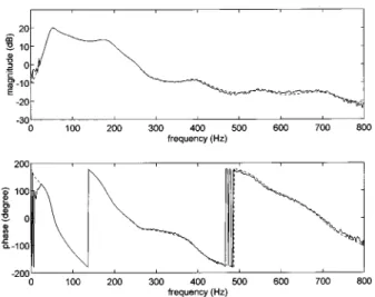
ro-bustness of the ANC system, as has been mentioned previ-ously. The corresponding cutoff frequency of the duct is 690 Hz and thus only plane waves are of interest. The controller was implemented by using a floating-point TMS320C31 digital signal processor. The sampling frequency was chosen to be 2 kHz. Fourth-order Butterworth filters with cutoff fre-quency 600 Hz were used as the anti-aliasing filter and the smoothing filter. The experimental setup including the duct, the upstream sensor, the error microphone, the actuator, the controller, and signal conditioning circuits has been shown in Fig. 1. The ARX system identification procedure18was used for establishing the mathematical models of the primary path, the cancellation path, and acoustic feedback path whose poles and zeros are listed in Table I. The frequency response functions of the primary path, the cancellation path, and the acoustic feedback path are shown in Figs. 3–5. The frequency response function of the chosen weighting func-tion in Eq. ~5! is shown in Fig. 6. The frequency response
FIG. 3. The frequency response function of the primary path Pˆ (z). Mea-sured data: ———; model data: ---.
TABLE I. The poles and zeros of the primary path Pˆ (z), the cancellation path Sˆ(z), and the acoustic feedback path Fˆ (z).
Pˆ (z) Sˆ(z) Fˆ (z)
Zeros Poles Zeros Poles Zeros Poles
9.9496 20.90286 0 0.96036 0 20.75216
21.7015 0.1998i 0 0.1314i 0 0.4749i
20.9043 20.9801 0 0.78226 0 20.81196
20.90676 20.8536 213.9155 0.4891i 2.04846 0.2015i
0.1871i 20.78816 1.0253 0.46606 1.8137i 20.47636
20.79566 0.3770i 0.9604 0.7756i 21.08376 0.7045i
0.3710i 20.71286 0.67636 0.58216 2.0421i 20.32626
20.71016 0.5819i 0.6445i 0.5469i 1.0389 0.7085i
0.5863i 20.59566 0.38386 0.11326 0.9233 20.09836
20.58526 0.6923i 0.7692i 0.8661i 0.63276 0.8864i
0.7100i 20.44396 0.13326 20.9756 0.6693i 0.32236
20.44146 0.7825i 0.8898i 20.24176 0.31436 0.8489i
0.7944i 20.39996 20.22286 0.8059i 0.7870i 0.22376
20.31016 0.7295i 0.7830i 20.73676 21.0706 0.7123i
0.8503i 20.29926 20.74196 0.3400i 20.84016 0.65906
20.15856 0.8666i 0.2637i 20.57246 0.3254i 0.6588i
0.9111i 20.14976 0.52606 0.5447i 20.05326 20.78006 0.06666 0.9207i 0.4643i 20.35826 0.7865i 0.4911i 0.9405i 0.07046 0.4790 0.6160i 20.49946 0.85016 0.27576 0.9221i 20.5067 0.6335 0.4428i 0.2237i
0.8730i 0.9975 20.23406 0.95796 0.50876 0.88806 0.6325i 0.1476i 0.8030i 0.2575i 20.7250 0.62326 0.88136 0.7250i 0.3695i 1.0075 0.79966 0.89026 0.4107i 0.2599i 0.75596 0.74636 0.5024i 0.5074i 0.80516 0.67926 0.4125i 0.6363i 0.56306 0.26536 0.1642i 0.8560i 0.50366 0.7872i 0.41526 0.6802i
functions of the optimal controllers designed by the afore-mentioned l1 and l2 procedure are then shown in Fig. 7.
To compare the performance of the ANC techniques, three types of noises including a white noise, a sweep sine, an engine exhaust noise were employed as the primary noises. The experimental cases and the associated noise types and control algorithms are summarized in Table II.
Case 1 is a reference case of purely feedforward l1
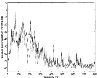
con-trol, where the source voltage signal is used as the feedfor-ward reference so that acoustic feedback can be neglected. It can be seen from the result of Fig. 8 that significant attenu-ation ~approximately 5–20 dB! is obtained in the frequency range 60–330 Hz. In cases 2–4, the signal detected by an upstream microphone is used as the feedforward reference so that the effect of acoustic feedback is present. In these cases, the widely used FULMS algorithm, the l1algorithm, and the l2 algorithm are employed for attenuating the white noise.
The power spectra of the residual fields at the error micro-phone position with and without active control are shown in Figs. 9, 10, and 11 for cases 2, 3, and 4, respectively. At-tenuation ~approximately 3–20 dB! was obtained from the FULMS method in the frequency range 50–200 Hz. The result was obtained 1 min after the active control was acti-vated. However, in Fig. 9, a strong peak was found at 235 Hz in the spectrum with the FULMS algorithm. On the other hand, attenuation ~approximately 2–30 dB! was obtained from the l1 and l2 method in the frequency range 50–220
Hz. Total attenuation within the dominant band 0–400 Hz is found to be 1.96 dB, 2.31 dB, and 2.93 dB for the FULMS method, the l1 method, and the l2 method, respectively.
Al-though the total attenuation appears to be comparable, these three control algorithms give different emphasis for different frequency ranges. The FULMS method produced most at-tenuation~approximately 20 dB! around 100 Hz, whereas the
l1and l2methods produced most attenuation~approximately
30 dB! around 200 Hz. The FULMS method is prone to have a stability problem, as compared with the l1method, and the
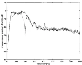
FIG. 4. The frequency response function of the cancellation path Sˆ(z). Measured data: ———; model data: ---.
FIG. 5. The frequency response function of the acoustic feedback path plant
Fˆ (z). Measured data: ———; model data: ---.
FIG. 6. The frequency response function of the chosen weighting function
Tˆ(z) in Eq.~5!.
FIG. 7. The frequency response functions of the l1and l2controllers in the
FIG. 8. The residual sound-pressure spectra of case 1 for the white noise in the absence of acoustic feedback before and after ANC is activated by using the purely feedforward l1controller. Control off: ———; control on: ---.
FIG. 9. The residual sound-pressure spectra of case 2 for the white noise in the presence of acoustic feedback before and after ANC is activated by using the FULMS and FXLMS controllers. The step sizes in FULMS and FXLMS are both 0.0001. The filter length in FULMS and FXLMS are 30 and 128, respectively. Control off: ———; FULMS: ---; FXLMS: –•–•.
FIG. 10. The residual sound-pressure spectra of case 3 for the white noise in the presence of acoustic feedback before and after ANC is activated by using the l1controller. Control off: ———; control on: ---.
FIG. 11. The residual sound-pressure spectra of case 4 for the white noise in the presence of acoustic feedback before and after ANC is activated by using the l2controller. Control off: ———; control on: ---.
TABLE II. Experimental case design.
Case Noise type Algorithm Tap/stepa Figure
1b white noise l
1 ••• 8
2 white noise FULMS 30/0.0001 9
3 white noise l1 ••• 10
4 white noise l2 ••• 11
5 sweep sine FULMS 30/0.0001 12
6 sweep sine l1 ••• 13
7 engine exhaust noise FULMS 30/0.0001 14
8 engine exhaust noise l1 ••• 15
a‘‘Tap/step’’ denotes the tap length and the step size used in the FULMS algorithm. b
control drifts away slowly so that the system may become unstable. This is probably because the performance index of the FULMS algorithm is not quadratic and the computation is easily trapped in local minima. In any rate, the detrimental effect of acoustic feedback is evidenced from these results. Regardless of which method is used, the performance of noise attenuation is significantly degraded in comparison with the purely feedforward control in case 1. For the sake of comparison, the filtered-x least-mean square ~FXLMS! method that is known to be effective for the purely ANC problems without acoustic feedback is also employed to tackle the same case. The result of Fig. 9 shows virtually no cancellation for the method. This is not totally unexpected since the optimal solution of the adaptive filter is generally an IIR function with poles and zeros when acoustic feedback is present.3 This rational function can only be approximated by an FIR function of infinitely long order. In practice, finite order of the FIR filter has to be used in conjunction with a very small step size for stability reasons. This results in
ex-tremely slow convergence in real applications. In the follow-ing cases, the results of FXLMS is thus omitted for brevity. In contrast to cases 2–4 that deal mainly with stationary noises, a sweeping sinusoidal noise is chosen in cases 5 and 6 to compare the effectiveness of the FULMS method and the l1 method in suppressing a nonstationary noise. The time-domain results of Figs. 12 and 13 show that the l1 method gives better performance than the FULMS method. This result is expected since the l1 controller is essentially a fixed controller that does not require adaptation time like the FULMS controller.
In cases 7 and 8, a practical noise, the engine exhaust noise, is employed as the primary noise for comparing the FULMS method and the l1method. The power spectra of the
residual fields at the error microphone position with and without active control are shown in Figs. 14 and 15. The result of the FULMS method was obtained 1 min after the active control was activated. Total attenuation within the dominant band 0–500 Hz is found to be 6.65 dB and 2.73 dB FIG. 12. The time-domain response of case 5 for the sweep sine in the
presence of acoustic feedback before and after ANC is activated by using the FULMS controller. The step size in FULMS is 0.0001. The filter length is 30. Control off: ———; control on: ---.
FIG. 13. The time-domain response of case 6 for the sweep sine in the presence of acoustic feedback before and after ANC is activated by using the l1controller. Control off: ———; control on: ---.
FIG. 14. The residual sound-pressure spectra of case 7 for the engine ex-haust noise in the presence of acoustic feedback before and after ANC is activated by using the FULMS controller. The step size in FULMS is 0.0001. The filter length is 30. Control off: ———; control on: ---.
FIG. 15. The residual sound-pressure spectra of case 8 for the engine ex-haust noise in the presence of acoustic feedback before and after ANC is activated by using the l1controller. Control off: ———; control on: ---.
for the FULMS method and the fixed l1 method,
respec-tively. Although cases 5–8 contain only the results of the FULMS method and the fixed l1 method, the l2 method
yields similar performance as the l1 method and the
corre-sponding results are omitted for brevity.
III. CONCLUSION
Acoustic feedback problem of the feedforward ANC structure is explored from the standpoint of control theories. Feedforward ANC systems based on l1and l2model
match-ing algorithms have been implemented by usmatch-ing a digital signal processor with acoustical feedback taken into account. The ANC algorithms are derived by using the Youla’s pa-rametrization and the l1-norm and l2-norm vector space
op-timization. These methods alleviate the problems caused by the nonminimum phase ~NMP! zeros of the cancellation path. Passive damping treatment was introduced to improve the robustness of the control design. It is found from the theoretical and experimental investigations that the acoustic feedback significantly complicates the control design and de-grades the performance and stability of the active control system because of the modeling error involved in approxi-mating the inverse source dynamics.
The performance of the l1 and l2 techniques was
com-pared experimentally with the well-known FULMS method in the presence of acoustic feedback for three kinds of noise. Although in some cases the total attenuation appears to be comparable, these active control algorithms provide different emphasis for different frequency ranges. The experimental investigations indicate the proposed methods have potential in suppressing not only stationary noises but also transient noises, where in the latter case the FULMS algorithm is gen-erally ineffective. This is not to mention the problem of sta-bility and local minima with the FULMS algorithm. That makes the proposed ANC systems attractive alternative for dealing with acoustic feedback problem in industrial appli-cations.
Despite the preliminary success, the performance of the ANC system is seriously limited by the undesirable acoustic feedback regardless of which method is used. In addition, the proposed controller is fixed in nature whose practicality will be limited in the face of system perturbations. Possibilities of different acoustic arrangements, different ANC structures
with more number of transducers that are unaffected by acoustic feedback, and an adaptive version of the l1/l2
con-troller will be explored in the future study.
ACKNOWLEDGMENTS
This paper was written in memory of late Professor Anna M. Pate, Iowa State University. Special thanks also go to Professor J. S. Hu for the helpful discussions on the l1
model matching principle. The work was supported by the National Science Council in Taiwan, Republic of China, un-der the Project No. NSC 83-0401-E-009-024.
1P. A. Nelson and S. J. Elliott, Active Control of Sound~Academic, New
York, 1992!.
2C. R. Fuller and A. H. von Flotow, ‘‘Active control of sound and
vibra-tion,’’ IEEE Control Systems Magazine, 9–19~December 1995!.
3S. M. Kuo and D. R. Morgan, Active Noise Control Systems: Algorithms and DSP Implementations~Wiley, New York, 1995!.
4
K. H. Eghtesadi and H. G. Leventhall, ‘‘Active attenuation of noise. The monopole system,’’ J. Acoust. Soc. Am. 71, 608–611~1982!.
5D. C. Youla, H. A. Jabr, and J. J. Bongiorno, Jr., ‘‘Modern Wiener–Hopf
design of optimal controllers, Part II: The multivariable case,’’ IEEE Trans. Autom. Control AC-21, 319–338~1976!.
6M. A. Dahleh and J. Diaz-Bobillo, Control of Uncertain Systems
~Prentice-Hall, Englewood Cliffs, NJ, 1995!.
7L. J. Eriksson, ‘‘Development of the filtered-u algorithm for active noise
control,’’ J. Acoust. Soc. Am. 89, 257–265~1990!.
8
M. A. Dahleh and J. B. Pearson, ‘‘l1-optimal feedback controllers for
MIMO discrete-time systems,’’ IEEE Trans. Autom. Control AC-32, 314–322~1987!.
9M. A. Dahleh and J. B. Pearson, ‘‘Optimal rejection of persistent
distur-bances, robust stability, and mixed sensitivity minimization,’’ IEEE Trans. Autom. Control 33, 722–731~1988!.
10G. Deodhare and M. Vidyasagar, ‘‘l
1-optimality of feedback control
sys-tems: The SISO discrete-time case,’’ IEEE Trans. Autom. Control 35, 1082–1085~1990!.
11
T. C. Tsao, ‘‘Optimal feedforward digital tracking controller design,’’ ASME J. Dynam. Syst. Measurement Control 116, 583–592~1994!.
12J. C. Doyle, B. A. Francis, and A. R. Tannenbaum, Feedback Control Theory~Maxwell Macmillan, New York, 1992!.
13
D. G. Luenberger, Optimization by Vector Space Methods~Wiley, New York, 1969!.
14W. Rudin, Functional Analysis~McGraw-Hill, New York, 1973!. 15J. A. Cadzow, ‘‘Functional analysis and the optimal control of linear
discrete systems,’’ Int. J. Control 17, 481–495~1973!.
16
K. J. Astrom, P. Hagander, and J. Sternby, ‘‘Zeros of sampled systems,’’ Automatica 20, 31–38~1984!.
17R. Gueler, A. H. von Flotow, and D. W. Vos, ‘‘Passive damping for
robust feedback control of flexible structure,’’ AIAA J. Guid. Control Dynam. 16, 662–667~1993!.
18
L. Ljung, System Identification: Theory for the User~Prentice-Hall, Engle-wood Cliffs, NJ, 1987!.