以奇異值調整法簡化模糊類神經網路

全文

(1)國立交通大學電機與控制工程學系碩士論文. 以奇異值調整法簡化模糊類神經網路 Simplification of Fuzzy Neural Network via Singular Value Regulation. 研究生：林育民指導教授：王啟旭. 教授. 中華民國九十四年十月.

(2) 以奇異值調整法簡化模糊類神經網路 Simplification of Fuzzy Neural Network via Singular Value Regulation. 研究生：林育民. Student：Yu-Min Lin. 指導教授：王啟旭. Advisor：Chi-Hsu Wang. 國立交通大學電機與控制工程學系碩士論文 A Thesis Submitted to Department of Electrical and Control Engineering College of Electrical Engineering and Information Science National Chiao Tung University in partial Fulfillment of the Requirements for the Degree of Master in Electrical and Control Engineering October 2005 Hsinchu, Taiwan, Republic of China. 中華民國九十四年十月. 2.

(3) 以奇異值調整法簡化模糊類神經網路. 學生：林育民. 指導教授：王啟旭. 國立交通大學電機與控制工程學系﹙研究所﹚碩士班. 摘. 要. 本論文提供一種縮減規則庫的方法來提升模糊類神經網路的效能。其核心理論為藉由調整由輸入輸出向量構成之模糊類神經網路矩陣的奇異值來改變輸入輸出之間的關係。我們稱此方法奇異值調整法。此方法可避免隨著輸出情況的高度複雜化而來之規則庫增加的問題。因此模糊類神經網路將有更好的效率。另外，因為模糊類神經網路是以小的規則庫來運作，其對應到規則庫的權重值可以很容易地以最小平方法得到。因此，模糊類神經網路對於輸出情況的變化將有更迅速的反應。我們藉由幾個例子來分析其誤差。所得到的結果證實由簡化過的規則庫仍可將精確度維持在很高的水平，因而大幅提升了模糊類神經網路的效率。. 3.

(4) Simplification of Fuzzy Neural Network via Singular Value Regulation Student：Yu-Min Lin. Advisors：Dr. Chi-Hsu Wang. Department of Electrical and Control Engineering National Chiao Tung University ABSTRACT The main purpose of this paper is to enhance the efficiency of a fuzzy neural network (FNN) by proposing a new training methodology with rule reduction. The core of this methodology is to modify the input-output relations by updating the singular value set associated with the FNN matrix, which is composed of the rule vectors and desired output vectors. We name it for Singular Value Regulation (SVR). By adopting this method, the FNN can have a better efficiency owing to it is free from extension of rule base, which often accompanies with high complexity of the situation described by the desired output. In addition, updating the weighting factor set associated with the rule base can be easily determined using least square method since the FNN often performs with a small size of rule base. Therefore, the FNN can have an instant response of the alternation of the output situation. Error analysis has been performed with illustrated examples. The outcome shows that the precision can be well maintained with the simplified rule base so that the efficiency of FNN is greatly enhanced.. 4.

(5) 致. 謝. 能完成這篇論文，首要感謝我的指導教授王啟旭在一年多當中給我的大力指導。使我能將雜亂的思緒理出頭緒。其次要感謝實驗室裡的同學和我分享他們的經驗，以及陳益生，蔡瑞昱學長給我學習上的幫助指點。另外要感謝的人是我的大學時代的導師朱一民教授對我的鼓勵以及給我寶貴的意見。也要感謝口試委員鄧清政，曾勝滄教授的指點批評。最後感謝我的父母對我的支持與犧牲奉獻，讓我能順利完成學業。. 5.

(6) Contents 摘要. …………………………………………………… 3. Abstract. …………………………………………………… 4. 致謝. …………………………………………………… 5. Chapter 1 Introduction……………………………………… 9 Chapter 2 Problem Formulation…………………………….. 11 Chapter 3 Singular Value Regulation (SVR)……………….. 15 3.1 Singular Value Decomposition (SVD)……………... 15 3.2 Singular Value Regulation (SVR)………………….. 16 3.3 Improved training strategy…………………………. 21. Chapter 4 Reduction of Rule Base………………………….. 29 Chapter 5 Illustrative Examples………………………….…. 32 Conclusion …………………………………………………………… 45 Reference …………………………………………………………… 46. 6.

(7) List of Figures Figure 1 Configuration of Fuzzy neural network……………….……………. 3 Figure 2 Vector space distribution in the case with large error...….….. 4 Figure 3 Vector space distribution in the case with small error……….. 5 Figure 4 Vector space distribution in the ideal case……………………... 5 Figure 5 Rule base transformed by regulating singular value.…….……..…. 10 Figure 6(a) Feasible paths for navigation……………………….…………...…... 16 Figure 6(b) Output training pattern for the navigated object……………… 17 Figure 6(c) Membership functions for controlling the turning angle and speed 17 Figure 6(d) Configuration of fuzzy neural network in two different cases.. .17 Figure 7(a) Outcome of the generated paths in case1……………………….. 19 Figure 7(b) Outcome of the generated paths in case1…………………….……... 19 Figure 8 A feasible path for car navigation…………………………………... 24 Figure 9 Membership functions defined for generating the feasible Paths………………………………………………………………….. 25. Figure 10 Paths generated by twenty-seven rules…………………….……. 27 Figure 11 Paths generated by reduced rule base…..………………………. 29 Figure 12 Two general cases for car navigation………….………………… 30 Figure 13 (a) Paths generated from the reduced rule base without tuning… 30 Figure 13 (b) Paths generated from the reduced rule base tuned by removing Singular value………….…….………………………………………. 31. 7.

(8) Figure 14 Comparison of navigated paths generated from tuned rule base and the original rule base….………………………………………… 31. Figure 15 Advantage of tuning rule base………………….…………………… 33 Figure 16 System identified by reduced rule base……………..………………. 36 Figure 17 Step response of the identified system…………………………… 36. List of Tables Table 1. Weighting factor set obtained from different algorithms………... 26. Table 2. Comparison of errors obtained from different algorithms……… 28. Table 3. Singular Values of the FNN matrix associated with the car navigation problem…………………………………………………. 33. Table 4. Rule base set for car navigation problem. 34. Table 5. The corresponding weighting factors associated with rules for car navigation……………………………………………………….. Table 6. 35. Correlations between rules and desired outputs associated with the special case……………………………………………………… 40. Table 7. Fuzzy sets associated with system identification of the plant model………………………………………………………………… 42. Table 8. The corresponding weighting factors associated with rules for system identification problem…………………………………..….. 8. 42.

(9) Chapter 1 Introduction Controlling the relationship between inputs and outputs is an important issue for many engineering problems, for the reason that it is usually required that some desired output be presented by a given set of input variables. However the system model may not be well understood. Thus they may have to be approximated by a given set of input-output training data. The given training data may result from experiments, real world conditions,…, etc. In recent years, the FNN (Fuzzy Neural Network) [1] has been developed to generate the desired outputs with given fuzzy inputs. The major work for building the FNN is defining the fuzzy rule base. The rule base is also called knowledge base, which is derived from human feeling. Theoretically, to have a large set of training data is essential for dealing with all the possible situations precisely. However, it will cause a vast rule base. Apparently, the generating efficiency will be much decreased using such a vast rule base due to high redundancy of rules frequently exists when dealing certain simple cases. Therefore, the reduction of rule base becomes a critical issue. Some related works has been done in previous papers. In [2], two strategies are proposed in dealing with the foundation of fuzzy rules: 1) rule generation by refinement, 2) rule reduction by merging. The former discusses the necessity of each rule, and the latter discusses rule expansion technique that enlarges the valid boundaries of rules and in turn reduces the rule base. A novel approach in [3] is also proposed to perform vector selection based on the analysis of class regions, which are generated by a fuzzy classifier. The exception ratio is a vital concept in [3] to determine the necessity of rules. The definition of exception ratio is the degree of overlaps in the class regions. The idea of using the exception ratio for feature evaluation derives from the fact that given a set of features, a subset of features that has the lowest sum of the exception ratios has the tendency to contain the most relevant features, compared to the other subsets with the same number of features [3]. The approach to minimize the rule base is to reduce the exception ratio. Another popular method for reducing the redundancy of rules is performing singular value decomposition (SVD), which has been discussed in [4, 5]. However, it may be time consuming suppose the redundancy of rules is high 9.

(10) since redundant rules are taken into account during the training process instead of being eliminated initially.. Though reduction of rule base improves the efficiency of FNN, it also reduces the certain conditions given from human beings so that the FNN becomes more constrained in dealing with some specific cases. In other words, it is difficult to well concern all the possible situations concurrently with keeping high precision. Furthermore, we may not sure whether the specific rules are valid to be removed or not owing to insufficiency of knowledge and uncertainty of information. Thus we propose an advance approach to well tune the rule base such that the FNN can deal with multiple situations with a simpler rule base. The idea of this approach is derived from the concept of singular value decomposition (SVD), and thus the analysis of singular values via performing SVD is vital for analyzing its performance. Some examples are fully illustrated to yield satisfying results such as the model car navigation and nonlinear system identification problems in [1, 7]. The outcome shows that by adopting this approach, the precision can be well maintained with much simpler rule base so that the efficiency is much improved.. 10.

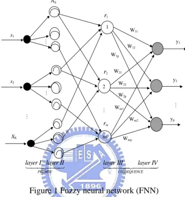
(11) Chapter 2 Problem Formulation The topic of this paper is relevant to improving the efficiency of Fuzzy Neural Network (FNN), which has the configuration shown in Figure 1[1]. Aij. r1 1. W11. x1. y1. W12 W1p. r2 W21 x2 2. y2. W22 W2p Wm1 Wm2. rm XK. m. layer I layer II. Wmp. layer III. PREMISE. yp. layer IV. CONSEQUENCE. Figure 1 Fuzzy neural network (FNN). There are four layers in this structure. The input variable is fed into the first layer, then operated by the mappings A1(x1), A2(x2)…. Ak(xk) in the second layer. The nodes of third layer are corresponding to different rules, which are derived from multiplying the products fuzzy mapping associated with each rule. Thus the value of rule at a certain sampling instant is derived from the following equation: k. r (t ). = ∏ Ai ( x i ( t )). (1). i =1. Where Ai(xi(t)) represents the fuzzy mapping associated with the ith input variable, and t denotes the sampling instant. The third layer is also called hidden layer. The fourth layer is the output variables. The transition from layer three to layer four is via the simple two layer neural network with the weighting factor to be decided. The output variable is utilized to approximate the desired output. The way we attempt to find out the output of FNN is to find out the appropriate. 11.

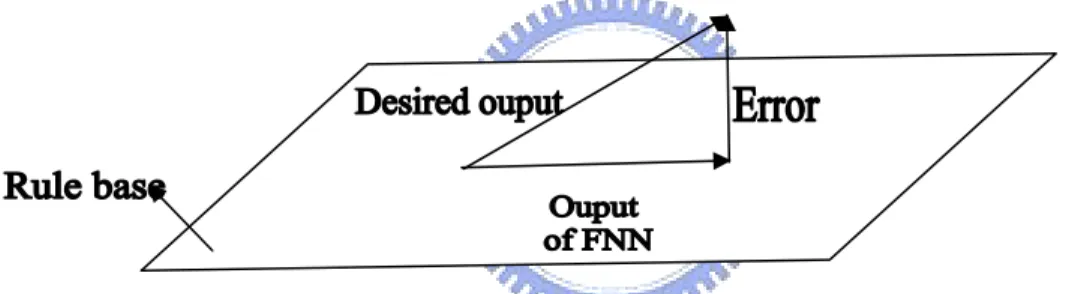
(12) weighting factor associated with each rule followed by combining them as the following form: f (t ) = w1r1 (t ) + w2 r2 (t ) + w3 r3 (t ) +. + wm rm (t ). (2). Where f(t) is the generated output of FNN, and ri(t) represents the ith rule. Apparently, the output is supposed to be linearly dependent on the given rule set under the convention shown in (2). However, this is usually not the real case. This means the linear relation between rules and desired output is usually an approximation of the real situation. Thus, the desired output d(t) should be expressed as: d (t ) = w1r1 (t ) + w2 r2 (t ) + w3r3 (t ) +. + wm rm (t ) + e(t ). (3). Compare (2) and (3), the desired output belongs to the vector space whose rank is higher than that of the vector space spanned by rule base. The phenomenon is illustrated in the following figure:. Figure 2 Relationship of rule base, desired output, error and output of FNN.. The error is minimized as the generated output is the orthogonal projection of desired output, which is composed of products of the rule base and the optimal weighting factor set that obtained from least square method [8], which can be described as the following equation:. (. w = RRT. ). −1. Rvd. (4). Where vd = [d(t1), d(t2), d(t3),……., d(tn)]T ⎡ r1 (t1 ) r1 (t2 ) r1 (t3 ) r1 (t4 ) ...... ⎢ r (t ) r (t ) r (t ) r (t ) ...... 2 2 2 3 2 4 ⎢ 2 1 R = ⎢ r3 (t1 ) r3 (t2 ) r3 (t3 ) r3 (t4 ) ...... ⎢ ⎢ ⎢⎣ rm (t1 ) rm (t2 ) rm (t3 ) rm (t4 ) ....... 12. r1 (tn ) ⎤ r2 (tn ) ⎥⎥ r3 (tn ) ⎥ ⎥ ⎥ rm (tn ) ⎥⎦ m × n. (5). (6).

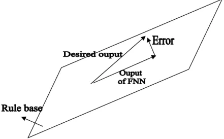
(13) Obviously, the least square error decreases suppose that the rule base is getting closer to the vector space where the desired output belongs, which can be shown in the following figure:. Figure 3 Case with smaller error. The vector space where the desired output belongs is closer to that spanned by rule base compared with the case in figure 2.. From the above illustration, the error decreases with reducing the inconsistence of vector spaces. This implies that the error disappears provided that the desired output and the rule vectors are merged into the same vector space, such as shown in the following figure:. Figure 4: The relationship between desired output and rule base in the ideal cases.. Thus, the key issue to be concerned is rank of vector space where the following vectors belong:. 13.

(14) v1. =. ⎡⎣ r1 ( t 1. v2. =. ⎡⎣ r 2. ). (t1 ). r1 ( t 2 r2. ). r1 ( t n ) ⎤⎦. (t 2 ). r2. T. ( t n ) ⎤⎦. T. (7) vm. =. ⎡⎣ r m. v dj. =. ⎡⎣ d. j. (t1 ). rm. (t1 ). d. (t 2 ) j. (t 2 ). rm. d. ( t n ) ⎤⎦ j. T. ( t n ) ⎤⎦. T. Where r1~rm are rule vectors, and vdj represents the jth desired output number. P and m represent the number of rules and number of desired outputs respectively. n is assumed to be far larger than p+m, i.e., n>>p+m. It is known that the rank can be found by inspecting the singular values of matrix comprising the vectors to be analyzed. Consequently, we set a matrix built from the vectors in (7), such as: ⎡ d1 (t1 ) ⎢ ⎢ d1 (t2 ) G = ⎢ d1 (t3 ) ⎢ ⎢ ⎢ d1 (tn ) ⎣. d p (t1 ) r1 (t1 ) d p (t2 ) r1 (t2 ) d p (t3 ) r1 (t3 ) d p (tn ) r1 (tn ). rm (t1 ) ⎤ ⎥ rm (t2 )⎥ rm (t3 )⎥ ⎥ ⎥ rm (tn )⎥⎦ n × ( p + m). (8). We name the matrix in (8) FNN matrix owing to it is adopted frequently in this paper. The redundancy of singular values of FNN matrix demonstrates the linearity between rule vectors and desired output vectors. Ideally, vdj (j =1~p) are exactly linearly dependent on v1~vm, which implies p redundant vectors exist in the FNN matrix so that it contains p zero singular values. However in real situation, trivial singular values instead of zero singular values are found. This implies the linearity is changed with replacing these trivial singular values by zeros, which is the main idea of the proposed approach in this paper. The approach will be discussed in detail in the following chapter.. 14.

(15) Chapter 3 Singular Value Regulation (SVR) Singular Value Decomposition (SVD) will be discussed first in this chapter. Then Singular Value Regulation (SVR) based on SVD, will be addressed next. A tuning algorithm based on singular value regulation (SVR) will also be proposed in this chapter.. 3.1 Singular Value Decomposition (SVD) The core of tuning approach proposed in this paper is relevant to singular values. Consequently, Singular Value Decomposition (SVD) is an essential approach to be analyzed first. The fundamental of singular value decomposition (SVD) is to express the analyzed vector set in terms of the eigenvectors belonging to the matrix consists of all the vectors in the analyzed vector set [9~14]. Here, the vectors to be analyzed are rule vectors and desired output vectors. Suppose we have p desired outputs (x1~xp) and m rules (xp+1, xp+2, …, xp+m), combined together in an FNN matrix G such as. ⎡ G = ⎢ x1 ⎣. x2. x p x p +1. ⎤ x p+m ⎥ ⎦ n×( p + m ). (9). Because the new basis is composed of the eigenvectors of G, we have to find the left eigenvectors ui (1 × n row vector) and right eigenvectors vi ((p+m) × 1) column vector such as: G T Gvi = σ i 2 vi ui GG T = ui σ i 2 vi. = ⎡⎣ vi1 vi 2. vi ( p + m ) ⎦⎤. ui. =. [ui1. uin ]1×n. ui 2. T. (10). 1×( p + m ). Where σi. (i=1~p+m) are the singular values of G. Actually, the validity of finding the left and right eigenvectors of FNN matrix G via the equations shown in (10) implies the existence of following equation: G=U∑VT. (11). Where U and V are composed of ui (i =1~n) and vi (i =1~p+m) respectively. ∑ is the diagonal 15.

(16) matrix composed of singular values of FNN matrix G. We focus our concern on vi because it is associated with the column vectors of G which are going to be analyzed. The component of all the data set on the eigenvector vi can be shown as:. = vi1 x1 + vi 2 x2 +. xi*. + vi ( p + m ) x p + m. (12). or xi*. = Gvi. (13). Where “*” denotes transformed vector set derived form expressing the original vectors in terms of new basis (i.e., the set of eigenvectors of G). It is obvious that GTG is a symmetric matrix so that its normalized eigenvectors (i.e., vi) forms an orthonormal set. Consequently, we can have the following (14) from (10) and (13): xi*T xi*. = viT G T Gvi = σ i2 viT vi = σ i2 = || xi* ||2. (14). From (14), the importance of singular value can be analyzed from its associated transformed vector. This fact will be adopted extensively in the following sections.. 3.2. Singular Value Regulation. As previously mentioned, the maximum rank of FNN matrix G in (8) is m, provided that rule base and desired output are in the same vector space. However, this is not true in real situations. We can only assume that rule base and desired outputs are approximately in the same vector space in real situations. Therefore, we cannot fully neglect the contribution of insignificant singular values of FNN matrix G because they do not exactly equal to zeros. The key technique for singular value regulation (SVR) algorithm is to force insignificant singular values of FNN matrix G defined in (8) to zeros such that desired outputs are in the vector space spanned by rule base. Therefore desired outputs can be exactly expressed as a sum of products of weighting factors and their associated rules, such as shown in (2). The overall procedure for regulating singular values is induced as the following algorithm:. Algorithm1: Tuning FNN via Singular Value Regulation (SVR) 16.

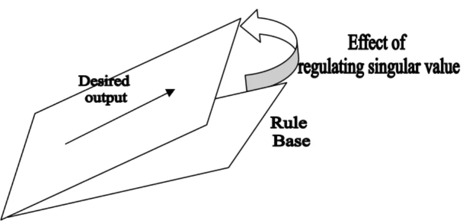
(17) The FNN shown in Figure 1 has k input fuzzy variables, {x1(t), x2(t),…, xk(t)}, and p desired outputs {d1(t), d2(t) , …, dp(t)} with m fuzzy rules {r1(t), r2(t), …, rm(t)}. Given: Input training data: {x1(ti), x2(ti ),…, xk(ti )}. Desired outputs: {d1(ti), d2(ti) , …, dp(ti)}. Rule base: {r1(ti), r2(ti) , …, rm(ti)}. Where ti denotes the ith sampling instant (i=1~n). Goal: Tune the FNN so that the actual outputs can be as close as possible to the desired outputs.. Step 1: Construct a matrix denoted G whose column vectors consist of sample values of rules and desired outputs, which is the FNN matrix. Step 2: Perform singular values decomposition on G. That is to transform G as the following form: G = U ΣV T Where U, Σ, V are defined in (11). Step 3: Create another matrix Σ’ from Σ by replacing the p least significant singular values of Σ with zeros and keeping the rest m singular values of Σ untouched. Step 4: Create another FNN matrix G’ by using U, Σ’, VT (derived from Step2 and Step3) such as: G ' = U Σ 'V T The column vectors in FNN matrix G’ are the tuning result, which consists of tuned rule vectors and desired output vectors. Step 5: Find the weighting factors associated with the tuned rule vectors obtained in Step 4 by Eq. (6), which is based on least square method. Step 6: Find the desired outputs by summing the products of rules and their associated weighting factors.. The core of the above algorithm is regulating singular values, which has the impact on the vector space shown in following figure:. 17.

(18) Figure 5: Rule base transformed by regulating singular values.. Figure 5 shows that the rule base is tuned by regulating singular values. The effect can be expressed as adding a deviation on each sample value of rules. That is:. r1 (ti ) → r1 (ti ) + ∆r1 (ti ), r2 (ti ) → r2 (ti ) + ∆r2 (ti ),. rm (ti ) → rm (ti ) + ∆rm (ti ). d1 (ti ) → d1 (ti ) + ∆r1 (ti ), d2 (ti ) → d2 (ti ) + ∆d2 (ti ),. d p (ti ) → d p (ti ) + ∆d p (ti ). ( i = 1 ~ n) ( i = 1 ~ n). Where n, m, p denote the number sampling instants, rules, and desired outputs respectively. The deviations (i.e., ∆r1 (ti ), ∆r2 (ti ), base (i.e., r1 (ti ), r2 (ti ),. ∆rm (ti ) ) are utilized to modify the originally defined rule. rm (ti ) ) while the FNN is dealing with some special situations that. cannot be well performed via the original rule base. The tuning approach makes the rule base and desired outputs merge into the same vector space so that the desired outputs are exactly linear combinations of rules. That is, the desired outputs are exact the combinations of rules and the optimal weighting factor set obtained from Least Square Method. Thus, the error between actual output of FNN and desired output exactly depends on the deviations resulting from regulating singular values, which are:. ∆d1 (ti ), ∆d2 (ti ),. ∆d p (ti ). (i = 1~ n). To be specific, suppose we wish to approximate the desired outputs (i.e., x1, x2,…, xp) via the linear combination of rule vectors, (i.e, xp+1, xp+2,…, xp+m) as precisely as possible. That is, we expect the error defined in the following equation to be small.. 18.

(19) (15) Where wi are the weighting factors to be determined and e is the error. Since the error is not zero, x1 is “approximately” linearly dependent on rule base (i.e, xp+1, xp+2,…, xp+m). After performing SVD on FNN matrix G and removing the p least significant transformed vectors xi*, we have the new vector set which is deviated from the original ones, such as: xi' = xi +∆xi ; i = 1, 2,..., p + m.. Where xi’ represents the vector obtained by removing the projection of xi on xi* (i = m+1~m+p) defined in previous section. ∆xi (i = 1~p+m) are the deviations between original vectors and tuned vectors. However the removal of these xi* reduces the rank of FNN matrix G by p. This implies that any column vector in G can be an “exact” linear combination of the other column vectors. Then we can have: m. x j = ∑ wi* xi'. ( j = 1 ~ p, i = p + 1 ~ p + m). (16). i =2. The above (16) represents the relationships between rules and desired output of FNN; wi*(i= p+1~p+m) are weighting factors to be determined. From (15) and (16), it is obvious that the error is exact equal to the deviation between xi’ and xi resulting from removal of singular values. σi (i =m+1~m+p). We can analyze the deviation by defining the norm of FNN matrix G defined in (9) via the result derived from (14), i.e., ⎛ p+m * ⎞ G =⎜ xi ⎟ ⎜ ⎟ i 1 = ⎝ ⎠. ∑. 1. 2. ⎛ p+m 2 ⎞ σi ⎟ =⎜ ⎜ ⎟ i 1 = ⎝ ⎠. ∑. 1. 2. (17). From (14) and (17), the percentage error for FNN matrix G resulting from removal of certain singular value can be described as follows: Percentage error (i) =. σ i2. =. p+m. ∑σ k =1. 2 k. || xi* ||2. (18). p+m. ∑ || x k =1. * k. ||. 2. Actually, the removed part of the specific vector xj is only part of ||xi*||. To be more specific, we examine the error associated with specific vector xj (i.e., ∆x j ( m +1) ) from the following equations:. 19.

(20) x. j. ⎡ m ⎢ ∑ σ q u1q v qj + σ ⎢ q =1 ⎢ m ⎢ ∑ σ q u 2 q v qj + σ = ⎢ q =1 ⎢ ⎢ m ⎢ ⎢ ∑ σ q u nq v qj + σ ⎣ q =1. ⎤ u 1( m +1) v ( m +1) j ⎥ ⎥ ⎥ m +1u 2 ( m +1) v ( m +1) j ⎥ = x 'j + ∆ x ⎥ ⎥ ⎥ ⎥ m +1u n ( m +1) v ( m +1) j ⎥ ⎦ n ×1 m +1. j ( m +1). (19). Where. ∆x. j ( m +1). ⎡ σ m +1u 1( m +1) v ( m +1) j ⎢σ m +1u 2 ( m +1) v ( m +1) j = ⎢ ⎢ ⎢ ⎣⎢ σ m + 1 u n ( m + 1 ) v ( m + 1 ) j. ⎤ ⎥ ⎥ , ⎥ ⎥ ⎦⎥ n × 1. x 'j. ⎡ m ⎢ ∑ σ q u1q v qj ⎢ q =1 ⎢ m ⎢ ∑ σ q u 2 q v qj = ⎢ q =1 ⎢ ⎢ m ⎢ ⎢ ∑ σ q u nq v qj ⎣ q =1. ⎤ ⎥ ⎥ ⎥ ⎥ ⎥ ⎥ ⎥ ⎥ ⎥ ⎦ n ×1. (20). Thus we have:. ∆ x 2j ( m +1) = σ i2 vi2( m +1). (21). Compare (14) and (21), the deviation of xi is reduced by a coefficient vij2 compared with the removed singular values σi2. This confirms that the error associated with desired output can be kept small in performing singular value regulation. However, for multiple desired outputs case, the removed singular values tends to have more effect on precision since the error caused by removing singular values should be updated as: m+ p. ∑. i = m +1. σ i2 v i2 , or. m+ p. ∑ || x. i = m +1. * i. ||2 vi2. (23). Apparently, the number of desired output should be reduced for high precision requirement. However, it may be conflict with real situations. Thus we propose an improved training strategy, which will be discussed in the following section.. 20.

(21) 3.3. Improved Training Strategy. The above (23) demonstrates that the error grows up with increasing the quantity of desired outputs. Thus, the extension of rule base may be essential for maintaining high precision. To be specific, consider the following two training cases: Case 1: Generating the desired outputs via tuning a large size of rule base. σ , σ , , σ , σ , σ uiσ ui , , σ ui m sin gularvalues. p sin gular values. Case 2: Generating the desired outputs via tuning a small size of rule base. σ , σ , σ , σ , σ , , σ ui , σ ui m sin gularvalues. p sin gular values. Where m and p are number of rules and number of desired outputs respectively. σui represent the unimportant singular values. In case 1, the least p significant singular values are safe to be eliminated since m >> p. While the error in case 2 is considerable due to some of important singular values may be treated as zeros. However, for high efficiency requirement, case 2 is the better choice due to the rule base to be considered is smaller. Thus our objective is to reduce the number of desired outputs to be generated. This can be accomplished by replacing the convention of FNN matrix as the following form: ⎡ d1 (t11 ) r1 (t11 ) ⎢ ⎢ ⎢ d1 (t1n ) r1 (t1n ) ⎢ ⎢ d 2 (t21 ) r1 (t21 ) ⎢ G= ⎢ ⎢ d 2 (t2 n ) r1 (t2 n ) ⎢ ⎢ ⎢ d p (t p1 ) r1 (t p1 ) ⎢ ⎢ ⎢ d p (t pn ) r1 (t pn ) ⎣. rm (t11 )⎤ ⎥ ⎥ rm (t1n )⎥ ⎥ rm (t21 )⎥ ⎥ ⎥ rm (t2 n )⎥ ⎥ ⎥ rm (t p1 )⎥ ⎥ ⎥ rm (t pn )⎥⎦ pn × (m + 1). By utilizing the convention of FNN matrix shown above, the error is much reduced since it is simply determined from the weight of the least significant singular value. Based on this 21.

(22) advantage, the desired output can be generated from a much simpler rule base so that the quantity of training data and weighting factors to be deal with can be much reduced. Furthermore, the extraction of dominant rule base does not have to be performed since the rule base has been kept small. Thus the efficiency of FNN is indeed improved.. By adopting the improved training strategy, Algorithm1 should be modified, as shown in the following Algorithm 2.. Algorithm2: Tuning FNN via SVR algorithm with improved training strategy The FNN shown in Figure 1 has m fuzzy rules {r1(t), r2(t), …, rm(t).with p desired outputs {d1(t), d2(t) , …, dp(t)}. Given: Desired outputs: { d1(tji), d2(tji), d3(tji),..., dp(tji) } Rule base: {r1(tji), r2(tji ) , …, rm(tji )}. Where tji denotes the ith (i=1~n) sampling instant associated with jth desired output. Goal: Tune the FNN so that the actual outputs can be as close as possible to the desired outputs.. Step 1: Construct the associated FNN matrix G, which is: ⎡ d1 (t11 ) r1 (t11 ) ⎢ ⎢ ⎢ d1 (t1n ) r1 (t1n ) ⎢ ⎢ d 2 (t21 ) r1 (t21 ) ⎢ G= ⎢ ⎢ d 2 (t2 n ) r1 (t2 n ) ⎢ ⎢ ⎢ d p (t p1 ) r1 (t p1 ) ⎢ ⎢ ⎢ d p (t pn ) r1 (t pn ) ⎣. rm (t11 )⎤ ⎥ ⎥ rm (t1n )⎥ ⎥ rm (t21 )⎥ ⎥ ⎥ rm (t2 n )⎥ ⎥ ⎥ rm (t p1 )⎥ ⎥ ⎥ rm (t pn )⎥⎦. pn × (m + 1). Step 2:Perform singular value decomposition on G. This is to transform G into the following form: G = U ΣV T 22.

(23) Where U, Σ, V are defined in (11). Step 3:Create another matrix Σ’ from Σ by replacing the least significant singular value of Σ with zero and keeping the rest singular values of Σ untouched. Step 4: Reconstruct G’ by using U, Σ’, VT (derived from Step 2 and Step 3) such as: G ' = U Σ 'V T The column vectors in FNN matrix G’ are the tuning result, which consists of tuned rule vectors and the desired output vector. Step 5: Find the weighting factors associated with the tuned rule vectors obtained in Step 4 by least mean square (LMS) method. Step 6: Find the desired outputs by summing the products of rules and their associated weighting factors.. The performance of Algorithm 1 and Algorithm 2 is compared in the following example.. Example: Controlling the speed and turning angle with respect to the positions for a navigated object via FNN. In this example, a car will be navigated on the feasible paths, which depends on the obstacle distribution. We wish to utilize the FNN to control the angle and speed of the navigated object such that it can run along the feasible path smoothly. Thus, speed and turning angle of the navigated object are the outputs to be generated by FNN. It is obvious that speed decreases as the turning angle increases. The turning angle depends on how large the distance between the obstacle and the navigated object, and therefore it depends on its position. The feasible paths are shown in Figure 6(a).. 23.

(24) Figure 6(a) The feasible paths for navigation. They originate from (0,200), (0,175), (0,150), (0,130), (0,110) respectively. The values of speed and turning angle corresponding to positions sampled from these paths will be generated by FNN.. The position (x, y) of the car can be described as: x(tk) = x(tk-1) + v(tk-1) (tk – tk-1) cosθ(tk-1) y(tk) = y(tk-1) + v(tk-1) (tk – tk-1) sinθ(tk-1) Where tk denotes the kth sampling instant and v is speed of car. θ is defined as the angle between direction of navigated object and the horizontal axis (i.e., x axis), and the turning angle is defined as the angle deviation between two sampling instants (i.e., θ(tk)- θ(tk-1)). Thus we have the training pattern shown in Figure 6(b). Figure 6 (b) Output training pattern for the navigated object Output 1: deviations of angles between two sampling instants. Output 2: Speed at certain sampling instant / Maximum speed among all the sampled speeds.. 24.

(25) The membership functions for generating the desired outputs are shown in Figure 6(c).. Figure 6(c) Membership functions A(x), A(y) for controlling the turning angle and speed of navigated object.. In this example, we will compare the performance of Algorithm 1 and Algorithm 2 with two different cases. In case 1, the two desired outputs (i.e., speed and turning angle) are generated from Algorithm 2, which resets only the least significant singular value to zero to yield the desired output. While in case 2, they are generated from Algorithm 1 with resetting two least significant singular values. Thus, the configurations of FNN in different cases are:. :. :. A 11. A 11. r1. r1 x1. x1. A 12. W 11. A 12. W1. W 12 y1 W 21 A 21. r2. A 21. W2. r2. W 22. y. W 31. W3. x2. x2. r3 A 22. W 42. A 22. W4. y2. W 32. r3 W 41. r4. r4. Figure 6(d) configuration of fuzzy neural network. Case 1: configuration of FNN containing one output. 25.

(26) consists of training patterns of output1 and output2 (i.e., y =. ⎡y y ⎤ ⎢⎣ 1 2 ⎥⎦. ). Case 2: Configuration of FNN. containing two outputs.. The weighting factors obtained in two different cases are shown in Table 1. Table 1 Weighting factors found from different algorithms7 The. Case. Case1 Case2. Output combing Weighting. output1 and output2. Output1. Output2. W1. -1.28560035. -0.74242182. 0.65811067. W2. -0.83026591. -1.47290053. -1.28442388. W3. -0.03244928. -1.31901729. -0.06365498. W4. 0.451646332. -0.38325317. 0.80117971. factors. outcome for the two desired outputs (i.e., turning angle and speed) generated by FNN are shown in Figure 7. Case 1: Output generated by FNN with algorithm 2.. 26.

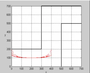
(27) Case 2: Outputs generated by FNN with algorithm 1.. Figure 7(a) Output generated by FNN with different algorithms. Case 1. Case 2 Figure 7(b) Outcome of the generated path.. 27.

(28) Figure 7(b) shows the real paths by using the two set of weighting factors obtained from different algorithms. Table 2: Comparison of errors in case 1 and case 2 Error Case 1. Case 2 Output 1 4.64×10-4. -6. 1.33×10. Output 2 3.71×10-4 From Table 2, it is obvious that the performance of FNN applied with Algorithm 2 (i.e., case 1) is more advantageous than that applied with Algorithm1 (i.e., case 2) in dealing with multiple desired outputs when the precision is strictly required.. 28.

(29) Chapter 4 Reduction of Rule Base To define a large size of rule base may not be avoided in real applications since the desired outputs usually vary case by case. Thus for generating some simple desired outputs, the efficiency is quite low due to lots of redundant rules is taken into account. Thus it is essential to extract the dominant rules from the large rule base given initially since the other rules reduce efficiency much but have no distinct effect on precision. It has been shown that after tuning the rule base by removing singular value, the error depends on the weight of the square of removed singular values σi2, which equals the magnitude of ||xi*||2. Thus the objective is to reduce the weight of removed vector. To derive the method for realize this objective, we should explore the fundamental of singular value decomposition (SVD). That is, the performance of SVD is a unitary transformation, so that the norm of FNN matrix G is conserved [9, 10], as described by the following equation: m+ p. G = ∑ xi. 2. i =1. =. m+ p. ∑ i =1. xi*. 2. (24). Where m and p denote number of rules and number of desired output respectively. It is known that by performing SVD, the dominance of the most significant vector is maximized, because it lies on the direction where the data has the most intensive distribution [9~14]. This implies that the dominance of the most significant vector increases with the correlations between the given vectors. From (24), increasing the dominance of significant vector accompanies with reducing the significance of the other ones. Thus we can obtain a trivial vector suppose that the correlations between the original vectors are highly correlated with each other. Thus the criterion for reduce the weight of removed vector xi* is to increase the value of. u xi , u d. ,. where u xi and ud represent the unit vectors of rule vectors and desired output vector respectively. Actually, the condition implies that the direction of the trivial vector is far from that of all the original vectors {x1, x2, x3 ,…, xp+m} since the original vector set has little component distributing on this direction. Thus the procedure for determining the dominant rule. 29.

(30) base can be described by the following Algorithm 3. Algorithm3: Determination of dominant rule base The FNN shown in Figure 1 has m fuzzy rules {r1(t), r2(t), …, rm(t)}.with p desired outputs {d1(t), d2(t) , …, dp(t)}. Given: Desired outputs: d1(ti), d2(ti), d3(ti),..., dp(ti) Rule base: {r1(ti), r2(ti) , …, rm(ti)}. Where ti denotes the ith sampling instant (i=1~n) Threshold of correaltion between rule and desired output: Ctr. Threshold of precsion index Ptr. Goal: Determine the dominant rule base from the given rule base for generating the specified desired output d(ti) Step 1: Compute the correlation between each normalized desired output and rule vector in the given rule base. That is, to compute the values: u ri , u dj (i = 1 ~ m , j = 1 ~ p ). The notation “u” represents the unit vector. Step 2: Find the set consists of rules rk ( k = 1, 2, u ri , u dj > C tr. m ) satisfying the following relation: ( j = 1 ~ p). Step 3: Check if the least square error (LSE) is below the preset threshold. That is: LSE < Ptr. If the above condition exists, the selected rules exactly constitute the rule base; otherwise, go to step 4 Step 4: Construct the FNN matrix G associated with the given rule vectors selected in step2 and desired output vectors, such as. 30.

(31) ⎡ d1 (t1 ) d p (t1 ) r1 (t1 ) ⎢ ⎢d1 (t2 ) d p (t2 ) r1 (t2 ) G = ⎢d1 (t3 ) d p (t3 ) r1 (t3 ) ⎢ ⎢ ⎢d1 (tn ) d p (tn ) r1 (tn ) ⎣. rs (t1 )⎤ ⎥ rs (t2 )⎥ rs (t3 )⎥ ⎥ ⎥ rs (tn )⎥⎦ n × ( p + s). Where the number rules in the rule set found in step 2 is denotes as s Step 5 Tune the selected rules by resetting the least significant p singular values of FNN matrix defined in step 4 to zeros. The tuned rule base is the desired rule base.. The above algorithm may be effective in dealing with a small group of desired outputs with high correlation, whereas it may be disadvantageous in dealing with large number of desired outputs, especially when these desired outputs are little correlated with each other. To be specific, suppose the dominant rule base for desired outputs (d1, d2, d3,…, dp ) are (R1, R2, R3,…, Rp ) respectively. It is obvious that the dominant rule base for generating all the desired outputs is quite large provided that these rule base (R1, R2, R3,…, Rp) are little in common (i.e., Ri ∩ R j. Ri or R j (i ≠ j ) ). That is, Ri << R1 ∪ R2 ∪… ∪ R p. (i = 1 ~ p ). Where Ri represents the dominant rule base corresponding to the ith desired output, and the number of total desired output is p. Consequently, the extension of rule base may be essential suppose that we want to precisely generate all the desired outputs simultaneously, however, it is time consuming for dealing with large size of rule base. Thus, when dealing with large quantity of desired outputs that are little in common, Algorithm 2 is the better choice, since the output can be precisely generated via fewer rules by applying this algorithm. Absolutely, the convention of FNN matrix should be replaced by the convention defined in Algorithm 2.. 31.

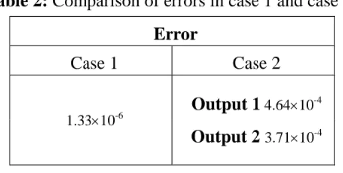
(32) Chapter 5 Illustrative Examples In this chapter, we will show the advantage of SVR algorithm in simplifying the rule base. The car navigation and system identification problems are taken as examples for illustration.. Example 1: Navigation of Model Car [1] In this example, the car will be navigated along a predefined path confined by the boundary walls. The position of car is specified by x, y, and z is the angle between the direction of cat and the horizontal axis (i.e., x axis). We set x, y, z as input variables, so that the input training data are the values of x, y and z corresponding to the position on the desired path. The criterion for defining the desired path is to prevent the car from bumping into the boundary walls. For instance, the path shown in Figure 8 is feasible among all the possible situations so that we can let it be the desired path for the car navigation.. Figure 8 A feasible path for car navigation. The output training data are obtained from sampling the values of angles at the positions next to the position (i.e., x(tk), y(tk)) where the car is located (i.e., z(tk+1)).Where tk represents the kth sampling instant. The membership functions constructing the rules of FNN are shown in Figure 9: 32.

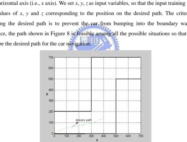
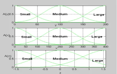
(33) Figure 9 Membership functions A(x), A(y), A(z) for generating the desired path shown in Figure 8.. We wish to utilize the FNN to generate all the desired paths with the same tuned weighting factors. The rule base obtained from the membership functions in Figure 9 is roughly derived from human feeling so that it may contain redundant rules. In the following paragraph, both of the outcomes obtained from the original rule base and that obtained from the reduced rule base will be shown Case1: Paths generated from the original rule base (twenty-seven rules). The square singular values belonging to the associated FNN matrix are listed as follows Table 3 Square of singular values of the associated FNN matrix 82.27785494343895. 0.00001985099054. 0.00000000044913. 5.24968494199168. 0.00001856865610. 0.00000000025627. 1.67374902813030. 0.00000539945881. 0.00000000016226. 0.25320269522639. 0.00000419872013. 0.00000000000427. 0.04431626435280. 0.00000028517688. 0.00000000000339. 0.01542454876520. 0.00000010746623. 0.00000000000018. 0.00200855604145. 0.00000006766903. 0.00000000000014. 0.00055397135821. 0.00000005653205. 0.00000000000000. 0.00019773748329. 0.00000000146113. 0.00016438555941. 0.00000000065496. Table 3 demonstrates the existence of numerous trivial singular values, which have nominal 33.

(34) effect on total vector set. This implies that the performance of FNN would be satisfying using the given rule base. Table 4 Rule base defined from membership functions in Figure 9. Input variable x. y. z. 0. 1. 2. 1. 0. 0. 0. 2. 0. 0. 1. 3. 0. 0. 2. 4. 0. 1. 0. 5. 0. 1. 1. 6. 0. 1. 2. 7. 0. 2. 0. 8. 0. 2. 1. 9. 0. 2. 2. 10. 1. 0. 0. 11. 1. 0. 1. 12. 1. 0. 2. 13. 1. 1. 0. 14. 1. 1. 1. 15. 1. 1. 2. 16. 1. 2. 0. 17. 1. 2. 1. 18. 1. 2. 2. 19. 2. 0. 0. 20. 2. 0. 1. 21. 2. 0. 2. 22. 2. 1. 0. 23. 2. 1. 1. 24. 2. 1. 2. 25. 2. 2. 0. 26. 2. 2. 1. 27. 2. 2. 2. Variable number Rule number. 34.

(35) Where 0, 1, 2 represent small, medium, large respectively. Correspondingly, Aij represents the jth (j = 0~2) membership function associated with ith (i = 0~2) input variable. The rules are products of membership functions defined in Figure 9. Three membership functions are set for each input variable as shown in Figure 9. Thus we have 27 rules, which are defined in Table 4. The weighting factor associated each rule defined in Table 4 are listed in Table 5. Table 5 Weighting factor associated with each rule Rule 1~9. Rule 10~18. Rule19~27. -0.75571907837368 0.73363731354769 -3.88755820107623 3.64928526212313 -0.73617434143575 -1.44428673043869 -1.30427508117294 0.38102407422188 -1.07923508586419 0.03623954020896. 0.01399107323513. 0.10170459483365. 0.00178423256134 -0.02049810344030 -0.04851905055454 0.05897749993184. 0.02514866212161 -0.03263706582737. -3.15560891193539 -1.50142999664931 0.24361646489375 -0.84900405057501 1.67238543093995. 1.44908269164601. 3.14336213428962 -1.63329345274953 -2.35704795920322. The output generated by FNN is shown in the following figure:. Figure 10. Paths of different cases generated by 27 rules Case1: Path originating from the origin. Case2: Path originating from y = 80 Case3 Path originating from y =100. 35.

(36) The result shown in Figure 10 shows that the paths with different initial conditions are successfully generated from the FNN with the same weighting factor set. The error between the desired output and actual output generated from twenty-seven rules are trivial (i.e., 8.65×10-5). However, the efficiency may not be satisfying since we have set large quantity of rules in the FNN. Thus, we may wish to accomplish the navigation task by generating the desired output via fewer rules with slightly reduction of precision so that the generating efficiency can be much increased. Consequently we will adopt Agorithm3 to extract the dominant rule base. The overall procedure is listed as follows:. Case2: Paths generated from the reduced rule base. Let Threshold of precision index (Ptr) = 10-3, Threshold of correlation (Ctr) = 0.93 The correlations between desired output and each rule are listed as follows:. Rule 1~ Rule 9 0.8738. 0.8811. 0.9058. 0.9161. 0.9258. 0.9198. 0.9306 0.9385. 0.8596 0.8612. 0.8729. 0.8845. 0.8754. 0.8868. 0.8992 0.9111. 0.9216 0.9316. 0.9203. 0.9293 0.9374. 0.8876. Rule 10~ Rule 18 0.8401. 0.8500. 0.8977. Rule 19~ Rule 27 0.8833. 0.8916. The correlations corresponding to rule 8, 9, 24, 27 are larger than the preset threshold (Ctr) so that they will be selected. The least square error (LSE) = 9.87×10-4 < Ptr The above data shows that the selected rules are sufficient to satisfy the precision bound. Therefore, we can let the rule base be the set of the selected four rules. The membership functions for constructing them are listed as follows: Rule 8: A00, A11, A21.. 36.

(37) Rule 9: A00, A11, A22. Rule 24: A22, A11, A22. Rule 27: A02, A12, A22. Thus all the membership functions constructing these rules are: A00, A02, A11, A12, A21, A22 The fact shows that three membership functions can be eliminated since only six of the predefined nine membership functions are utilized. The redundant membership functions to be eliminated are A01, A10, A20. The weighting factor set corresponding to the rule base is: -1.9119. 4.2080. -0.0002. -0.9458. The following figure shows the performance of FNN in dealing with the car navigation problems with smaller size of rule base.. Figure 11 Paths in three different cases are generated by the FNN with four rules. Case1: Path originating from the origin. Case2: Path originating from y = 80 Case3: Path originating from y =100. The result shows that the desired path can be successfully generated using only a few rules. Next, we will try to generate the paths originating from both the upper corner and bottom corner via the same reduced rule base, as shown in the following figure:. 37.

(38) Figure 12: Two general cases of navigated paths.. In order to cope with all the possible situations, the reduced rule base should be properly tuned such that we can always obtain the satisfying result in different situations by the FNN. Therefore, we have to retrieval the training data from all the valid paths. The corresponding weighting factor set obtained from least mean square method is: -1.3375 2.9379 -0.0002 -0.6561. The outcome is shown in the following figure:. Figure13: (a) The approximated paths in different cases generated by the FNN without tuning the rule base by regulating singular values. Case 1: path originating from (0,177). Case 2: path originating from (0,130). Case 3: path originating from (0,30). Case 4: path originating from (0,75).. 38.

(39) Figure13: (b) The approximated paths in different cases generated by the FNN with tuning the rule base by regulating singular values. Case 1: path originating from (0,177). Case 2: path originating from (0,130). Case 3: path originating from (0,30). Case 4: path originating from (0,75).. In comparison with Figure 13(a) and (b), the tuning approach is not essential if the precision is not strictly required. However, for some special cases, the error will be tremendous suppose that the desired paths are generated from the rule base without tuning by regulating singular values, such as the ones shown in Figuer14:. Figure 14: Two special cases of navigated paths generated by the FNN. Case 1: path originating from (100,200). Case 2: path originating from (300,0). The paths shown with dot lines are generated from the rule base without tuning by regulating singular values, while the paths shown with solid lines are generated from the rule base tuned by regulating singular values.. The outcome shows that the FNN obviously fail in generating the desired output via the. 39.

(40) originally given rule base owing to the conditions specified by the desired output and rule base quite mismatch with each other. That is, all rules defined in the rule base are little correlated with the desired output, as shown in the following table: Table 6 Correlations between rules and desired output Rule 1. 0.0064. Rule 2. 0.0098. Rule 3. 0.0079. Rule 4. 0.0104. Under this circumstance, the vector space where desired output vector belongs is close to the null space of the vector space spanned by rule base. Thus, the least square error (LSE) is close to the square norm of desired output vector, (i.e., ||x1||2). However, after tuning the mismatched rule base via regulating singular value, the error exactly depends on the projection of desired output vector (i.e., x1) on the removed vector (i.e., xm+1*). We name the error for regulating error (RE). Apparently, RE is much smaller than LSE since RE is only a small proportion of ||x1||2. That is: x1. 2. = ( Cx1* ) + ( Cx2* ) + 2. 2. + ( Cxm* +1 ). 2. Where ( Cxi* ) represents the projection of x1 on xi* (i =1~m+1), and 2. ( Cx ). 2 * m +1. = RE. We can examine the fact from the error between the generated paths of FNN and desired paths (i.e., RE = 6.21×10-5, LSE = 0.89). The result shows that the performance of FNN is indeed improved since both the error and rule base can be kept small. The outcomes obtained from the tuned rule base and that obtained from the rule base without tuning are compared in the following figure:. 40.

(41) 5.00E-04 4.00E-04 Regulating 3.00E-04 Error 2.00E-04 (RE) 1.00E-04 0.00E+00 0.001. 0.01. 0.1. 1. Least Square Error(LSE). Figure 15 Advantage of tuning the rule base. The data are relevant to the cases shown in Figure 13 and 14. The increase of RE is quite smaller compared with that of LSE, which depends on the correlation between rules and desired output.. Figure 15 shows that the precision can be well maintained provided that the output is generated from the tuned rule base. Thus the rule base is certainly kept small since we only have to modify the given rule base without setting new rules for generating the output that is little correlated with the original rule base.. Example 2: System identification of a plant model [7]. In this example, the system of a first-order nonlinear plant is going to be identified. The plant to be identified is of the following form:. y (k + 1) = g[ y (k ), u (k )] Where the unknown function has the following nonlinear form: g ( x1 , x2 ) =. x1 + x23 1 + x2 2. and u(k) = sin (2πk/25) + sin(2πk/10). The series-parallel identification model is: y ( k + 1) =. fˆ [ y ( k ), u ( k )]. Where fˆ is in the form of output of fuzzy neural network with two fuzzy input variables whose Gaussian membership functions are defined in the following Table 7:. 41.

(42) Table 7 Center and width for fuzzy sets of x1. Center and width for fuzzy sets of x2. Center 0.5 0 3 5. Center -2 0 1 2. A00 A01 A02 A03. Width 0.5 0.3 0.4 0.6. A10 A11 A12 A13. Width 0.6 0.6 0.6 0.6. Case 1: System identified by 16 rules.. We define training space as –100< k <100 and retrieval one thousand training data points from the defined training space. The obtained singular values of the associated singular values are listed as follows: Table 8 Singular values of the matrix consists of rules and desired output 6.19322235099177. 0.00000000039161. 0.00000000000042. 0.05865327981720. 0.00000000022078. 0.00000000000014. 0.00000617453351. 0.00000000016806. 0.00000000000009. 0.00000000750532. 0.00000000000617. 0.00000000000000. 0.00000000163361. 0.00000000000520. 0.00000000000000. 0.00000000054607. 0.00000000000213. The high redundancy of singular values shown in Table 8 demonstrates that too many redundant rules are set for identifying the system. This implies that only a few rules among the given rule set are essential for identifying the plant model. Thus will adopt Algorithm 3 to extract the dominant rules.. Case 2: System identified by reduced rule base.. We apply Algorithm 3 to determine the dominant rules for identifying the system such that the rule base can be reduced as the set consists of these dominant rules. The procedure is listed as follows. Let. 42.

(43) Threshold of precision index (Ptr) = 10-3 Threshold of correlation (Ctr) = 0.06. The correlations between the desired output and each rule are listed as follows: Rule1 ~Rule8 -0.2848. -0.2621. -0.2493 -0.2414. -0.0123. 0.0014. 0.0108. 0.0116. 0.0629. -0.0315. 0.4037. 0.3858. 0.3714. Rule9 ~Rule16 -0.0139. 0.0355. 0.0623. The marked values corresponding to rule 11, 14, 15, 16 are larger than the preset threshold (Ctr). Thus rule 11, 14, 15, 16 will be selected. The membership functions for constructing them are listed as follows: Rule 11: A02, A13. Rule 14: A03, A11. Rule 15: A03, A12. Rule 16: A03, A13. Thus all the membership functions for constructing these rules are: A02, A03, A11, A12, A13,. The fact shows that three membership functions can be eliminated since only five of the predefined eight membership functions are utilized. The redundant membership functions to be eliminated are A00, A01, A10. The least square error (LSE) = 9.68×10-3 > Ptr Due to the error exceeds the preset precision bound, we have to tune the selected rules by removing the trivial singular value of the associated FNN matrix. The square of singular values of the FNN matrix are listed as follows: 5.34295850306414. 0.00026015790148. 0.00000007638967. 0.00000012271620. 0.0000000044133. After removing the least significant singular value, the obtained weighting factor set corresponding to the rule base is: 0.000424 -0.004345. 0.289796. 2.018651. The approximation of system output and the real system output are shown as follows:. 43.

(44) Figure 16. Case2: System identified by 4 rules. * : generated output of FNN.. _: system output. After tuning the rule base, the least square error is 3.38×10-7 which is quite smaller than the preset threshold. Next, we will replace the original sinusoidal input by the step input to see if the output can match the step response of this system. The result is shown in the following figure:. Figure 17 Step response of the system identified by four rules. Dashed line: generated output of FNN. Solid line: desired output. The least square error is 9.38×10-4. The result shows that the theoretical system output is much close to the generated output of FNN. The phenomenon confirms that the system performance can be replaced by the FNN with a simpler rule base.. 44.

(45) Conclusion The methodology for enhancing the fuzzy neural network in coping with various relations between the fuzzy inputs and outputs has been presented in this paper. The result shows that the FNN is able to precisely generate the desired output in many complicate situations via a small size of rule base that is well tuned by regulating singular values. Because the rule base is kept small, the generating efficiency is much higher so that the FNN is able to efficiently confront a variety of complicate situations in the real world applications. In addition, to update the weighting factor set becomes an easier task so that the FNN may also be applied in dealing with the situation that occurs instantly. To sum up, regulating singular values approach enables FNN to deal with complicate inputs and outputs relations more efficiently, as illustrated in this paper.. 45.

(46) Reference [1] C. H. Wang, W. Y. Wang, and T. T. Lee, “Fuzzy B-Spline membership function (BMF) and its application in fuzzy-neural control,” IEEE Trans. System, Man, Cybernetics”, Vol.25, pp.841-851, 1995. [2] T. Sudkamp, A Knapp, and J. Knapp, “Model generation by domain refinement and rule reduction,” IEEE Trans. System, Man, Cybernetics – Part B: Cybernetics”, Vol.33, Issue.1. pp.45-55, Feb.2003. [3] R. Thawonmas, and S. Abe, “A novel approach to vector selection based on analysis of class regions”, IEEE Trans. System, Man, Cybernetics– Part B: Cybernetics, Vol.27, No. 2, pp. 196-207, April 1997. [4] Y. Yam, P.Baranyi, and C. T. Yang, “Reduction of fuzzy rule base via singular value decomposition,” IEEE Trans. Fuzzy System, Vol.7, pp.120-132, April 1999. [5] C. W. Tao, “A Reduction Approach for Fuzzy Rule Bases of Fuzzy Controllers,” IEEE Trans. System, Man, Cybernetics - part B: Cybernetics, Vol. 32, pp, 1-7, 2002.. [6] Simon Haykin, “Neural network”, Hamilton, Ontario, Canada: Prentice Hall, 2nd ed, 1999. [7] C. H Wang, H. Lei, and C. T. Lin, “Dynamical optimal learning rates of a certain class of fuzzy neural network and its application with genetic algorithm,” IEEE Trans. System, Man, Cybernetics – Part B: Cybernetics, Vol. 3, pp. 467-475, June 2001.. [8] Edwin K.P Chong, and Stanislaw H. Zak, “An introduction to optimization” John Wiley, 2001. [9] L. I. Smith, “A tutorial on principal component analysis”, handout. February 26, 2002. [10] K .I. Diamantaras and S. Y Kung, “Principal Component Neural Networks Theory and Applications” John Wiley & Sons Inc. 1996. [11] Agresti Alan,“Categorical data analysis” John Wiley & Sons. 1990 [12] Lewis Paul J,“Multivariate data analysis in industrial practice＂ Research Studies Press 1982. [13] Pavlidis, Theodosios, T. Pavlidis,“Structural pattern recognition＂Springer-Verlag, 1977 [14] Batchelor, Bruce G., edited by Bruce G.. Batchelor.“Pattern recognition: idea in practice, Plenum Press, 1978. 46.

(47)