A Sliding Mode Current Control Scheme for
PWM Brushless DC Motor Drives
Jessen Chen and Pei-Chong Tang
Abstract—This paper proposes a sliding mode current control scheme for pulsewidth modulation (PWM) brushless dc motor drives. An improved “equivalent control” method is used in this scheme. A simple algorithm is proposed that differs from the original equivalent control method, which requires extensive calculation to estimate the load parameters. This algorithm can be implemented using logic circuits. Moreover, using autotuning, the proposed algorithm can be applied without load information. An operating principle for the power stage switching devices called single-side firing is also proposed. Single-side firing solves the dead-time problem, allowing the PWM frequency to be increased and the sampling rate to be raised. This paper explains the current control algorithm, single-side firing principle, and implementation of the proposed scheme in detail. Simulations and experimental results are given to show the validity of this scheme. Index Terms— Brushless dc motor, current control, sliding mode.
NOMENCLATURE AND CONVENTIONS
Armature voltage and current. Motor inductance and resistance. Back electromotive force (emf). Rotor velocity.
Boldface Vectors/matrices.
Superscript Set points.
Superscript Estimated values.
Subscript phases.
Subscript Error.
I. INTRODUCTION
C
URRENT-CONTROLLED pulsewidth modulation(PWM) inverters are extensively used in high-performance servo drives. For a brushless dc motor, stator current is directly related to developed torque, so current controllers play important roles in these drives. Among the many current control techniques, three conventional methods are used most—hysteresis control, ramp-comparison control, and predictive control. Hysteresis control is the most extensively used method. It responds quickly, requires no load information, and is easy to implement. However, hysteresis current controllers have several disadvantages. The steady-state current ripples are relatively high. Switching frequencies vary during operation, leading to irregular inverter operation and generating PWM noise [1]–[3]. The
Manuscript received August 26, 1996; revised June 29, 1998. Recom-mended by Associate Editor, L. Xu.
The authors are with the National Chiao Tung University, Hsinchu, Taiwan, R.O.C.
Publisher Item Identifier S 0885-8993(99)01821-9.
main advantage of the ramp-comparison technique is that the switches operate at fixed frequencies. However, problems include appreciable phase lags and magnitude errors at high frequencies, and complicated PLL circuits are required to overcome these problems. Predictive control gives good performance in terms of response time and accuracy, but it requires extensive calculation and accurate load information [1], [3]. Recently, many current control techniques have been developed—sliding mode technique is one of them. Broad bandwidth and robustness to parameter variation are among its advantages. Although implementation of sliding mode control implies high-frequency switching activity, this does not cause any difficulties because “on–off” operation is very natural for a PWM amplifier [4]. Current control using the sliding mode technique was proposed in [4] and [5]. In [4] and [5], adaptive parameter estimation was used to estimate load parameters. The disadvantage of this approach is that the estimation requires extensive calculation.
This paper proposes a sliding mode current control scheme that uses an improved “equivalent control” method. Unlike the original equivalent control method, which requires extensive calculation to estimate load parameters, our simple algorithm does not require complicated computations. It is easy to imple-ment this algorithm using logic circuits, and this paper explains implementation using a field-programmable gate array (FPGA) chip. Moreover, autotuning allows the proposed algorithm to be applied without load information.
The proposed algorithm requires a high sampling rate to achieve fast accurate responses, however, the sampling rate is limited by the PWM frequency. To solve this problem, an operating principle for the switching devices called single-side firing is proposed. With single-side firing, only one side (the upper or lower leg) is turned on during each PWM cycle. The dead time needed to prevent short circuiting is no longer necessary. Without the dead-time limitation, PWM frequencies can be increased and sampling rates can be raised.
This paper explains the sliding mode current control scheme in detail. The current control algorithm is explained in Section I. A dc motor model is first used to introduce the algorithm and then the results are extended to a brushless dc motor. Simulation results involving a dc motor and a brushless dc motor are presented, and an autotuning method is proposed. In Section II, the single-side firing principle is described, and a comparison of single-side firing with a conventional method is presented. In Section III, FPGA implementation is introduced. Experimental results are given in Section IV, and conclusions are drawn in Section V.
II. SLIDING MODE CURRENTCONTROL
In this section, the control algorithm is deduced, a dc motor model is considered first, and then the results are extended to a brushless dc motor. With certain modifications, the control algorithm for a dc motor can be applied to each of the three phases of a brushless dc motor.
A. Sliding Mode Current Control for DC Motors
The voltage–current equation for a dc motor is expressed as follows:
(1) In (1), is the control input. The set-point tracking problem can be transformed into the stabilization problem for the system in error form. The sliding surface is defined by the
scalar equation , where
(2) The sliding mode exists if
(3) To satisfy (3), an “equivalent control” method is used. The control input is expressed as
(4) Substituting (4) into (3), the sliding condition becomes
(5) where
and (6)
(7) In (4), can be interpreted as the approximation of the
continuous control law that would remain , and
is the discontinuous part which helps to satisfy the sliding condition in the presence of parameter uncertainty [6], [8]. Deriving requires estimating motor parameters. However, this estimation requires considerable calculation, thus, the equivalent control method is difficult to implement. This paper proposes a simple algorithm based on the equivalent control method. This algorithm does not require any parameter estimation and can be implemented by logic circuits. To deduce the algorithm, we modify the control law to the following form:
(8) (9)
In (9), is derived using integration. Under ideal conditions, the should be of the following form:
(10)
Thus, if , an exact control voltage can be
derived, i.e., In (10), the term is
contributed by the variation in current, and the term is contributed by the variation in rotor speed. Since the velocity loop response is relatively slow when compared with the
current loop response, is much larger than and
can be ignored, which leads to
(11)
where can be derived by substituting (11)
into (9).
The estimated control voltage derived from (9) and (11) is not exact because the variations in back emf are not considered, but as long as is such that the sliding condition (5) is satisfied, the tracking error will converge to zero.
The method proposed above requires the motor-parameter information. However, under the condition that is unknown, let
and (12)
It will be shown that as long as and satisfy certain conditions, the control algorithm in (8) and (9) will still work effectively. Assuming that a step command is applied at , the value of is such that the current response matches the following specifications:
1) sliding condition (5) can be satisfied;
2) response must reach the set point within a given time The satisfaction of the sliding condition can be checked in two stages. During the time , will not change its sign. The sliding condition can be checked by substituting (7)–(9) and (12) into (5). If is ignored, the sliding condition becomes
(13)
If , by solving the differential equation (1),
(13) becomes
(14)
In (14), the term is negative, thus, when
, the sliding condition (5) will be satisfied for any value. The satisfaction of the sliding condition ensures that the current error always decreases or remains at zero, and will never have the chance to change its sign. However, due to the imperfection of the switching devices in practice, will change its sign when the current response reaches the set point. At this moment, the sliding condition will be satisfied if
(15)
From (15), the upper bound of is derived as follows: (16)
The spec. of response time implies
(17)
Let From (17), the lower bound of is
derived as follows:
(18)
The upper and lower bounds of can be derived from (16) and (18) if
(19)
From (19), letting , the upper bound of can
be derived as follows:
(20) As long as (20) is satisfied and satisfies the following:
(21)
the current response will match the two specifications. The control law in (8) and (9) can be transformed into the discrete form
(22) (23)
where and is the sampling period. In (23),
the control law is such that will be changed only when because in the steady state, if
and , will change its sign during every
sampling period, thus, the value of must not be changed. Implementation is easier if (22) and (23) are transformed into the following form:
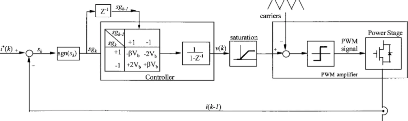
if if
(24) The current controller architecture is shown in Fig. 1. The controller consists of a lookup table and an integrator. The lookup table is constructed according to the signs of and The integral value is determined according to the lookup table. The output of the controller passes through a saturation function block because the dc bus voltage is limited. The output of the saturation function is then sent to a PWM amplifier.
The dc motor simulation result is provided to verify this sliding mode current control scheme. The parameters for
simulation were and mH, and the dc bus
voltage was 150 V: A, , and
s. The response speed specification was given as s. The upper bound of can be derived from (20)
Letting , we have V. The bound on
can be derived from (21), and it is
Let , thus, The result is shown in
Fig. 2.
B. Sliding Mode Current Control for Brushless DC Motors The brushless dc motor may be modeled as follows:
(25) where
where is the mutual inductance and is the neutral-point voltage. With a three-phase balanced load, can be expressed as
(26)
From (25), -phase voltage–current equation can be expressed as
(27) where
and (28)
(29) Assuming that when the rotor speed is constant, a constant phase lag exists between the current reference and the emf
(30) (31)
(32) where as the peak emf value and as the peak current-reference value. If the motor is not operating under field-weakening control, the emf can be assumed to be in phase with the current reference. In general, can be expressed in the following form:
Fig. 1. The proposed sliding mode current controller architecture.
Fig. 2. DC motor simulation result.
where
and (34)
(35) For a cascade control structure, the current reference is the velocity-loop output passing through a sample-and-hold, and it can be treated as a sequence of step changes. If the velocity-loop sampling time is much longer than the time required for the current step response to reach the set point, (27) can be written as
(36) where
and (37)
(38) For the system represented by (36), the control law in (8) and (9) is still effective, but the definition of must be changed to the following form:
(39)
Fig. 3. Brushless dc motor simulation result.
Fig. 4. The conventional switching-device operation.
Thus, if the following is satisfied:
(40) and (39) can be written as
(41) The control law is the same as that for the dc motor if we let (42) Thus, each of the three phases can be controlled by (8), (9), and (12). The bound for and can still be derived in the
(a) (b) Fig. 5. (a) Single-side firing with positive current command. (b) Single-side firing with negative current command.
same manner. To satisfy (40), let
and (43)
(44) From (8), (9), (43), and (44), we have
(45) With (43) and (44) satisfied, the same control algorithm used for a dc motor can also be used for each of the three phases.
A simulation result is shown in Fig. 3. The motor param-eters are the same as those for the dc motor, and mutual inductance is ignored. The emf constant for the brushless dc motor was 0.46 V rad/s. A 10-Hz three-phase current reference was given with a peak value of 2 A, and the current reference was sent to a sample-and-hold to generate a step sequence. The operating frequency of the sample-and-hold was 1 kHz. The phase lag between the emf and current reference was zero. The response speed specification was given as follows: at
A, s. The sampling time was 0.000 025 s.
From (34) and (35), we have and Thus,
according to (37), (38), and (42), The bound for
can be derived from (20), and it is
Let , and the bound for can be derived from (21),
which is
Let and The result is shown in Fig. 3.
Simulation results in Figs. 2 and 3 show the validity of the sliding mode control algorithm, however, motor parameters are required to calculate the bounds for and The brushless dc motor case is even more complicated because with different and in (46), different bounds for and must be calculated. However, when this algorithm is used in practice, with only two parameters to tune, an on-line autotuning procedure can be applied when the motor parameters are unknown. Since when neither (34) nor (35) is satisfied, either the response speed will not match the specification or the current response will
Fig. 6. Three-phase operation for the single-side firing principle with pos-itive u-phase current command and negative v-phase and w-phase current commands.
produce obvious overshoot. and can be tuned according to the following rules.
1) If the response is slow (the “ ” spec. cannot be sat-isfied), but no overshoot occurs, a larger must be applied.
2) If the response is slow and overshoot occurs, a larger must be applied.
3) If the response is fast enough (the “ ” spec. is satisfied) and no overshoot occurs, a smaller must be applied. 4) If the response is fast enough, but overshoot occurs, a
smaller must be applied.
Using the rule-based autotuning procedures, an and versus and table can be constructed for brushless dc motors. Once the table has been constructed, every time a step command is applied, and can be set according to the table, and the table contents can be updated on line according to the rules. The rule-based autotuning procedure is very suitable for using the fuzzy control technique, however, this is beyond the scope of this paper. In Section IV, a simple autotuning method based on the rules is presented, and the reported experimental result is good.
III. THESINGLE-SIDEFIRING PRINCIPLE
The proposed sliding mode current controller requires a high sampling rate to achieve high performance. With a high sam-pling rate, the current controller can generate high-frequency switching activity, which leads to low-current ripples in the steady state and fast transient dynamics. The sampling rate is limited by two main factors: one is the control algorithm execution time, and the other is the PWM frequency. The control algorithm for the proposed current controller can be implemented using logic circuits yielding execution speeds
Fig. 7. Hardware block diagram of the servo drive.
Fig. 8. Block diagram of the FPGA internal circuits.
fast enough for even high sampling rates. However, raising the sampling rate depends on increasing PWM frequency. The PWM frequency is limited mainly by the characteristics of the switching devices and the dead time. Recently, many high-speed devices, such as insulated gate bipolar transistors (IGBT’s) and MOSFET’s, have been developed, however, they still require switching dead time around 1–2 ms. The existence of dead time is an obstruction to raise the PWM frequency. Moreover, if not properly compensated for, it will lead to serious problems, such as waveform distortion and increased
torque ripples [7]. In order to raise the sampling rate, a new switching device operating principle called single-side firing is presented to solve the dead-time problem and raise the PWM frequency.
Along with the introduction of the single-side firing princi-ple, the conventional method is reviewed for comparison. A conventional switching-device operation is shown in Fig. 4. The PWM signal and the inverse PWM signal are fed to switches and , respectively. During every PWM cycle, and are both turned on and off once. In order to
Fig. 9. Block diagram of the current controller.
(a) (b)
(c)
Fig. 10. The current step response. (a) K1 = 1 and K2 = 30: (b) K1 = 4 and K2 = 120: (c) K1 = 4 and K2 = 120 in transient, but the
values of K1 and K2 are decreased in every sampling period.
TABLE I
protect and from the risk of being short circuited, a dead time is inserted into the PWM signals.
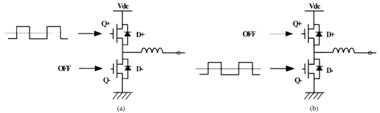
The single-side firing principle is similar to the approach used in [9]. In [9], an one-switch-active topology was pre-sented for an electronically commutated motor (ECM) drive with trapezoidal current excitation. The concept is that only one switch is gated “on” during braking. In this paper, the similar idea is extended to the sinusoidal phase current con-dition and applied during motoring. The proposed single-side firing principle is shown in Fig. 5. In Fig. 5(a), the current command is positive, and the PWM signal is fed only to
(a) (b)
(c)
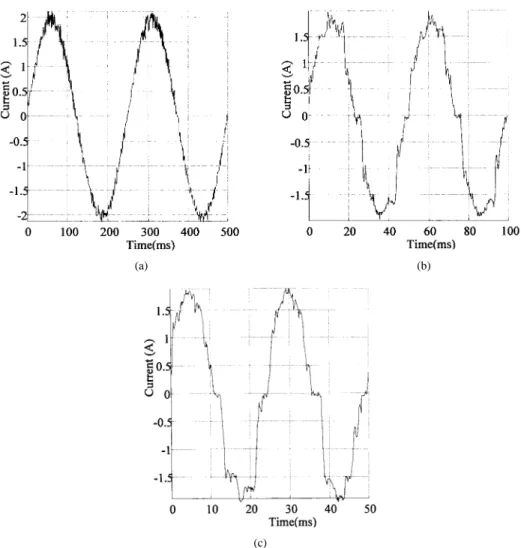
Fig. 11. The sinusoidal current waveforms with K1 = 1 and K2 = 10: (a) 4 Hz. (b) 20 Hz. (c) 40 Hz.
, with always off. During a PWM cycle, current flows
through when is on and flows through the flywheel
diode when is off. In Fig. 5(b), on the other hand, the current command is negative, and the PWM signal is fed only to , with always off. Current flows through when is on and flows through the flywheel diode when is off. Using this principle, dead time is removed because and will never have a chance of being turned on simultaneously, except for the instant during which the current-command sign is being changed. Without the dead-time limitation, the switching frequency can be increased, and because only one switch is active during each PWM cycle, the switching loss is half that of conventional methods used under the same switching frequency conditions.
One example of the three-phase operation for the single-side firing principle is shown in Fig. 6. The polarity of -phase current command is positive, and the polarities of the and phases are negative. The -phase PWM signal is fed only to the upper switch, and the PWM signals of and phases are fed only to the lower switches.
One thing about the single-side firing principle must be pointed out: without a connection to the dc bus or ground at all times, the coils will be floating when and are both off and the phase current decays to zero. At this time, the coil’s terminal voltage is undefined and the linearity between
the PWM duty cycle and the control voltage is lost. However, the undefined coil voltage will not affect the performance of the proposed controller because the proposed control law is nonlinear, and PWM duty cycles are not determined by coil voltage information.
IV. HARDWARE
A hardware block diagram of the servo drive is shown in Fig. 7. The hardware consists of an Intel 80 188 central processing unit (CPU), digital–analog (D/A) converters, FPGA chip, comparator circuits, and power stage.
A cascaded control structure is used. The CPU takes care of the outer position loop and velocity loop. The inner current control loop is implemented by the FPGA chip. When current references are sent to the D/A converters by the CPU, the comparator circuit compares the current command and the feedback current signal and sends the results to the FPGA. The current control algorithm is executed in the FPGA. The encoder feedback signals are also sent to the FPGA, where they are transformed into position feedback information. The switching devices used in the power stages are MOSFET’s.
Instead of using a popular digital signal processor (DSP) chip or a microcontroller, an AT&T ORCA 2C04 FPGA is used to implement the current control algorithm because it has
(a) (b)
(c)
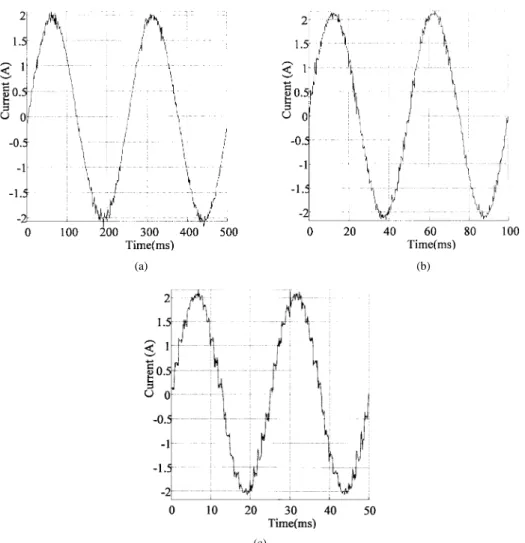
Fig. 12. The sinusoidal current waveforms. (a) 4 Hz, with K1 = 12:8 and K2 = 72: (b) 20 Hz, with K1 = 5:3 and K2 = 46: (c) 40 Hz,
with K1 = 3:9 and K2 = 47:
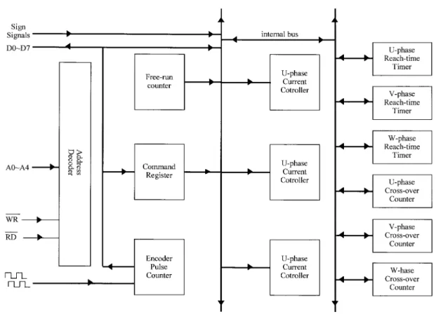
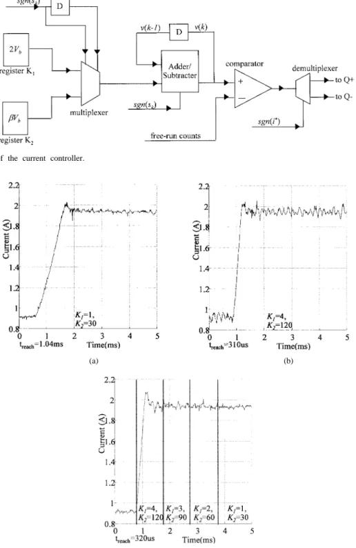
the advantages of high speed, high reliability, and high density. A block diagram of the FPGA internal circuitry is shown in Fig. 8. There is an address decoder, encoder pulse counter, command register, status register, free-run counter, three-phase reach-time timers, three-three-phase chattering counters, and three-phase current controllers. The address decoder provides all internal register-select signals; the encoder pulse counter receives the encoder feedback signals and transforms the signals into the rotor position information; the command register stores polarity information about three-phase current references which written by the CPU; the free-run counter generates the PWM carriers; and the three-phase reach-time timers and the chattering counters detect the reach time and the chattering frequency, respectively, both necessary for the autotuning procedure. The three-phase current controllers are the most important parts of the FPGA internal circuits. The control law (24) is executed by the current controller for each phase. A block diagram of each current controller is shown in Fig. 9. The current controller consists of two reg-isters, an adder/subtracter, multiplexer, demultiplexer, digital comparator, and two d-type flip flops. The registers are used to store the terms and in (24), and their resolutions are 256. The multiplexer is used to choose between and
according and , and the output of this
multiplexer is sent to the adder/subtracter. The output of the adder/subtracter is the term in (24), which is sent to a
-type flip flop to generate , and is fed back to
the adder/subtracter. The resolution of is 256, and is compared with the free-run counts to generate the PWM signals. Since single-side firing is used, the PWM signals are fed to the upper switch or the lower, as determined by the current reference polarity.
V. EXPERIMENTAL RESULTS
A 400-W brushless dc motor with a brake was used for ex-perimentation. The parameters for the brushless dc motor were the same as those used in simulation. The PWM frequency was 20 kHz, and with the centralized PWM waveforms, the sam-pling rate of the current loop can be twice the PWM frequency. Step responses and sinusoidal waveforms are presented in this section.
A. Step Response
For a cascade control structure, current reference is the output of the velocity loop. A sinusoidal current reference can be treated as a sequence of step changes. Showing the step responses is a good way to verify the proposed scheme.
In Fig. 10, current references are given to three-phase current controllers with the rotor locked by the brake. The step change of -phase current is 1 A, and the step changes of -phase and
-phase current are 0.5 A. The current step responses of
phase are shown. Letting and
, the responses are captured with different and values. Comparing the results in Fig. 10(a) and (b), it is obvious that with a larger , the step response in (b) is faster, however, higher steady-state current ripples occur. To solve the tradeoff problem, an alternative method is used in Fig. 10(c). In order to give a fast response, a larger is applied in transient, and the value of is decreased gradually in steady state to reduce the steady-state current ripples. It is shown in Fig. 10(c) that the transient response is still fast ( s), and the steady-state ripples are reduced gradually.
B. Sinusoidal Current Waveforms
To capture the sinusoidal current waveforms, the motor was run in velocity-control mode with a constant load. The sam-pling rate of the velocity loop was 1 kHz. A simple rule-based autotuning method stated in Section I was used. In Section I, the control parameters are tuned according to reach time and overshoot information. However, the detection of overshoot re-quires analog–digital (A/D) converters. In order to simplify the hardware design, chattering frequency information was substi-tuted for overshoot, thus, the A/D converters can be omitted.
When the response reaches the set point, since the switching is not instantaneous, and this leads to chattering. Chattering frequency carries very useful information. For example, a high-chattering voltage results in a high-chattering fre-quency, and this also leads to high-steady-state current ripples. However, a low-chattering voltage results in a low-chattering frequency, this also leads to slow response and long settling time.
By defining as the chattering index and as
the reach-time index, the autotuning method is described as follows.
1) If the reach time and the chattering frequency
: .
2) If the reach time and the chattering frequency
: .
3) If the reach time and the chattering frequency
: .
4) If the reach time and the chattering frequency :
where and are constants.
The autotuning procedure was executed every 0.5 s ac-cording to the average reach time and chattering frequency information for the 0.5-s period. The response specification
was given: at A, the reach-time index
s and the chattering index kHz. For
, and the initial conditions for and
were , and and were tuned
with a different rotor frequency. The result of the autotuning
procedure is shown in Table I. A and versus rotor
frequency table was constructed at 4-Hz intervals.
The current waveforms captured with the initial and value applied are shown in Fig. 11(a)–(c). The current waveforms captured with the tuned and value applied are shown in Fig. 12(a)–(c). It is obvious that the current waveforms are improved after the autotuning procedure. The improvement is very conspicuous when the rotor frequency is high.
The experimental results show the effectiveness of the pro-posed scheme. However, since the sinusoidal current reference is composed of the step commands, the higher frequency waveform show deterioration.
VI. CONCLUSION
A sliding mode current control scheme for brushless dc motors is proposed in this paper. It has been shown that the control algorithm requires no complicated computation and can be implemented using logic circuits. With a simple autotuning procedure, the proposed algorithm can be applied without load information. A single-side firing operating prin-ciple for the power stage switching devices is also proposed, which helps in solving the dead-time problem. Without the dead-time limitation, the PWM frequency and the sampling rate can be raised. The experimental results show the validity of this scheme.
REFERENCES
[1] L. Malesani and P. Tenti, “A novel hysteresis control for current controlled VSI PWM inverters with constant modulation frequency,”
IEEE Trans. Ind. Applicat., vol. 26, pp. 88–93, Jan. 1990.
[2] D. M. Brod and D. W. Novotny, “Current control of VSI-PWM invert-ers,” IEEE Trans. Ind. Applicat., vol. IA-21, pp. 562–570, May/June 1985.
[3] H. Le-Huy and L. A. Dessaint, “An adaptive current control scheme for PWM synchronous motor drives: Analysis and simulation,” IEEE
Trans. Power Electron., vol. 4, pp. 486–495, Oct. 1989.
[4] V. I. Utkin “Sliding mode control design principles and applications to electric drives,” IEEE Trans. Ind. Electron., vol. 40, pp. 23–34, Feb. 1993.
[5] J.-U. Lee, J. Y. Yoo, and G.-T. Park, “Current control of a PWM inverter using sliding mode control and adaptive parameter estimation,” IEEE
Trans. Ind. Applicat., vol. 25, pp. 89–96, Jan. 1991.
[6] J.-J. E. Slotine and W. Li, Applied Nonlinear Control. Englewood Cliffs, NJ: Prentice-Hall, ch. 7, pp. 285–287.
[7] D. Leggate and R. J. Kerkman “Pulse dead time compensator for PWM voltage inverters,” IEEE Trans. Ind. Applicat., vol. 26, pp. 48–53, Jan. 1990.
[8] R. A. DeCarlo, S. H. Zak, and G. P. Matthews, “Variable structure control of nonlinear multivariable system: A tutorial,” Proc. IEEE, vol. 76, pp. 212–232, Mar. 1988.
[9] R. C. Becerra, M. Ehsani, and T. M. Jahns, “Four-quadrant brush-less ECM drive with integrated current regulation,” IEEE Trans. Ind.
Applicat., vol. 28, pp. 833–841, July 1992.
Jessen Chen was born in Taichong, Taiwan, R.O.C.,
on February 16, 1968. He received the B.S. and M.S. degrees in control engineering from National Chiao Tung University, Hsinchu, Taiwan, in 1990 and 1992, respectively. He is currently working towards the Ph.D. degree at National Chiao Tung University.
His current research interests include micropro-cessor control application and FPGA-based control IC design for electric drives.
Pei-Chong Tang was born in Taipei, Taiwan,
R.O.C., on February 14, 1955. He received the B.S. degree in control engineering from National Chiao Tung University, Hsinchu, Taiwan, in 1977, the M.S. degree in electrical engineering from National Taiwan University, Taiwan, in 1980, and the Ph.D. degree in electronics engineering from National Chiao Tung University in 1983.
Currently, he is an Associate Professor in the Department of Electrical and Control Engineering, National Chiao Tung University. His interests and research include servo system design, microcomputer application, and real-time image processing.