國
立
交
通
大
學
多媒體工程研究所
碩
士
論
文
一 個 新 的 鞋 印 識 別 及 分 類 之 方 法
A Novel Algorithm for Shoeprints Recognition and Classification
研 究 生:何維中
指導教授:陳玲慧 教授
中 華 民 國 九 十 六 年 六 月
一個新的鞋印識別及分類之方法
A Novel Method for Shoeprints Recognition and Classification
研 究 生:何維中 Student :Wei‐Jong Ho
指導教授:陳玲慧 Advisor:Ling‐Hwei Chen
國 立 交 通 大 學
多 媒 體 工 程 研 究 所
碩 士 論 文
A Thesis Submitted to Institute of Multimedia and Engineering College of Computer Science National Chiao Tung University in Partial Fulfillment of the Requirements for the Degree of Master in Computer Science June 2007 Hsinchu, Taiwan, Republic of China
中華民國九十六年六月
一個新的鞋印識別及分類之方法
研究生:何維中 指導教授:陳玲慧 博士
國立交通大學多媒體工程研究所碩士班
摘 要
本篇論文中我們提出了一個新的自動處理鞋印影像的方法。鞋印是犯罪現場 中十分常見之線索,其最主要的特徵便是其紋理的方向性。論文中,我們利用影 像之灰度伴隨矩陣(co‐occurrence matrices)、方向矩陣(directional matrix)及傅立葉 轉換(Fourier transform)來截取出鞋印紋理之方向性特徵以做為比對的依據。由於 在前處理上使用主軸轉換(principal component transform),本方法並不會因為影 像之旋轉或位移等失真造成錯誤的結果。實驗結果顯示,本方法能夠有效的識別 各式的鞋印。A Novel Method for Shoeprints Recognition and Classification
Student: Wei‐Jong Ho Advisor: Dr. Ling‐Hwei Chen
Institute of Multimedia and Engineering
National Chiao Tung University
ABSTRACT
In this thesis, we present a method for automatically classifying/recognizing the shoeprint images based on the outsole pattern. Shoeprints are distinctive patterns often found at crime scenes that can provide valuable forensic evidence. Directionality is the most obvious feature in these shoeprints. For extracting features corresponding to the directionality, co‐occurrence matrices, Fourier transform, and a directional matrix are applied to the shoeprint image. And with the stage of principal component transform, the method is invariant to rotation and translation variance. Experiments of matching shoeprints are conducted on the database of 315 shoeprint images to demonstrate the performance of the method.Index Terms: forensic science, shoeprint, Fourier transforms, co‐occurrence matrix, principal component transform
致謝
首先對於我的指導教授 陳玲慧老師獻上最真誠的感謝,在他細心、耐心的 指導下,使我於兩年的碩士生涯中,不僅體驗到學術研究的樂趣與精神,並學習 到待人接物之理及師生相處之道。 此外,還要感謝實驗室的學長姐在學業和生活方面的照顧以及協助,讓我的 論文得以順利完成。特別感謝其他四位和我一起同時進入這個實驗室的夥伴,陳 立人、林佩瑩、林芳如和陳俊旻,大家在課業與生活上的陪伴及共同討論,使我 能夠順利完成研究所的學業。另外還要感謝實驗室的學弟妹及大學的同窗好友, 不管是學業的幫助或是平常時的談笑嘻鬧,都使我的研究生活增添了許多樂趣。 最後,由衷的感謝我的父母及家人多年來的栽培與支持,使我得以專心致力 於論文研究上,僅以最真摯的心將此論文獻給我父母。Contents
ABSTRACT (IN CHINESE) ... I ABSTRACT...II ACKNOWLEDGEMENT (IN CHINESE)...III CONTENTS... IV LIST OF FIGURES...V LIST OF TABLES ... VI CHAPTER 1 INTRODUCTION ...1 CHAPTER 2 SHOEPRINT IMAGE DATABASE ...3 CHAPTER 3 THE PROPOSED METHOD...4 3.1 Preprocessing...4 3.1.1 Gray‐scale Transformation ... 5 3.1.2 Noise removal... 6 3.1.3 Smooth ... 6 3.1.4 Edge Detection ... 7 3.1.5 Bi‐level Thresholding... 8 3.1.6 Principal Component Transform... 8 3.2 Feature Extraction... 10 3.2.1 Co‐occurrence Matrices...11 3.2.2 Directional Mask ...12 3.2.3 Global Fourier Transform ...15 3.2.4 Local Fourier Transform...17 3.3 Pattern Matching... 18 3.4 K‐means Algorithm for Database Creation... 19 CHAPTER 4 EXPERIMENTAL RESULTS... 21 CHAPTER 5 CONCLUSION ... 25 REFERENCES... 26LIST OF FIGURES
FIG. 1. A GROUP OF SHOEPRINT IMAGES. ...1 FIG. 2. FLOW DIAGRAM OF THE PROPOSED METHOD. ...1 FIG. 3. FLOW DIAGRAM OF THE PREPROCESSING STEPS...1
LO ‐PA S F NG.
FIG. 4. 5X5 GAUSSIAN MASK FOR W S ILTERI ...1 FIG. 5. FOUR SOBEL OPERATORS Gx, Gy, Gd1, AND Gd2 FOR DETECTING
VERTICAL, HORIZONTAL, AND TWO DIAGONAL EDGES...1 FIG. 6. AN EXAMPLE OF PRINCIPAL COMPONENT TRANSFORM. (A) ORIGINAL SHOEPRINT IMAGE. (B) THE SHOEPRINT IMAGE WITH ITS CORRESPONDING EIGENVECTORS. (C) THE TRANSFORMED SHOEPRINT ...1 IMAGE... FIG. 7. AN EXAMPLE OF SHOEPRINT PATTERNS (A) VERTICAL LINES. (B) CIRCULAR SHAPES...1 FIG. 8. RESULT OF THE CO‐OCCURRENCE MATRIX. (A) THE EDGE POINTS OF AN INPUT SHOEPRINT IMAGE. (B) AN GRAY‐LEVEL REPRESENTATION .... OF CM ... ...1 FIG. 9. TWELVE DIRECTIONAL MASKS OF 0∘, 15∘, 30∘, 45∘, 60∘, 75∘, 90 ...1 ∘, 105∘, 120∘, 135∘, 150∘, 165∘... FIG. 10. AN EXAMPLE OF THE ENHANCED FOURIER SPECTRUM AND THE MASKING OPERATION. (A) THE FOURIER SPECTRUM OF FIG. 8(A). (B) THE ENHANCED FOURIER SPECTRUM OF (A). (C) THE SPECTRUM WITH LOW‐FREQUENCY AND HIGH‐FREQUENCY MASKS APPLY ON (B) ...1 FIG. 11. AN EXAMPLE OF THE HIGH‐FREQUENCY COMPONENTS. (A) A PRINT WITH FULL INTEGRITY. (B) THE SAME PRINT WITH (A) WITH SCUFFS AND NICKS. (C) THE ENHANCED FOURIER SPECTRUM OF (A). (D) THE ...1 ENHANCED FOURIER SPECTRUM OF (B)... FIG. 12. AN EXAMPLE OF LOCAL FOURIER TRANSFORM. (A) A REPRESENTATION OF DIVIDING AN IMAGE INTO 15 EQUAL REGIONS. (B) THE RESULT OF APPLYING LOCAL FOURIER TRANSFORM OF FIG. 8(A)...1 FIG. 13. SHOTS OF 105 DISTINCT SHOEPRINTS. ...1
LIST OF TABLES
TABLE 1. THE ENERGY RESULT OF DIRECTIONAL MATRIX CORRESPONDING TO THE IMAGE IN FIG. 8 (A)………...1 TABLE 2. AN EXAMPLE OF QUERY RESULTS………..1 TABLE 3. AVERAGE MATCH SCORES (%) FOR THE CHAZAL AND FLYNN’S METHOD ON THE PROPOSED SHOEPRINT IMAGES WITH IMAGE RESOLUTION OF 512X512 ………1 TABLE 4. AVERAGE MATCH SCORES (%) FOR THE PROPOSED METHOD ON 735 SHOEPRINT IMAGES FROM 105 INDIVIDUAL SHOES, DATABASE OF 315 SHOEPRINT IMAGES WITH DIFFERENT FEATURES……….1Chapter 1
Introduction
Crime scene is the location where the crime has been committed or found. Many valuable clues left behind by criminals may be collected at crime scene so that crime scene investigation takes a crucial role of case solving in the modern time. At present, fingerprints, bloods, hairs, and shoeprints are all common evidences taken by scientists or investigators at crime scenes. However, while both fingerprints and DNA have been studied frequently and some effective methods have been developed for recognition, researches on shoeprints recognition are rarely noted. Therefore, developing an effective method for automatically classifying/recognizing the shoeprint images will greatly help the crime scene investigators to identify shoeprint impressions.
Shoeprints ‐ the marks made by the outsole surface of shoes – are the most common clues left at crime scenes. A report from Girod [1] revealed that approximately 30% of all burglaries provide usable shoeprints that may be recovered from crime scene, while another study of several jurisdictions in Switzerland [2] found that 35% of crime scenes had shoeprints usable in forensic science. These statistics all manifest the value of shoeprint as forensic evidence. From other view, shoeprints, unlike fingerprints or other type of physical evidence, generally cannot uniquely identify an individual. Nevertheless, due to the wide variety of shoes available on the market, with most having distinctive outsole patterns, this implies that any specific model of shoe will be owned by a very small fraction of the general population [3]. Hence, with a collected model of a shoeprint, the searching range of suspects could be significantly reduced.
searching through paper catalogues or computer database. The searching process is laborious and tedious, and worst of all, time‐consuming. Some semi‐automatic methods have been developed to improve the efficiency [4‐5]. These methods use a palette of basic elements composed of visible shapes to construct a model of a shoeprint pattern. But while modern shoeprints are having increasingly intricate sole patterns, it is hard to characterize these patterns with limited elements. Not many of the automatic approaches have been reported widely. Bouridane et al. [6] proposed an automatic shoeprint recognition method based on fractal decomposition. Fractals are used to represent the shoeprints and the final match is given based on the Mean Square Noise Error method. The disadvantage of the method is that it could only tolerate small translations and rotations. Chazal et al. [7] utilize Fourier transform and calculate the power spectral density (PSD) to sort the shoeprint database with respect to the query image. The orientation variance is conquered by having multiple PSD images with various representative angles; hence the matching procedure would be exhausting. In this thesis, we propose an automatic shoeprint recognition method, which utilizes principal component transform to conquer the orientation variances.
And with the adoption of various feature vectors, the proposed method is concise and effective.
The rest of the thesis is structured as follows. Chapter 2 describes the shoeprint images used in the study. The proposed recognition method is discussed in Chapter 3. The proposed method has been evaluated by experiments as reported in Chapter 4. The final chapter closes the thesis with conclusion and future researches.
Chapter 2
Shoeprint Image Database
Shoeprint images used in the thesis were collected from 105 individual shoes. We obtained the shoeprints using a printing ink, roller, and an inkpad. Participants who were invited for the study treaded on an inkpad and then stamped on a normal A4 size paper. For robustness, the procedure would be carried out 10 times on each of the shoe candidates to capture shoeprints of variable quality. Some prints are clearly showing the full detail of tread pattern, while others grabbed unclear tread pattern in some parts. All shoeprints were taken from the right shoes. Fig. 1 shows a group of a shoeprint image.Collected shoeprints were digitized with a resolution of 96 dots per inch and saved as 24‐bit bitmap image. Three from each group of shoeprints were selected as database images. Seven of others were taken as query data. This selection procedure was implemented by K‐means algorithm which will be elaborated in the next section. Fig. 1. A group of shoeprint images.
Chapter 3
The Proposed Method
The flow diagram of the proposed method is shown in Fig. 2. The whole process consists of three major phases: preprocessing, feature extraction, and pattern matching. In the preprocessing phase, a shoeprint image is processed with some techniques to eliminate distortions for further manipulation. In the feature extraction phase, the preprocessed image is processed using different directionality measures to extract features for pattern matching. In the pattern matching phase, based on the extracted features, a similarity measure is provided. On the basis of the similarity measure, the shoeprint image in the database that is most similar to the input image is determined. Fig. 2. Flow diagram of the proposed method. Preprocessing Feature Extraction Pattern Matching Matched Result
3.1 Preprocessing
Owning to the instability during imprint and scanning process, shoeprint images captured from imprint and digitization would suffer many distortions. These distortions include rotation, translation, imprint noise and other disturbances. The aim of this stage is to reduce these distortions and produce a standard format for feature extraction. Steps of preprocessing are shown in Fig. 3 and described below.Fig. 3. Flow diagram of the preprocessing steps. Noise Removal Gray‐level Transform Principal Component Transform Smooth Edge Detection Bi‐level Thresholding Original Shoeprint Image 3.1.1 Gray‐scale Transformation
Original shoeprint images are of 16777216 color level. To transform color images into gray‐scale ones, we apply the following equations: ) 2 ( 24 Let ) , ( ji R denote the red value at pixel ( ji, ) ) , ( ji G denote the green value at pixel ( ji, ) ) , ( ji B denote the blue value at pixel ( ji, ) Then the transformation [8] is 16 ) , ( * 098 . 0 ) , ( * 504 . 0 ) , ( * 257 . 0 ) , (i j = R i j + G i j + B i j + gray . (1)
3.1.2 Noise removal
Noises of an image could cause disturbing values in the print. To eliminate noises occurring from imprint and scanning process, images are divided into blocks, each of size 16*16. For each block B, we calculate its mean and variance by
∑∑
= = = 16 1 16 1 ) , ( 256 1 ) ( i j j i B B μ (2)∑∑
= = − = 16 1 16 1 2 )] ( ) , ( [ 256 1 ) ( i j B j i B B Var μ (3) If the variance of the block is lower than a specified threshold, the entire block is set to white color value (that is, the gray level of each pixel in the block is 255). Otherwise, keep the original contents.After block‐based noise removing, we scan all pixels in the shoeprint image. Pixel values greater than 200 are all set to 255 (pure white). 3.1.3 Smooth The 5x5 Gaussian low‐pass filter [9] shown in Fig. 4 is applied to each pixel of the shoeprint image for further elimination of tiny noises. 1 4 7 4 1 4 16 26 16 4 7 26 41 26 7 4 16 26 16 4 1 4 7 4 1 × 273 1 Fig. 4. 5x5 Gaussian mask for low‐pass filtering.
3.1.4 Edge Detection
Fundamentally, an edge is a “local” concept where as a region boundary [10]. Edges of an image characterize boundaries and are therefore a crucial issue in image processing. Edge detecting an image significantly reduces the amount of data and filters out useless information while preserving the important structural properties in an image.
We use Sobel operator to extract the edges for the shoeprints. The approximation of the magnitude of the gradient is carried out by using absolute values: 2 1 d d y x G G G G f = + + + ∇ (4)
where , , , and are the magnitude of the gradients of horizontal, vertical, and two diagonal directions. x G Gy Gd1 Gd2 The extracted edge image is used for further processing. The mask shown in Fig. 5 represents the contents of the operator. ‐1 ‐2 ‐1 0 0 0 1 2 1 ‐1 0 1 ‐2 0 2 ‐1 0 1 0 1 2 ‐1 0 1 ‐2 ‐1 0 ‐2 ‐1 0 ‐1 0 1 0 1 2
Fig. 5. Four Sobel operators Gx, Gy, Gd1, and Gd2 for detecting vertical,
3.1.5 Bi‐level Thresholding
After performing the stages described above, the obtained image is a 256‐graylevel image. For simplicity of implementation, a thresholding method is designed to extract high spectral pixels from the shoeprint image. Let T be an image of size of 256 level ) (i H be the histogram of the image, i=0,...,255
∑
= = 255 ( ) j i j H iCE be the cumulative energy of H(i) from j to 255 The threshold value was determined by l
{
j CE CE r}
l =max | j / 0 > , where r is a predefined ration
Pixels with intensity greater than are considered as background points and are all set to 255, others are all set to 0. The entire image is of only two values then, pure black and pure white.
l
3.1.6 Principal Component Transform
The orientations of the shoeprint images are of multiple variations. These rotations bring about a problem for feature extraction due to inconsistency of shoeprint images. To solve this problem, we make use of principal components for variable orientations. Aligning the image with its principal eigenvectors provides a reliable mean for removing the effects of rotation.
Let
L( ji, ) be the intensity value of a pixel ( ji, ) of the input image T
{
( , )|( , )∈ (, )=255}
= i j i j T and L i j
X be a set of points with white
color
X
1. Approximate the mean vector by
∑
= = K k k x x K m 1 1 , xk ∈X (5) 2. Compute the covariance matrix for the input image as follows:∑
= − − = K k T x k x k x x m x m K C 1 ) )( ( 1 (6) 3. The matrix A is created by having all rows formed from the eigenvectors of ordering eigenvectors according to decreasing eigenvalues. x C Then, the matrix A is the transformation matrix to project the points in X into points denoted by Y using the expression yk = A(
xk −mx)
(7) Shoeprint images transformed with transformation matrix A might differ in orientations in 180 degrees. Properties of normal human thenar reveal that the front‐half part of shoe has bigger size in width comparing to the rear one. Therefore, after applying the transform, print was further examined to see if it matches the rule. Otherwise, rotate the image by 180 degrees.Fig. 6(a) is the original shoeprint image. Fig. 6(b) shows the shoeprint image with its corresponding eigenvectors drawn with dashed lines. Fig. 6(c) is the one transformed with respect to the eigenvectors of the largest eigenvalue. Fig. 6. An example of principal component transform. (a) Original shoeprint image. (b) The shoeprint image with its corresponding eigenvectors. (c) The transformed shoeprint image. (a) (b) (c)
3.2 Feature Extraction
The most obvious pattern in shoeprints is directionality. Fig. 7(a) shows a shoeprint pattern with simple vertical lines. Fig. 7(b) shows a shoeprint pattern with circular shapes. The shoeprint image shown in Fig. 7(c) presents a pattern of various geometries. From simple line direction to complex geometric analogy, these drafts all represent a unique model of its own pattern. Therefore, a feature extraction method based on directionality is designed. To estimate the energy of each direction in the whole image, three different approaches are provided. The first one uses co‐occurrence matrices to calculate the relation between pixels. The second uses a region based direction mask to compute the local ridge orientation for the entire image. The third takes global directionality, enhanced Fourier transform extends from normal Fourier transform is employed. Taking only global characteristics into consideration, however, might lose some local information. For the sake of this flaw, enhanced Fourier transform is also applied to local areas of the shoeprint to extract local information. Fig. 7. An example of shoeprint patterns (a) Vertical lines. (b) Circular shapes. (a) (b) (c)
3.2.1 Co‐occurrence Matrices
Co‐occurrence matrix, which was first introduced by Haralick in 1979 [11], is defined over an image to be the distribution value of co‐occurring values at a given offset. Here we will introduce the definition of co‐occurrence matrices and its characteristics for an image. Let T be an image of 2 color level (pure black and pure white) ) , (p q L be the intensity value of pixel (p,q)in image T ) , ( x y v= Δ Δ be an offset vector
The co‐occurrence matrix Cv(i,j) is the 2×2 matrix defined as follows:
∑∑
= = ⎩⎨ ⎧ = +Δ +Δ = = n p m q v otherwise j y q x p L and i q p L if j i C 1 1 0, ) , ( ) , ( , 1 ) , ( (8)Then a point ( ji, ) in C counts the number of pixel pairs in T that have respectively intensity i and j with displacement offset v.
It can be seen that co‐occurrence matrix collects the second‐order statistics of image T with the characteristics that the main diagonal of the matrix with offset is as closer to the histogram of the image as is related to the corresponding direction [12]. Based on this observation, we propose a measure as follows: v v Let ) (i H be the histogram of the image, i=0,255 The discrepancy of co‐occurrence matrix C, D(v) is defined by
(
(0) (0,0) (255) (255,255))
2 1 ) (v H Cv H Cv D = − + − (9) In order to obtain the properties of directionality, the discrepancy value must be computed for a set of offset vectors V . Let CM(v)=1−D'(v) be the relevant value to the direction , where denotes the normalized value in of. Then
v D' v( ) [0,1]
) (v
D CM(v), v∈{(i,j)|i=−4,−3,3,4 and j =−4,−3,3,4} is selected as a feature vector for pattern matching. Note that the normalization for is defined by
) (v
) min max min ) ( ( ) ( ' V V V v D v D − − = (10)
where and denote the minimum value and the maximum value of all with V min maxV ) (v D v∈ respectively. V Fig. 8(b) shows the value of the Fig. 8(a). Each square with coordinate relative to the image center represents the offset . Pure black means the strongest response, while pure white means the slightest response. Solidus regions are unconsidered offset values. Note that offsets with
) (v CM ) , ( ji ( ji, ) 2 <
i and j <2 are not considered because it will cause noisy information. Fig. 8. Result of the co‐occurrence matrix. (a) The edge points of an input shoeprint image. (b) An gray‐level representation of CM . (a) (b) 3.2.2 Directional Mask
Co‐occurrence matrix gives the behavior between pairs of pixels according to the offsets. However, due to the noises in shoeprints, the relevance measure of co‐occurrence matrix might be incorrect. To obtain relevance of directionality from another view, directional masks are proposed. 12 masks, each of size 7*7, refer to predefined directions 0∘, 15∘, 30∘, 45∘, 60∘, 75∘, 90∘, 105∘, 120∘, 135∘, 150∘, 165∘, as shown in Fig. 9 are used.
2. Sliding the kth mask through the image, compute the convolution for each pixel as follows:
∑∑
= = − + − + = 7 1 7 1 ) , ( ) 4 , 4 ( ) , ( p q k k i j L i p j q M p q O (11)where Mk(p,q) denotes the value of mask Mkat pixel (p,q) 3. Then the energy for each direction is 12 ,..., 1 , , 0 ) 1 ( 3 2 ) , ( , 1 ) ( 1 1 = ⎪⎩ ⎪ ⎨ ⎧ ≥ =
∑∑
= = k for otherwise M in s of number q p O if k D n p m q k k (12)is selected as a feature vector for similarity measurement, where denotes the normalized value in of .
12 ,..., 1 ), (k k = DM ) (k DM [0,1] D(k)
Table 1 shows an energy result using directional mask corresponding to the input image in Fig. 8(a). From the table, we can see that the strongest response lies in the 00 degree from the horizontal lines of the input image.
Fig. 9. Twelve directional masks of 0∘, 15∘, 30∘, 45∘, 60∘, 75∘, 90∘, 105∘, 120∘, 135∘, 150∘, 165∘. The Energy Result of Directional Matrix Corresponding to the Image in Fig. 8 (a) TABLE 1 Angle (degree) 0∘ 15∘ 30∘ 45∘ 60∘ 75∘ Energy 1 0.373 0.078 0.314 0.039 0 Angle (degree) 90∘ 105∘ 120∘ 135∘ 150∘ 165∘ Energy 0.255 0.137 0 0.039 0 0
3.2.3 Global Fourier Transform
Fourier Transform is an operator that maps a function to another function in terms of sin and cosine basis functions. More specifically, for an image, the Fourier Transform represents the image as a summation of various sine‐like or cosine‐like images. Due to the property of the Fourier Transform, it is widely employed for processing image to analyze the frequencies contained in an image. In this section, we first make use of the Fourier Transform to evaluate the strength of directionality over the image. Then, the masking operation is performed to remove the high‐frequency and low‐frequency noises. The Fourier Transform is given below: Let f be an image of size n× m ) , ( ) , ( ) , ( * 1 ) , ( 1 1 ) ( 2 v u iI v u R e y x f m n v u F n x m y m vy n ux j + = ⋅ =
∑∑
= = + − π (13) Fourier spectrum is calculated as follows[
]
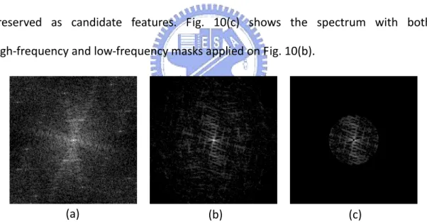
2 1 2 2 ) , ( ) , ( ) , (u v R u v I u v F = + (14) After applying Fourier transform on the target image, we perform the Fourier transform on the Fourier spectrum again to get the enhanced Fourier Spectrum. The enhanced Fourier spectrum is more prominent than the original spectrum. It reinforces the peaks with the same periods and contributes to the same frequency while for those which are not periodic ones, they do not contribute to the same frequency [13].This phenomenon relatively enhances those peaks and eliminates the non‐periodic noises in an image. Fig. 10(a) shows the Fourier spectrum of the target image in Fig. 8(a). Fig. 10(b) is the Fourier spectrum image obtained by applying Fourier transform on Fig. 10(a).
Low frequencies correspond to the slowly varying components of an image. For prints, these low‐frequency components are of enormous spectrum value and might result in noisy information. To remove these needless components, a mask for removing low‐frequency elements is applied. By masking, only frequencies that have Euclidean distance from the zero spatial‐frequency point greater than the predefined threshold are preserved as candidate features.
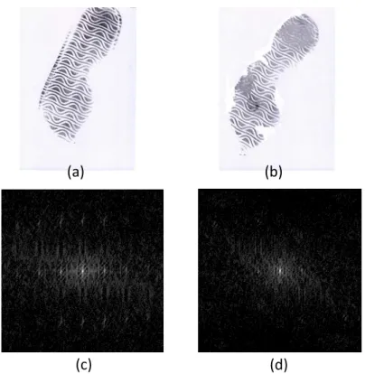
High‐frequency components which occur owing to outsole scuffs and nicks of the shoe may result in outstanding values over the underlying shoeprint patter [7]. Fig. 11 represents these high frequency noises. Similarly, a mask for removing the high‐frequency components is applied. Only frequencies that have Euclidean distance less than a predetermined threshold from the zero spatial‐frequency point are preserved as candidate features. Fig. 10(c) shows the spectrum with both high‐frequency and low‐frequency masks applied on Fig. 10(b).
Fig. 10. An example of the enhanced Fourier spectrum and the masking operation. (a) The Fourier spectrum of Fig. 8(a). (b) The enhanced Fourier spectrum of (a). (c) The spectrum with low‐frequency and high‐frequency masks apply on (b)
(a) (b) (c)
Following the procedure, the enhanced Fourier spectrum image that goes through low‐frequency and high‐frequency masks is denoted by F’ of size . Base on F’, we define a feature vector n n× , 1 , 1 | ) , ( ' {F i j i n j n GF = ≤ ≤ ≤ ≤ ( ji, ) is
Fig. 11. An example of the high‐frequency components. (a) A print with full integrity. (b) The same print with (a) with scuffs and nicks. (c) The enhanced Fourier spectrum of (a). (d) The enhanced Fourier spectrum of (b). (c) (d) (b) (a) 3.2.4 Local Fourier Transform
All three methods mentioned above take the full prints into consideration. Nevertheless, features extracted merely from the full image might lose details in local areas. To compensate this shortage, the local Fourier Transform based on the frequency domain is used. The processed shoeprint image is divided into 15 equal regions as shown in Fig. 12(a). Following that, Fourier transform is performed on each region twice to get the enhanced Fourier spectrum of the area. Low‐frequency mask and High‐frequency mask are also applied on each region k to get the masked Fourier spectrum . The remaining values, which are denoted by k F ' ) , ( 3 / ,..., 1 5 / ,..., 1 15 ,..., 1 | ) , ( ' {F i j k i n j m i j LF = k = = = is neither in
Fig. 12(b) shows a result after applying local Fourier transform on Fig. 12(a).
Fig. 12. An example of local Fourier transform. (a) A representation of dividing an image into 15 equal regions. (b) The result of applying local Fourier transform of Fig. 8(a) (a) (b)
3.3 Pattern Matching
Feature vectors extracted from the operations described above, including CM,
DM, GF, and LF, are taken for pattern matching at this stage.
In order to obtain the most likely shoeprint image that compares to the reference image, we use sum‐of‐absolute‐difference (SAD) as the similarity measure. The SAD is the most primitive technique for matching. Let images T and T" be the database image and reference image respectively, the similarity between the selected feature vector of the image pair is calculated by
∑
= − = K i i i F F K F S 1 " 1 ) (where denotes the element of a feature vector , and . i F th i F } , , , {CM DM GF LF
F∈ K denotes for the number of elements in the feature vector. F is a feature vector belongs to T . is a feature vector belongs to
'
F
'
from the database is corresponding to the examined shoeprint. Prints of databases are then sorted according to the similarity measure with the most similar image shown at the front of the results. Scores are given to the sorted categories of database from 1 to 315.
Combination of multiple feature vectors is conducted by summing up the given scores of each category from every individual feature vector. The lower the sum of the score means the more similar the category is comparing to the reference image. Therefore, categories are sorted according to the total scores by increasing order.
3.4 K‐means Algorithm for Database Creation
K‐means algorithm is a common algorithm for clustering. More specifically, it is an algorithm to group the objects based on attributes into K number of groups. Hence, for each of the print sets of 10 shoeprint images, we use the K‐means algorithm to select 3 representative images as the database category.
Feature vectors CM , DM , GF , and LF extracted using the methods described above are taken as attributes f ={CM,DM,GF,LF}, and used in the K‐means algorithm to form three groups. The algorithm performs the following steps until convergence: 1. Determine the centroid coordinate of each group. In the first iteration, shoeprints are assigned randomly into 3 groups. 2. Determine the distance of each shoeprint to the centroid of each group. The distance is calculated by Euclidean distance
∑
= − = K i i i c f dist 1 2 ) (Where denotes the attribute of the shoeprint image, and denotes the attribute of the centroid.
i
f ith ci
th
3. Group the shoeprints based on the minimum distance.
Each shoeprint is assigned to the group with the minimum distance. If no new assignment is performed, then the grouping procedure ends. Otherwise, repeat step 1 to step 3.
After applying the K‐means algorithm, we will have three groups of images for each individual shoeprint image set. From each group, the image with the closest disatance to the centroid of the group is taken as the representative image. The selected three images are then taken as database images. Seven of others are taken as query images.
Chapter 4
Experimental Results
Experiments are conducted to evaluate the performance of the proposed method. 1050 shoeprint images collected from 105 distinct shoes a re used to test our algorithm. 315 out of 1050 prints are taken as the database images according to the K‐means process described above. The remaining 735 shoeprint images become the query images. Fig. 13 shows 105 distinct shoeprints. Every print in the database is examined in turn for comparison with the input shoeprint. The similarity measures calculated based on each feature vector are then used to sort the shoeprint images in the database from the most similar print to the least similar one.
The method is designed to find similar shoeprints and sort the corresponding categories of database in response to a reference image. With higher performance, the result is expected to present fewer nonmatching shoeprint categories before a matching category. In view of this, “Average Match Score (AMS)“ is used to evaluate the performance of the results.
The “Average Match Score” measures the average percentage of the database categories before a correct match is delivered. In our experiments, each shoe pattern contains 3 corresponding shoeprint images in the database which are gathered from an identical right shoe. Hence, the performance is determined by counting the number of nonmatching categories until hitting the correct one. Then, the process continues to find the second and the third category that correctly matches to the reference shoeprint image with their searching cost.
Table 2 displays an example of query. With respect to the query shoeprint, each row shows the top 5 query results according to different feature vectors. In the first row, taking the feature vector of co‐occurrence matrix, the correct matching is
delivered in the 3rd, the 4th, and the 5th position. While taking all features into consideration, the correct matching is delivered in the 1st, the 2nd, and the 4th position. ‐ Query Results 1st 2nd 3rd 4th 5th Co‐occurrence Direction Global Fourier Local Fourier Query shoeprin t All TABLE 2 An Example of Query Results
Each feature vector is conducted independently first, and then combined together for further assessment. The best performance is the one with the combination of all proposed features vectors. Table 3 shows the results of AMS of the method in [7], which utilizes Fourier transform for matching. From the first column of
images should be examined in average to get one correct match. While for getting all three matching shoeprints, 13.88% of shoeprint database images should be examined in average. Results of the proposed method for different feature vectors are shown in Table 4. From the table we can see that 1.29%, 4.71%, and 11.59% of shoeprint database images should be examined in average respectively before the 1st, the 2nd, and the 3rd correct matching with the feature vector of co‐occurrence matrix. While taking all features into consideration, 0.38%, 1.19%, and 2.75% of the database images are examined in average before retrieving the 1st, the 2nd, and the 3rd correct shoeprint. The proposed method is much more accurate than the method provided in [7].
First Data Second Data Third Data Average
AMS (%) 3.51 11.75 26.39 13.88 TABLE 3 Average Match Scores (%) for the Chazal and Flynn’s Method on the Proposed Shoeprint Images with Image Resolution of 512x512
Features
First Data Second Data Third Data AverageCo‐occurrence 1.29 4.71 11.59 5.86 Direction 1.61 5.68 13.71 7 Global Fourier 0.64 3.09 7.39 3.71 Local Fourier 0.92 3.03 7.67 3.87 All Features 0.38 1.19 2.75 1.44 TABLE 4 Average Match Scores (%) for the Proposed Method on 735 Shoeprint Images from 105 Individual Shoes, Database of 315 Shoeprint Images with Different Features
Chapter 5
Conclusion
The study proposed a novel method for automatically recognizing the shoeprint image using the properties of directionality. Firstly, a series of preprocessing processes are applied to eliminate distortions in the print including rotations, translations, and noises. Four feature extraction methods based on the directionality are then performed on the preprocessed image. In the end, a similarity measure using SAD is calculated in response to the reference image.
Based on the algorithm, a system can be built to help forensic scientists seeking for the model of a shoe from a shoeprint image. Experiments designed for assessment of performance showed the accuracy and efficiency of the proposed method. It can accelerate human observer identifying the shoeprint pattern with respect to the reference image. However, shoeprints used in the study were obtained under human controlled circumstances, while those acquired at crime scene were of lower quality and of desperate distortions. These shoeprints were mostly partial prints and tough for matching. Improvements may be achieved by employing new de‐noise methods in preprocessing and delicately designed the database images from acquired shoeprints.
References
[1] A. Girod, “Computer Classification of the Shoeprint of Burglar Soles,” Forensic Science Int’l, vol. 82, pp. 59‐65, 1996.
[2] A. Girod, “Shoeprints ‐ Coherent Exploitation and Management,” European Meeting for Shoeprint/Toolmark Examiners, The Netherlands, 1997.
[3] W.J. Bodziak, “Footwear Impression Evidence Detection,” Recovery and Examination, 2nd ed. CRC Press, 2000.
[4] N. Sawyer, “’SHOE‐FIT’ A Computerized Shoe Print Database,” Proc. European Convention on Security and Detection, pp. 86‐89, May 1995.
[5] W. Ashley, “What Shoe Was That? The Use of Computerized Image Database to Assist in Identification,” Forensic Science Int’l, vol. 82, pp. 67‐79, 1996.
[6] A. Bouridance, A. Alexander, M. Nibouche, and D. Crookes, “Application of Fractals to the Detection and Classification of Shoeprints,” Proc. 2000 Int’l Conf. Image Processing, vol. 1, pp. 474‐477, 2000.
[7] P. de Chazal, J. Flynn, and R. B. Reilly, “Automated Processing of Shoeprint Images Based on the Fourier Tranform for Use in Forensic Science,” IEEE Trans. Pattern Analysis and Machine Intelligence, vol. 27, no. 3, pp. 341‐350, March 2005.
[8] K. Jack, “Video Demystified,” 5th ed. Elsevier, 2007
[9] R. Fisher, S. Perkins, A. Walker, and E. Wolfart. “Image Processing Learning Resources,” http://homepages.inf.ed.ac.uk/rbf/HIPR2/gsmooth.htm. [10] R. C. Gonzalez, R. E. Woods, “Digital Image Processing,” 2nd ed. Addison Wesley, 2002. [11] R. M. Haralick, “Statistical and Structural Approach to Texture,” Proc. IEEE, vol. 67, no. 5, pp. 786‐804, 1979. [12] A. K. Julesz, “Dialogues on Perception,” MIT Press, Cambridge MA, 1995.
[13] K. L. Lee, L. H. Chen, “A New Method for Coarse Classification of Textures and Class Weight Estimation for Texture Retrieval,” Pattern Recognition and Image Analysis, vol. 12, no. 4, pp. 400‐410, 2002.