pp. 25-46
現貨市場之投資人群聚行為與情緒變
數對台灣股價指數期貨之影響
The Effect of Herding Behavior and the Sentiments of
Investors on Taiwan Stock Index Futures
張巧宜1
Chiao-Yi Chang
國立臺中科技大學 保險金融管理系
Department of Insurance and Finance, National Taichung University of Science and Technology
陳香蘭 Hsiang-Lan Chen
國立高雄第一科技大學 財務管理系
Department of Finance, National Kaohsiung First University of Science and Technology
楊馥嫣 Fu-Yen Yang
國立高雄第一科技大學 金融系
Department of Money and Banking, National Kaohsiung First University of Science and Technology 摘要:過去研究忽略期貨市場受到情緒變數與現貨市場之群眾行為之影響, 本研究分析台灣指數期貨之報酬率如何受到 14 個金融市場之情緒變數的影 響,這些變數涵蓋現貨、期貨、與選擇權市場的變數,進而探討是否在期貨 價格上漲或下跌時研究結果皆相似。首先,我們以橫斷面之絕對離散度 (CSAD)模型、與狀態空間模型衡量台灣現貨市場的群聚現象,實證結果顯示, 台灣現貨市場存在群眾行為。另外,實證結果發現,當現貨市場群聚程度較 小時,指數期貨報酬降低,而當現貨市場群聚程度較大時,指數期貨之報酬 增加。特別值得注意的是,在期貨報酬大幅下降期間,當現貨市場之群聚程 度縮小,期貨報酬降低。此結果反映了在價格下降時,有較大的不確定性。 而為考慮在期貨價格上漲或下跌期間,不同程度的群聚行為與其他的解釋變 數的關聯性,呈現不同的結果,我們分別在正向、與負向之期貨報酬下,重 新衡量前述的模型,而實證結果仍然是被支持的。 關鍵詞:群聚行為;橫斷面之絕對離散度;投資人情緒變數;狀態空間模型
Abstract:This paper addresses the impacts of sentiment variables and herding
behavior on spot markets within the context of Taiwan Stock Index Futures. We
1 Corresponding author: Department of Insurance and Finance, National Taichung University of Science and Technology, Taichung City, Taiwan, E-mail: [email protected]
examine the variance in the rates of return of the Taiwan index futures based on 14 sentiment variables. These 14 variables include the sentiment variables in the spot, futures, and options markets. This paper further examines whether the results are consistent during bear and bull market periods. This study uses the cross-sectional absolute deviation (CSAD) model and the state space model to measure the herding behavior phenomenon in the spot market in Taiwan. Our results reveal that herding behavior is present in the Taiwan stock market, with empirical results showing that the index returns on futures fall when herding behavior mitigates in the stock market and rise when herding behavior is prevalent in the stock market. Notably, sharp decreases in futures returns are associated with decreased herding behavior and lower futures returns. This finding may reflect a higher degree of uncertainty during downward price movements. The present study finds consistency in analysis results during both bull and bear market periods.
Keywords : Herding behavior; Cross-sectional absolute deviation; Investor
sentiments; State space model
1.Introduction
Herding behavior, a phenomenon within behavioral economics, refers to the tendency of individuals to align their personal perspectives, judgments, and behavior with those of the group. Numerous studies have explored the impact of sentiments and of herding behavior in the stock market. However, studies of the futures market, particularly compared the spot market, have paid minimal attention to the impact of sentiment variables and herding behavior. This problem has left unclear an important factor that is generally acknowledged to affect futures-market operations.
This article examines the effects of 14 sentiment variables on the rates of return of Taiwan index futures. The findings are intended to give investors a better understanding of the impact of the herding behavior effect on other sentiment variables so that these variables may be taken into consideration when investing in Taiwan index futures. Additionally, the robustness of the results are examined under conditions of large movements both upward and downward in futures-market prices. Overall, this assessment of the impact of variables related to investor sentiments provides to futures investors a more comprehensive picture of market conditions.
The cost-of-carry theory defines the futures price as equal to the current spot price plus the carrying cost. Therefore, spot returns significantly influence futures returns. This article focuses on the issue of herding behavior in the context of the spot market. The herding behavior effect on the spot market has been studied previously. In the cross-sectional standard dispersion (CSSD) model,
dummy variables were used to simulate various market conditions and to reveal the effects of herding behavior on individual asset returns in the US equity market (Christie and Huang, 1995). The CSSD model suggests that if herding behavior exists during periods of large price movements then the individual stock returns should not diverge from the overall market return. Chang, Cheng and Khorana (2000) subsequently created the cross-sectional absolute deviation (CSAD) model that, as a variant of the CSSD model, also explains herding behavior. The CSAD model uses changes in actual market returns in place of the dummy variables specified in the CSSD model in order to account for non-linear relationships. The model suggests that if herding behavior exists during periods of large price movements, then the standard cross-sectional dispersion increases in proportion to the overall market return. This study employs the CSAD model to measure the level of herding behavior in a spot market2 and the associated effect of this behavior on futures returns.
State space is another model addressed in this paper by drawing on and Hwang and Salmon (2004)’s models as the basis for examining herding behavior in spot markets. In summary, this study has three research objectives this study has three research objectives. First, this study measures the extent of the herding behavior phenomenon in the spot market in Taiwan using regression and state space models. Second, this study evaluates the effects on futures returns of herding behavior and sentiment variables. Third, this study explores whether large upward/downward price swings in the futures market affect the abovementioned relationships.
The Taiwan Stock Exchange (TSE) provides a good example of an index futures market in a newly developed economy. We study this market using 14 sentiment variables. These variables are categorized into three sources: the spot market, the futures market, and the options market. The herding indicator facilitates the exploration of the effects of investor sentiments on futures returns. Additionally, this study considers the extent of herding behavior in the spot market to elicit the impact of large price movements in the futures market. The empirical results demonstrate that the positive relationship between level of herding behavior in the spot market and futures returns during sharp decreases in futures returns.
2.Literature Review
2
Since the herding behavior model is based on stock market, herding behavior has not, yet, been identified in futures markets. This might because there is the only one kind of underlying asset (stock index) in stock index futures; while herding behavior is discussed in the context of aligning investors among “many individual investment targets (individual firms)”.
The herding behavior effect is an irrational behavior that is often triggered by uncertainty. Herding behavior influences the investment behavior of individuals, ultimately resulting in the imitation or blind following of the decisions of others and the abandonment of preexisting information and decisions (Bikhchandani and Sharma, 2000). Nofsinger and Sias (1999) defined herding behavior as the tendency of investors to flock in the same direction at a specific time. Christie and Huang (1995), using the CSSD regression model, found no empirical evidence of herding behavior in the U.S. NYSE or AMEX. Chang, Cheng and Khorana (2000) modified the CSSD regression model and capital asset pricing model (CAPM) to create the CSAD model as a means of exploring herding behavior in developed economies including the U.S., Hong Kong, and Japan and in developing economies including South Korea and Taiwan.
Some studies have confirmed the influence of herding behavior in, such as Asia (Chiang and Zheng, 2010) and Greece (Caporale, Economou and Philippas, 2008). However, studies of the financial market in China have produced inconsistent empirical results. While Tan et al. (2008) found herding behavior as a factor of influence in the trading of A- and B- shares, Fu and Lin (2010) did not3. In sum, current evidence as assessed using the CSAD model supports that stock markets in developing economies tend to exhibit herding behavior and that this behavior has a less significant impact in developed economies. Beyond the CSAD model, Hwang and Salmon (2004) used the state space model to detect herding behavior in both the U.S. and South Korea. Their work provides another non-linear model besides CSAD to estimate herding behavior.
Chang, Cheng and Khorana (2000) found that herding behavior is more visible in upward than downward movements in the market. The degree of cross-section dispersion increased with the decay rate during periods of large market movement in developing countries such as Taiwan and South Korea, where a significant herding phenomenon exists. Their finding that herding behavior is largely absent in developed countries aligns with the findings of other studies (e.g., Christie and Huang, 1995). Chiang and Zheng (2010) found significant herding behavior in the two sub-markets of the U.S. and Latin America. Fu and Lin (2010) found that stocks affected by low turnover in the China market were affected by high levels of herding behavior during downward movements in the market. Gleason, Mathur and Peterson (2004) evaluated herding behavior in the Exchange Trade Fund (ETF) of the S&P Index under large price movement conditions, with empirical results showing no significant herding behavior in the ETF when the market exhibited extreme returns. Chang et al. (2012) reported that pronounced herding tendency of investor sentiments and trading for great events
3 Tan et al. (2008) used data from July 1997 to December 2003. Fu and Lin (2010) used data from January 2004 to June 2009, a period marked by a financial panic.
in Taiwan. Lin and Ma (2014) mentioned the herding for individual investors in Taiwan changes depending on market transparency. Therefore, the herding behavior in Taiwan exists and it may influence the return of stock market.
Psychological factors and sentiments not related to herding behavior also help shape the decisions of investors. These variables must be considered as well to fully understand investor decisions. Brown and Cliff (2004) distinguish between direct and indirect sentiment variables. Direct sentiment variables are assessed through interviews or collected by scales such as the Investors Intelligence Sentiment Indicator and the American Association of Individual Investor (AAII) Sentiment Indicator. Indirect sentiment variables are measured using real-market trading data such as the interbank overnight interest rate, the difference between the buy and sell volumes of institutional investors, put/call ratios, and the volatility index (VIX).
Many studies have explored the relationship between indirect sentiments and asset returns. Baker and Wurgler (2007) found that the link between indirect investor sentiments and investors’ sentiments is helpful in predicting stock returns. This suggests that investor sentiment readily affects those stocks that are relatively more difficult to evaluate. Yu and Yuan (2011) postulated that investor sentiment affects return-volatility tradeoff, especially in pessimistic periods. Kuhnen and Knutson (2011) report the effect of sentiment on financial decisions. As shown by Stambaugh, Yu and Yuan (2012), investor sentiment plays a negative predictor for the short legs of long-short investment strategies. Baker, Wurgler and Yuan (2012) found prediction power of investors sentiments among international markets. Because the preponderance of the literature to date has investigated the effect of sentiments on stock returns, there remains a lack of scholarly understanding of the impact of sentiments on futures returns.
The present study draws on measures of sentiment that were identified as significant in the literature. We outline the indicators and the reasons for choosing each of the measures in the following sections. First, we included sentiment indicators that relate to trading activity. Short-term lending rate percentages (i.e., the overnight interest rate) represent investor sentiment and share an inverse relationship with stock returns (Brown and Cliff, 2004). Second, we incorporated indicators of stock market trading activity (Brown and Cliff, 2004) such as the ratio of purchase-on-margin borrowing. We also adopted measures of trading activity from both the futures and options market because these measures relate to all three types of financial markets due to the sharing among these markets of the same underlying assets.
Additionally, the present study includes measures of open interest or the total unilateral power of pending statements in futures markets. The amount of open interest represents the potential market momentum and the total number of open interests represents the strength of short selling deadlocks and the degree of
price fluctuations. Bessembinder and Seguin (1993)’s study of eight types of futures contracts found a significant and negative relationship between the expected prices of open interest and futures. The present study considers a range of variables aside from open interest that relate to trading activity in the futures market, including: trading volume, initial margin, the institutional investor short-sale ratio, and the difference between buy and sell volumes for individuals and institutional investors in the futures market.
The present study uses the spot price minus the futures price, called the “basis”, to measure market performance. Hsu and Wang (2004) argue that rising expectations for futures market prices reflect a continuing contango and the opposite reflects a backwardation in that these expectations are heavily influenced by investor expectations with regard to stock prices. Both Inci and Lu (2007) and Gospodinov and Jamali (2011) confirmed the relationship between the return basis and futures returns. Investors frequently use the basis measure to help forecast futures returns in the real world.
Finally, the trading activity related to options is also an important indicator of investor sentiments. This study incorporates the frequently used VIX sentiment variable. Whaley (2000) highlights that VIX may broadly represent an index of investor expectations in the futures market or specifically represent a fear gauge for the securities market. A high value for VIX reflects pessimistic investor expectations and anticipates high market volatility. Simon and Wiggins (2001) also found the put/call ratio to be an important predictor of futures prices. In sum, all of the abovementioned factors were adopted and used in the present study to assess the effect of the financial-market-related sentiments of investors on futures returns.
3.Methodology
We combined the data on futures contracts with different expirations under the consideration of the maturity effect to obtain continuous data in the futures market. To avoid abnormal fluctuations in the data, we used data from the most recent month of index futures in Taiwan. This study employed a regression model to evaluate the relationship between sentiment indicators using herding measurement and futures returns. This study examined 14 investor sentiment variables across three financial markets (i.e., spot, futures and options market).
Data collected in the spot market included: the interbank overnight interest rates (IR), the ratio of purchase on margin (MR), the ratio of short sale (SC), and the herding behavior indicator (HERD). Data collected in the futures market included: basis (BS), open interest (OI), trading volume (VOL), initial margin (MAR), institutional investor short sale ratio (TH_RATIO), difference between the buy and sell volumes of individual investors (FUT ), and the difference between a
the buy and sell volumes of institutional investors (FUT ). Data collected in the p
options market included: the put/call ratio (P_C), the difference between the buy and sell volumes of individual investors in the options market (OPT ), the a
difference between buy and sell volumes of institutional investors (OPT ), and p VIX. Table 1 shows the sentiment variables related to each market. Additionally,
we added lag spot returns to explain futures returns because this variable is an important proxy of economic conditions4.
Following the example of Chang, Cheng and Khorana (2000), the present study used the CSAD variables to formulate a non-linear model to investigate the herding behavior effect, as follows:
t t m t m t c R R CSAD 1 , 2 2, (1) t up t m up t m up up t c R R CSAD 1 , 2( ,)2 (2) t down t m down t m down down t c R R CSAD 1 , 2( , )2 (3) with CSADt
Ni1Ri,t Rm,t /N, the absolute mean deviation of the return on
each stock i on day t and Ri,t indicating the market return Rm,t on day t.
N i it t m R N R 1 ,, / , represents the stock-market return on day t
5
, with N equal to the total number of stocks. Rmup,t (Rmdown,t ), and up
t
CSAD ( down
t
CSAD ) represent dispersion indicators in the bull (bear) market. We recalculated the CASD using capitalization weights to confirm the signs of coefficients in order to improve the robustness of the results. The CAPM model assumes that market investors are rational in order that the securities returns form a linear relationship with market beta risk in and that the market returns forms a linear relationship with the cross-sectional dispersion of the security returns. If herding behavior exists, then the relationship between the cross-sectional dispersion and the market return should be non-linear. Under this scenario, the market return and dispersion indicator do not increase proportionally or the correlation between the variables may weaken (when the coefficient 2 is negative).
4 When we experimented with adding current spot returns as an independent variable, the signs of the coefficients of the14 sentiment variables remained the same.
5
Due to the difficulties involved in categorizing the contributions to the stock market by investor type (e.g., overseas investors, securities dealers, mutual funds), the model does not make this distinction. Thus if the market is Rm = 3% on one day, the percentage of market return made on that day by different types of investors is unclear.
Table 1
Definitions of the Sentiment Variables
Panel A Definitions of the Sentiment Variables Variable
Category Variable Name
Variable
Symbol Variable Description
Dependent Variable
TAIEX index futures return
FR (Settlement price of TAIEX index futures on day t - settlement price on day t-1) / (settlement price on day t-1) Explanatory
Variable
Return of TAIEX RM Daily return of TAIEX from TEJ database Sentiment Indicators in Spot Market Interbank overnight interest rates
IR Interbank overnight interest rates in Taiwan Ratio of purchase on
margin
MR (Purchase on margin - Redemption) / (trading volume of Taiwan stock market 2) Ratio of short sale SC (Short Sale - Redemption) / (trading volume
of Taiwan stock market 2) Herding HERD
The coefficient 2 of rolling regression of equation (1)
Sentiment Indicators in Futures Market
Basis BS The daily price of Taiwan stock index – price of TAIEX index futures
Open interest OI Open interest of TAIEX index futures Trading volume VOL Trading volume of TAIEX index futures Initial margin MAR Initial margin of TAIEX index futures Institutional investor
short sale ratio
TH_RATIO Short volume of TAIEX index futures of the major institutional investors including dealers, investment trust companies, and foreign institutional investors/ (trading volume of TAIEX index futures 2)
Difference between buy and sell volume of individual investors in futures market
a
FUT Long volume of TAIEX index futures of
individual investors – short volume of TAIEX index futures of individual investors
Difference between buy and sell volume of institutional investors in futures market
p
FUT Long volume of TAIEX index futures of
institutional investors – short volume of TAIEX index futures of institutional investors
Sentiment Indicators in Options Market
Put/call ratio P_C Trading volume of put options/ trading volume of call options
Difference between buy and sell volume of individual investors in options market
a
OPT Long volume of Taiwan stock index options of
individual investors – short volume of TAIEX stock index options of individual investors
Difference between buy and sell volume of institutional investors in options market
p
OPT Long volume of Taiwan stock index options of
institutional investors – short volume of TAIEX stock index options of institutional investors
Volatility index VIX Volatility index on Taiwan stock index options
Panel B Definitions of the Dummy Variables
Explanatory Variable
Dummy Variable
Dummy variable of large falling market
TD_dn TD_dn = 1 for return of TAIEX index futures
falling exceed 2% TD_dn = 0 for other Dummy variable
of large raising market
TD_up TD_up = 1 for return of TAIEX index futures
We investigated the herding phenomenon in the stock market in Taiwan and then assessed its effect on futures returns. The 2 (i.e., “HERD”) is a measure of herding behavior, with higher negative values associated with an increased prevalence of herding behavior (Chang, Cheng and Khorana, 2000). A rolling regression model was then used to observe dynamic herding behavior (i.e.,2) in the spot market based on a 60-day window. The coefficient, 2 used to represent herding behavior in the spot market, was then added into the regression model as an independent variable.
Next, the present study employed the state space model with Kalman filter estimation (Demirer, Kutan and Chen, 2010) to enable a more thorough exploration of herding behavior, as follows:
mt mt imt H Std( )]1 log[ (4) mt mt mt H H 2 1 (5) where Hmt log(1hmt) , ~ (0, 2)
mt iid , and mt ~iid(0,2) , imt is the
market’s beta at time t. h is a time-varying latent herding behavior parameter. mt
When 0hmt 1 or 0, some degree of herding behavior exists in the market. There is no herding behavior when = 0 and Hmt = 0 for all t. Both
the regression model and state space model were used in this study, with consistent results on stock-market herding behavior between the two enhancing the rigor of findings.
We created a five-part categorization of the empirical models. Parts one to three addressed sentiment indicators that are exclusive, respectively, to the spot, futures, and options markets. Part four addressed sentiment indicators that relate to both the spot and futures markets. Part five addressed sentiment indicators that relate to all three markets. These models provide a basis to explore the connections between the trading activities and behavior of investors in each market and the returns earned on futures. Once herding behavior had been confirmed, the regression model was used to examine the results. This step integrated all of the sentiment variables from the spot, futures, and options markets as explanatory variables:
FRt = β0 + β1IRt + β2MRt + β3SCt + β4HERDt + β5BSt + β6OIt
+ β7VOLt + β8MARt + β9TH_RATIOt + β10
a t FUT + β11 p t FUT + β12P_Ct + β13OPT + βta 14 p t OPT + β15VIXt+εt (6)
where βj is the coefficient to estimate the value of j between 0~15, εt is the error term, and εt ~ N(0, σ). In order to account for the potential impact of large price movements, extreme futures returns were included in the model with the addition
of dummy variables designed to explore the effect of large movements in futures returns. The TD_dn dummy variable is equal to one if the returns in the index futures in Taiwan falls more than 2% and zero if not. The TD_up dummy variable is equal to one for returns if the rise exceeds 2% and zero if not6. The models that describe the impact of extreme returns are:
FRt = β0 + β1IRt + β2MRt + β3SCt + β4HERDt + θ1TD_dn HERDt
+ β5BSt + β6OI t + β7VOLt + β8MARt + β9TH_RATIOt + β10
a t FUT + β11FUT + βtp 12P_Ct + β13 a t
OPT + β14OPT + βtp 15VIXt+εt
(7)
FRt = β0 + β1IRt + β2MRt + β3SCt + β4HERDt + θ1TD_up HERDt
+ β5BSt + β6OIt + β7VOLt + β8MARt + β9TH_RATIOt + β10FUT ta
+ β11FUT + βtp 12P_Ct + β13OPT + βta 14OPT + βtp 15VIXt + εt
(8)
where βj is the coefficient used to estimate the value of j between 0~15, εt is the error term, and εt ~ N(0, σ). θ1 is the coefficient of the dummy variable. The term
TD_dn HERDt and TD_up HERDt are included to observe the relationship between the HERD and the futures returns under conditions when futures returns move sharply. Hence, for relatively large fluctuations in futures returns (2%), the coefficients for the HERD are β4 + θ1. For relatively small fluctuations in futures returns (2%), the coefficient is β4.
We added the lag spot returns, RMt-1, as an independent variable and reexamined equations (6), (7), and (8) in order to observe whether the coefficients associated with the sentiment variables had changed. This was done because the lag-stock returns are fairly good predictors of futures returns and because stock returns may be used as a proxy for the economy situation. Finally, to allow for the possibility that the level of herding behavior and other explanations may be asymmetric in the bear/bull futures market, we reexamined the model under two scenarios: positive futures returns and negative futures returns.
4.Data and Empirical Results
The data used in this study was drawn from the Taiwan Economic Journal (TEJ) Data Bank. The empirical test covers the period from July 21, 1998 (the day
6 The proportions of TD_dn and TD_up to all data are 10.25% and 10.94%, respectively. The two proportions are approximately the same and it is fair to use the two dummy variables to represent positive and negative extreme futures returns. The size is appropriate to observe the extreme returns (about 1/10) even we also used different thresholds of, say +/- 3%. The sample sizes of dummy variables that exceed 3% or -3% are 5.76% and 4.63%, respectively and the coefficients of the two dummy variables in the regression model are the same.
that index futures were inaugurated in Taiwan) to December 31, 2009 with a total of 2895 single-day data points. Because the institutional investor short sale ratio was made available only from July 2, 2007, the models related to this ratio cover only the period from July 2, 2007 to December 31, 2009. Additionally, because the VIX of options in Taiwan was made available only from December 1, 2006, the time frame of the models related to this variable was similarly shortened to match the available data. Table 2 reports the descriptive statistics for sentiment variables, spot returns, and futures returns. Over the sample period, the mean for futures returns was slightly positive (0.0244%), with a standard deviation of 1.87% and excess kurtosis.
4.1 Herding Behavior in the Spot Market
This study implemented the CSAD regression model and the state space model. To investigate herding behavior in the stock market. The results are shown in Table 3. The coefficients in Panel A, Table 3 reveal that a non-linear relationship exists between stock-market returns and cross-section dispersions of equity return due to the significant negative coefficient (-0.028) of the quadratics term in equation (1). The results support that the cross-sectional dispersion of return increases at a decreasing rate and then decreases after a specified peak as the stock returns become larger in absolute value. According to Chang, Cheng and Khorana (2000), the nonlinear relationship evidences the presence of herding behavior in the Taiwan stock market. The empirical results of this study are similar to Chang, Cheng and Khorana (2000), which suggested that the presence of large numbers of relatively short-term speculators as a cause of herding behavior in the TSE.
To allow the different coefficients under positive and negative returns, the two scenarios were examined and we included the same signs of the 2 coefficients in equation (2) and equation (3). Investors were found to exhibit significant herding behavior in cases of both positive and negative stock returns (-0.018, and -0.031, respectively). The larger negative coefficient 2 in the downward market indicates that herding behavior is stronger for negative stock returns than for positive stock returns. The results in Panel A for equally weighted CSAD and in Panel B for capitalization-weighted CSAD are similar in terms of signs.
4.2 The Connection between Herding Behavior in the Spot
Market and the Return on Futures
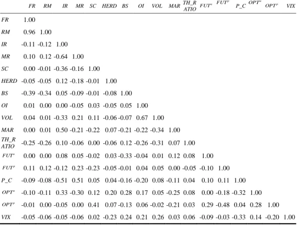
We checked the correlations of variables to avoid the problem of collinearity in the regression model as shown in Table 4. None of the absolute values of correlation was larger than 0.7. Therefore, no significant collinearity
Table 2
Descriptive Statistics of Sentiment Variables
FR is Taiwan index futures return. RM is Taiwan stock return. IR is interbank overnight interest
rates. MR is ratio of purchase on margin. SC is ratio of short sale. HERD is herding indicator. BS is basis. OI is open interest. VOL is trading volume. MAR is initial margin. TH_RATIO is institutional investor short sale ratio. a
FUT is the difference between buy and sell volume of
individual investors in futures market. p
FUT is the difference between buy and sell volume of
institutional investors in futures market. P_C is put/call ratio. a
OPT is the difference between
buy and sell volume of individual Investors in options market. p
OPT is the difference between
buy and sell volume of institutional investors in options market. VIX is volatility index.
Panel A Sentiment Variables in Spot Market
Variable Symbol FR RM IR MR SC HERD
Sample Period 1998/07/21 to 2009/12/31 Sample Size 2,985.00 2,985.00 2,985.00 2,985.00 2,985.00 2,895.00 Mean 0.02 0.01 2.39 26.13 2.15 1.94 Standard Deviation 1.87 1.62 1.66 8.53 1.30 0.43 Kurtosis 2.52 4.74 -0.63 -0.58 9.66 0.65 Skewness -0.01 -0.01 0.72 0.51 2.20 0.79 Minimum -7.00 -6.67 0.10 9.45 0.00 0.43 Maximum 6.99 6.74 7.07 50.26 12.72 3.98
Panel B Sentiment Variables in Futures Market
Variable Symbol BS OI VOL MAR TH_R
ATIO a FUT p FUT Sample Period 1998/07/21 to 2009/12/31 2007/07/02 to 2009/12/31 Sample Size 2,895.00 2,895.00 2,895.00 2,895.00 628.00 628.00 628.00 Mean 5.27 23,219.00 25,591.00 11,081.00 13.71 670.26 -1,162.99 Standard Deviation 58.96 18,566.00 28,900.00 25,495.00 3.44 15,692.90 5,735.81 Kurtosis 2.44 -0.76 2.91 0.02 5.21 0.48 2.81 Skewness -0.27 0.52 1.71 0.74 1.34 0.65 -1.43 Minimum -377.76 36.00 0.00 75,000.00 0.00 -23,631.00 -19,282.00 Maximum 332.87 83,020.00 172,208.00 195,000.00 38.13 44,512.00 8,521.00
Panel C Sentiment Variables in Options Market
Variable Symbol P_C OPTa OPTp VIX
Sample Period 2006/12/01 to 2009/12/31 Sample Size 767.00 767.00 767.00 767.00 Mean 0.87 -2,667.52 3,648.72 29.48 Standard Deviation 0.26 114,069.00 17,434.00 9.13 Kurtosis -0.25 -0.05 3.50 0.16 Skewness 0.22 0.20 0.54 0.46 Minimum 0.22 -238,850.00 -40,648.00 11.74 Maximum 1.80 285,642.00 61,356.00 60.41
Table 3
Empirical Non-Linear Relationships between Market Returns and Stock Dispersion Indicators Panel A and B show the regressions of the following forms are estimated using:
t t m t m t c R R CSAD 1 , 2 2, (1) t up t m up t m up up t c R R CSAD 1 , 2( ,)2 (2) t down t m down t m down down t c R R CSAD 1 , 2( , )2 (3) where CSADt R R /N N 1 i i,t m,t
, is the mean absolute deviation of the return of each stock i, Ri,t, relative to
the market return,
t m R ,. up t m R, ( down t m R , ) and up t
CSAD (CSADtdown) represent dispersion indicator on bull (bear)
market. The CSAD variable in Panel A is calculated by equally weighted base, while it in Panel B is calculated by market-value-weighted base. Panel C show the results of the following state space model:
mt mt imt H td( ))1 S log( (4) mt mt mt H H 2 1 (5) whereHmtlog(1hmt), ~ (0, ) 2 mt iid , and ~ (0, 2)
mt iid . When = 0, there is no herding and the Hmt= 0. When 0<hmt<1, the herding exists in the market.
Panel A Regression Model with Equally Weighted CSAD
Variable equation (1) equation (2) equation (3)
c 1.7350 *** 1.6769 *** 1.8310 *** (122.6305) (99.4797) (80.0290) 1 0.2394 *** 0.2023 *** 0.2296 *** (13.5467) (8.9287) (8.6136) 2 -0.0289*** -0.0188 *** -0.0314 *** (-7.4023) (-3.7328) (-5.4191) Adjusted R2 10.97% 12.10% 7.71%
Panel B Regression Model with Capitalization-Weighted CSAD
c 1.5305 *** 1.6747 *** 1.4308 *** (78.1901) (67.3070) (78.1902) 1 0.3163*** 0.2795 *** 0.2941 *** (16.3153) (9.6414) (11.8956) 2 -0.0491*** -0.0487 *** -0.0395 (-11.4484) (-7.7271) (-7.1859) Adjusted R2 10.84% 6.61% 13.38%
Panel C State Space Model 1 -0.7344*** (-22.0048) 2 0.8449*** (187.0759) 0.3095 (0.0042) 0.0275*** (4.7489)
Table 4 Correlation Matrix
FR is Taiwan index futures return. RM is Taiwan stock return. IR is interbank overnight interest
rates. MR is ratio of purchase on margin. SC is ratio of short sale. HERD is herding indicator. BS is basis. OI is open interest. VOL is trading volume. MAR is initial margin. TH_RATIO is institutional investor short sale ratio. a
FUT is the difference between buy and sell volume of
individual investors in futures market. p
FUT is the difference between buy and sell volume of
institutional investors in futures market. P_C is put/call ratio. a
OPT is the difference between
buy and sell volume of individual Investors in options market. p
OPT is the difference between
buy and sell volume of institutional investors in options market. VIX is volatility index.
FR RM IR MR SC HERD BS OI VOL MAR TH_R ATIO a FUT p FUT P_C a OPT p OPT VIX FR 1.00 RM 0.96 1.00 IR -0.11 -0.12 1.00 MR 0.10 0.12 -0.64 1.00 SC 0.00 -0.01 -0.36 -0.16 1.00 HERD -0.05 -0.05 0.12 -0.18 -0.01 1.00 BS -0.39 -0.34 0.05 -0.09 -0.01 -0.08 1.00 OI 0.01 0.00 0.00 -0.05 0.03 -0.05 0.05 1.00 VOL 0.04 0.01 -0.33 0.21 0.11 -0.06 -0.07 0.67 1.00 MAR 0.00 0.01 0.50 -0.21 -0.22 0.07 -0.21 -0.22 -0.34 1.00 TH_R ATIO -0.25 -0.26 0.10 -0.06 0.00 -0.06 0.12 -0.26 -0.31 0.07 1.00 a FUT 0.00 0.00 0.08 0.05 -0.02 0.03 -0.33 -0.04 0.01 0.12 0.08 1.00 p FUT 0.11 0.12 -0.12 0.23 -0.23 -0.05 -0.01 0.04 0.05 0.00 -0.05 -0.10 1.00 P_C -0.09 -0.08 -0.51 0.51 0.05 0.04 -0.16 -0.20 0.08 -0.11 0.04 0.10 0.11 1.00 a OPT -0.10 -0.11 0.33 -0.30 0.12 0.20 0.28 0.17 0.05 -0.25 0.08 0.00 -0.18 -0.32 1.00 p OPT -0.01 0.00 -0.05 0.00 0.41 0.07 -0.13 0.06 -0.02 -0.21 0.03 0.29 -0.48 0.04 0.28 1.00 VIX -0.05 -0.06 -0.05 -0.06 0.02 -0.23 0.24 0.21 0.26 0.03 0.06 -0.09 -0.03 -0.33 0.14 -0.20 1.00
problem was noted. After confirming the presence of herding behavior in the spot market, we adopted rolling regression models with a window size of 60 days in order to obtain a dynamic sequence of coefficients 2.The dynamic sequence of coefficients 2, called HERD, was re-estimated every 60 days. Equation (1) used 2836 (= 2895 – 60 + 1) regression-model calculations to find the continuous time varying herding behavior. Next, the series of coefficients 2 were incorporated with other sentiment variables in equation (6) of Table 5 to investigate the
relationship between return on futures and sentiment variables. Equations (7) and (8) in Table 5 were added TD_up HERD and TD_dn HERD, respectively.
The coefficients on the HERD are significantly negative in Table 5, with the exception of equation (7). The larger (less negative) HERD, the smaller the level of herding behavior in the spot market. Thus, the negative signs of coefficients of
HERD show the positive connection between the level of herding behavior in spot
market and the return on futures. The futures return index declines when herding behavior mitigates the stock market and the futures return index rises when herding behavior more seriously affects the stock market. Irrational herding behavior occurs in the spot market due to investors seeking potential gain from returns on futures. Herding behavior in the spot market exhibits a significant impact on future returns. This impact did not disappear after lag spot returns were added as a control variable, although we don’t show the results in the table.
As shown in Table 5, the coefficients of interbank overnight interest rates (IR) were significant negative, indicating that the sentiments of investors tend to be higher when the investing opportunity costs, such as IR, are lower. The negative coefficient of IR means that the returns on futures fall when investor sentiment is low. The basis (BS) has the expected negative sign, indicating that the low futures price coupled with low investors’ sentiment negatively affects futures returns. The coefficients of the futures trading volume (VOL) have negative signs in Table 5, regardless of whether spot returns or extreme future returns are added as an independent variable. This is unexpected, because the large trading volume often represents high sentiments. Therefore, investors should carefully judge the impacts of trading volume on futures returns.
Additionally, the short sales by the institutional investors (TH_RATIO) were found to have an inverse association with Taiwan stock futures returns. The positive coefficient of the difference between buy and sell of institutional investors (FUT ) suggests that Taiwan futures returns increased as the net p
number of futures purchases made by institutional investors increased. The low
TH_RATIO and high FUT represent high sentiment. Another unexpected sign p
is the negative coefficients of FUT . The low sentiments of individuals were a
accompanied by high futures returns. The possible reason for this phenomenon is that the individual represents only one type of market participant. The put/call ratio (P_C) has negative sign and OPT has a positive sign. Lower investor a
sentiments in the options market coupled with higher P_C and lower OPT a
were associated with higher futures returns.7
Equations (7) and (8) show the cross-term of herding behavior and large upward versus downward swings of futures returns. The effect of sharpfluctuations in futures returns on herding behavior is interesting to observe. The dummy variable TD_up sets to 1 if futures returns increase more than 2 % in equation (7), whereas the dummy variable TD_dn sets to 1 if futures returns decline by more than 2% in equation (8). In Table 5, the signs of the cross-terms in equation (7) are the opposite of those in equation (8). The coefficients of these cross-terms reveal that the effect of herding behavior is negative (-14.98) when futures returns fall more than 2%. When futures returns decrease sharply, the larger levels of herding behavior (smaller HERD or larger magnitude of negative
HERD) are concurrent with higher futures returns.
The coefficients of cross-term reveal that the effect of herding behavior is positive (15.23) when futures returns rise more than 2%. For the case in which futures returns rise sharply, the high level of herding behavior in spot market is accompanied by increasing futures returns. When futures returns do not decrease extremely, as in equations (7) and (8), the negative value of HERD means that the high level of herding behavior in spot market is accompanied by decreasing futures returns.
4.3 The Connection between Herding Behavior in the Spot
Market and Futures Returns during Bear and Bull Markets
Considering that herding behavior may affect positive/negative futures returns differently, we further divided the bear/bull futures market in Tables 6 to consider the different impacts of herding behavior. The second and third columns show tests of the effects of sentiment variables on negative futures returns (bear market), while the fourth and fifth columns show the effects of the same variables on positive futures returns (bull market). As stated earlier, larger (less negative) values for 2 are associated with smaller levels of herding behavior in the spot market. With regard to the case without cross-terms in Table 6, the coefficient of
HERD in equations (6) was not significant during the bull market. The negative
sign of HERD (-3.72) shows a positive connection between the level of herding behavior in the spot market and the futures returns during a bear market. The negative coefficients of HERD indicate that the futures returns, which do not
futures, and options market. In other words, only the intercept term, IR, MR, SC, and HERD variables are included in the regression model in the first round of estimation. For the second round of estimation, only the intercept, BS, OI, VOL, MAR, TH_RATIO, a
FUT , and p
FUT are included in the model. Finally, only the intercept, P_C, a
OPT , p
OPT , VIX variables are included in the third round. The signs are the same as the results of all 14 variables in the models.
decrease sharply during bear markets, tend to increase as with herding behavior in the spot market.
When futures returns increase sharply during a bull market, the empirical results are similar to those shown in Table 5.8 The coefficient of the cross-term remains negative (-15.61) when futures returns fall more than 2% during a bear market and turns positive (10.016) when futures returns rise more than 2% during a bull market. In Table 6, a positive value for TD_up HERD means that sharp increases in futures returns during a bull market is accompanied by decreased levels of herding behavior (larger 2 or small magnitude of negative 2) and higher futures returns. The negative coefficient of TD_dn HERD indicates that when futures returns decrease sharply during a bear market, the smaller level of herding behavior (larger 2 or small magnitude of negative 2) is accompanied by lower futures returns.
In summary, sharp rises in futures returns resulted in herding behavior in spot markets accompanied by decreasing futures returns. Sharp decreases in futures resulted in herding behavior in the spot market accompanied by increasing futures returns. Comparing other sentiment variables in Tables 6, we find that the signs of some variables such as IR, SC, MAR, and VIX are different during bear/ bull markets. That shows that investors hold different views of the same sentiment variable in the contexts of both positive and negative futures returns. For example, the VIXs are negative during the bear market and positive in the bull market. When market volatility increases during bear market conditions, investor panic related to market increased, reducing futures market returns. However, when market volatility increased during a bull market, investors may associate this increase with an opportunity to get more profits. Thus higher VIX values are associated with higher returns on futures.
Finally, sentiment variables including BS and P_C had the same signs regardless of whether the market was bull or bear. The two variables also represent the futures and options markets, respectively. The consistency in value of these variables in both bull and bear markets indicate that either investor sentiments affect futures returns or that a common factor ties these three financial markets together. Although forecasting the trend of futures returns in advance, the common variable through two scenarios identifies co-movement factors that are associated with futures returns.
8
It is not appropriate to add the TD_dn variable in markets with positive futures returns because the dummy variable TD_dn equals one in cases where the decline in futures returns exceeds 2% and zero for others. Thus, All data show that TD_dn equals zero for positive futures returns, which creates the problem of collinearity. Similarly, the dummy variable, TD_up is not appropriate for use in markets with negative futures returns.
Table 5
Estimation of the Regression Models for All Samples The regression of the following equation (6) is estimated using:
FRt = β0 + β1IRt + β2MRt + β3SCt + β4HERDt + β5BSt + β6OIt + β7VOLt + β8MARt + β9TH_RATIOt
+ β10FUTta + β11FUTtp + β12P_Ct + β13OPT + βta 14OPT + βtp 15VIXt + ε
(6) where FRt is the dependent variable representing the daily futures returns and the independent
variables can be found in Table 1. The equations (7) and (8) are added TD_dn HERD and
TD_up HERD, respectively.
Variable equation (6) equation (7) equation (8)
Intercept 5.3338 *** 5.0750 *** 5.1978 *** (4.6337) (4.4139) (4.5301) IR -0.5212 *** -0.5083 *** -0.4925 *** (-2.7967) (-2.7399) (-2.6492) MR 0.0366 0.0351 0.0401 (0.9871) (0.9496) (1.0842) SC -0.1449 -0.1538 -0.1337 (-0.7611) (-0.8116) (-0.7054) HERD -4.8451 ** -2.4997 -6.8597 *** (-2.0852) (-1.0084) (-2.8005) TD_dnHERD -14.9789 *** (-2.6253) TD_upHERD 15.2294 ** (2.5087) BS -0.0187 *** -0.0182 *** -0.0186 *** (-11.2961) (-10.9538) (-11.2959) OI -0.046210-5 -0.062410-5 -0.047210-5 (-0.0672) (-0.0912) (-0.0689) VOL -0.75110-5 ** -0.68610-5 ** -0.71410-5 ** (-2.1551) (-1.9716) (-2.0542) MAR 0.003310-5 0.02710-5 0.010810-5 (0.0087) (0.0729) (0.0293) TH_RATIO -0.1236 *** -0.1172*** -0.1220*** (-5.2002) (-4.9578) (-5.1810) a FUT -1.1610-5 ** -1.1810-5 ** -1.1410-5 ** (-2.1538) (-2.0431) (-2.1201) p FUT 2.9210-5 * 3.3410-5 ** 2.9410-5 * (1.8738) (2.1201) (1.8965) P_C -2.1982 *** -2.1169 *** -2.1563 *** (-5.4660) (-5.2742) (-5.3812) a OPT 0.20710-5 ** 0.20610-5 ** 0.20110-5 ** (2.1582) (2.1568) (2.1017) p OPT -0.27110-5 -0.16710-5 -0.22210-5 (-0.4658) (-0.2865) (-0.3828) VIX -0.0082 -0.0072 -0.0095 (-0.6346) (-0.5429) (-0.7400) Adjusted R2 26.88% 27.59% 27.52%
Note: ***, **, * denote statistical significances at the 1%, 5%, and 10% levels, respectively. The t-statistics calculated are in parentheses.
Table 6
Estimation of the Regression Models for the Bear and Bull Market The regression of the following equation (6) is estimated using:
FRt=β0+β1IRt+β2MRt+β3SCt+β4HERDt+β5BSt+β6OIt+β7VOLt+β8MARt+β9TH_RATIOt+β10FUTta
+β11FUTtp+β12P_Ct+β13OPT +βta 14OPT +βtp 15VIXt+ε
(6)
where FRt is the dependent variable representing the daily futures returns and the independent
variables can be found in Table 1. The equations (7) and (8) are added TD_dnHERD and
TD_upHERD, respectively.
Bear Market Bull Market
Variable equation (6) equation (7) equation (6) equation (8) Intercept 5.3822 *** 5.1182 *** -0.7418 -0.7573 (4.8754) (4.7343) (-0.6469) (-0.6648) IR -0.7661 *** -0.7530 *** 0.5850 *** 0.6100 *** (-4.1220) (-4.1457) (3.3646) (3.5244) MR -0.0394 -0.0503 0.1146 *** 0.1167 *** (-1.0253) (-1.3351) (3.3680) (3.4513) SC -0.3129 * -0.3528 * 0.4422 ** 0.4561 ** (-1.6818) (-1.9373) (2.3968) (2.4870) HERD -3.7171 * 0.8303 0.4560 -2.2666 (-1.6748) (0.3320) (0.2013) (-0.8916) TD_upHERD 10.0157 ** (2.3052) TD_dnHERD -15.6096 *** (-3.6512) BS -0.0106 *** -0.0096 *** -0.0062 *** -0.0063 *** (-5.9514) (-5.4228) (-3.8336) (-3.9243) OI 0.35210-5 0.29810-5 -1.0810-5* -1.0810-5 * (0.5030) (0.4359) (-1.6876) (-1.6970) VOL -0.58310-5 -0.45410-5 0.2910-5 0.3210-5 (-1.5776) (-1.2527) (0.9204) (1.0229) MAR 0.80610-5** 0.83310-5** -1.2110-5 *** -1.2110-5 *** (2.1199) (2.2440) (-3.6329) (-3.6577) TH_RATIO -0.1148 *** -0.1076 *** 0.0231 0.0214 (-5.0611) (-4.8333) (0.9524) (0.8895) a FUT -0.28610-5 -0.06810-5 -0.77810-5 -0.75510-5 (-0.5083) (-0.1227) (-1.6002) (-1.5620) p FUT 1.8610-5 2.610-5 * 0.48110-5 0.39410-5 (1.1935) (1.6916) (0.3287) (0.2711) P_C -1.2149 *** -1.0226 ** -1.5454 *** -1.5104 *** (-3.0157) (-2.5749) (-4.1303) (-4.0608) a OPT 0.08110-5 0.09410-5 -0.05810-5 -0.05810-5 (0.8038) (0.9637) (-0.6605) (-0.6753) p OPT -0.48810-5 -0.31610-5 -0.62110-5 -0.61510-5 (-0.8107) (-0.5351) (-1.1611) (-1.1566) VIX -0.0696 *** -0.0683 *** 0.0543 *** 0.0517 *** (-5.5801) (-5.6029) (4.4900) (4.3110) Adjusted R2 37.48% 40.31% 22.46% 23.46%
Note: ***, **, * denote statistical significances at the 1%, 5%, and 10% levels, respectively. The t-statistics calculated are in parentheses.
5.Conclusions
This study initially examined the connection between herding behavior in the Taiwan spot market and futures returns. After observing the relationship between equal-weighted/capitalization-weighted cross-section dispersion and stock returns, the empirical results of this study, obtained using the regression and state-space models, indicate that herding behavior exists in the spot market. After confirming that herding behavior exists in the Taiwan spot market, the dynamic herding behavior measure was included in the regression model as an investor sentiment variable in order to examine the association between sentiment variables and the Taiwan index futures returns. Considering 14 sentiment variables related to trading activity covering the spot, futures, and options markets, the empirical results support that herding behavior in the spot market has a significant impact on futures returns. This finding is one of the critical contributions of this study. Additionally, the empirical results showed that the index futures return is higher when the level of herding behavior in the stock market is higher and is lower when herding behavior mitigates the stock market. The empirical results are the same whether or not the spot returns are added to the models used to explain futures returns.
In terms of the large swings in futures returns, when futures returns decrease sharply, a low level of herding behavior accompanies lower futures returns. However, when the futures returns increase sharply, the herding behavior in the spot market is associated with decreasing futures returns. Furthermore, it is worth noting that an examination of the futures market shows that the coefficient of herding behavior is insignificant when the bull market and that the herding behavior effect of spot-to-futures returns is larger in bear markets than in bull markets. A partial explanation for the asymmetric effects of herding behavior between bull and bear markets is that the investors have a greater tendency to follow others blindly during bear markets owing the greater levels of uncertainty.
The authors hope that the administrative authority may reference the empirical results of this study when developing plans to improve the management of financial markets. The impact of herding behavior in the spot market suggests the importance of transparency and other market conditions to herding behavior in the stock market and, by extension, the futures market. Considering what factors lead to herding behavior in the spot market in order to develop strategies to minimize herding behavior is critical to decreasing volatility in futures markets. Caution is advised before applying the empirical results of this study to investing in terms of the actual connections among spot, futures, and options markets, which is another critical contribution of this study. Certain sentiment variables that are observed in different financial markets have a significant impact
on the futures market and should be considered among the comprehensive factors that affect financial markets when investing in futures.
References
Baker, M. and Wurgler, J. (2007), “Investor Sentiment in the Stock Market,”
Journal of Economic Perspectives, 21(2), 129-151.
Baker, M., Wurgler, J. and Yuan, Y. (2012), “Global, Local, and Contagious Investor Sentiment,” Journal of Financial Economics, 104(2), 272–287. Bessembinder, H. and Seguin, P. J. (1993), “Price Volatility, Trading Volume, and
Market Depth: Evidence from Futures Markets,” Journal of Financial and
Quantitative Analysis, 28(1), 21-39.
Bikhchandani, S. and Sharma, S. (2000), “Herd Behavior in Financial Markets: A Review,” IMF Staff Papers, 47(3), 279-310.
Brown, G. W. and Cliff, M. T. (2004), “Investor Sentiment and the Near-Term Stock Market,” Journal of Empirical Finance, 11(1), 1-27.
Caporale, G. M., Economou, F. and Philippas, N. (2008), “Herding Behaviour in Extreme Market Conditions: The Case of the Athens Stock Exchange,”
Economics Bulletin, 7(17), 1-13.
Chang, C. H., Tsai, C. C., Huang, I. H. and Huang, H. H. (2012), “Intraday Evidence on Relationships among Great Events, Herding Behavior, and Investors’ Sentiments,” Chiao Da Mangement Review, 32(1), 61-106.
Chang, E. C., Cheng, J. W. and Khorana, A. (2000), “An Examination of Herd Behavior in Equity Markets: An International Perspective,” Journal of
Banking and Finance, 24(10), 1651-1679.
Chiang, T. C. and Zheng, D. (2010), “An Empirical Analysis of Herd Behavior in Global Stock Markets,” Journal of Banking and Finance, 34(8), 1911-1921. Christie, W. and Huang, R. (1995), “Following the Pied Piper: Do Individual
Returns Herd around the Market?” Financial Analysts Journal, 51(4), 31-37. Demirer, R., Kutan, A. and Chen, D. (2010), “Do Investors Herd in Emerging
Stock Market? Evidence from the Taiwanese Market,” Journal of Economic
Behavior & Organization, 76(2), 283-295.
Fu, T. and Lin, M. (2010), “Herding in China Equity Market,” International
Journal of Economics and Finance, 2(2), 148-156.
Gleason, K. C., Mathur, I. and Peterson, M. A. (2004), “Analysis of Intraday Herding Behavior among the Sector ETFs,” Journal of Empirical Finance, 11(5), 681-694.
Gospodinov, N. and Jamali, I. (2011), “Risk Premiums and Predictive Ability of BAX Futures,” Journal of Futures Markets, 31(6), 534-561.
Hsu, H. and Wang, J. (2004), “Price Expectation and the Pricing of Stock Index Futures,” Review of Quantitative Finance and Accounting, 23(2), 167-184.
Hwang, S. and Salmon, M. (2004), “Market Stress and Herding,” Journal of
Empirical Finance, 11(4), 585-616.
Inci, A. C. and Lu, B. (2007), “Currency Futures-Spot Basis and Risk Premium,”
Journal of International Financial Markets, Institutions and Money, 17(2),
180-197.
Kuhnen, C. and Knutson, B. (2011), “The Influence of Affect on Beliefs, Preferences, and Financial Decisions,” Journal of Financial and
Quantitative Analysis, 46(3), 605-626.
Lin, Y. L. and Ma, T. (2014), “The Relationship between Pre-Trade Transparency, Order Imbalance and Investors’ Behavioral Biases,” Chiao Da Mangement
Review, 34(1), 79-116.
Nofsinger, J. R. and Sias, R. W. (1999), “Herding and Feedback Trading by Institutional and Individual Investors,” Journal of Finance, 54(6), 2263-2295.
Simon, D. P. and Wiggins, R. A. (2001), “S&P Futures and Contrary Sentiment Indicators,” Journal of Futures Market, 21(5), 447-462.
Stambaugh, R. F., Yu, J. and Yuan, Y. (2012), “The Short of It: Investor Sentiment and Anomalies,” Journal of Financial Economics, 104(2), 288-302.
Tan, L., Chiang, T. C., Mason, J. R. and Nelling, E. (2008), “Herding Behavior in Chinese Stock Markets: An Examination of A and B Shares,” Pacific-Basin
Finance Journal, 16(1), 61-77.
Whaley, R. E. (2000), “The Investor Fear Gauge,” Journal of Portfolio
Management, 26(3), 12-17.
Yu, J. and Yuan, Y. (2011). “Investor Sentiment and the Mean-Variance Relation,”