以LIBOR市場模型評價利率衍生性商品：結合二項樹方法

國

立 交 通 大 學

財 務 金 融 研 究 所

碩 士 論 文

以

LIBOR 市場模型評價利率衍生性商品：

結合二項樹方法

Using the LIBOR Market Model to Price

the Interest Rate Derivatives：

A Recombining Binomial Tree Methodology

研 究 生： 何俊儒

指導教授： 鍾惠民 博士

戴天時 博士

以

LIBOR 市場模型評價利率衍生性商品：

結合二項樹方法

Using the LIBOR Market Model to Price

the Interest Rate Derivatives：

A Recombining Binomial Tree Methodology

研 究 生：何俊儒

Student：Chun-Ju Ho

指導教授： 鍾惠民博士 Advisor：Dr. Huimin Chung

戴天時博士 Dr.

Tian-Shyr

Dai

國立交通大學

財務金融研究所

碩士論文

A Thesis Submitted to Graduate Institute of Finance

National Chiao Tung University

in partial Fulfillment of the Requirements

for the Degree of

Master of Science in

Finance

June 2008

Hsinchu, Taiwan, Republic of China

中華民國九十七年六月

以

LIBOR 市場模型評價利率衍生性商品：

結合二項樹方法

研究生：何俊儒 指導教授：鍾惠民 博士

戴天時 博士

國立交通大學財務金融研究所碩士班

2008 年 6 月

摘 要

本研究採用 Ho、Stapleton 和 Subrahmanyam 所提出的結合二項樹方法來建造 LIBOR 市場模型的遠期利率演進過程。此結合二項樹評價法對於評價利率衍生 性金融商品與之前所提出的利率模型相比，提供了我們一個計算方便且準確的數 值結果。此外在評價過程中，此結合二項樹評價法也比蒙地卡羅模擬法來的省時 且有效率。而用此結合二項樹評價法所計算出來的債券選擇權和利率上限買權價 值與理論值的誤差也在容忍的誤差範圍內。

關鍵字：結合二項樹評價法，LIBOR 市場模型，債券選擇權

利率上限選擇權

Using the LIBOR Market Model to Price

the Interest Rate Derivatives:

A Recombining Binomial Tree Methodology

Student: Chun-Ju Ho Advisors: Dr. Huimin Chung

Dr. Tian-Shyr Dai

Graduate Institute of Finance

National Chiao Tung University

June 2008

Abstract

In this thesis, we adapt the recombining node methodology proposed by Ho, Stapleton, and Subrahmanyam to implement the LIBOR market model (LMM). The lattice method we proposed is more efficient in comparison with Monte Carlo simulation as pricing the interest rate derivatives. The results of the bond option value and the caplet value are approximate to the theoretical value respectively.

致 謝

 

本篇的論文能夠順利的完成，首先要感謝鍾惠民老師與戴天時老師的細心指 導，竭盡心力的幫助學生在論文寫作中所遇到的困難與疑惑。感謝鍾惠民老師在 在繁忙的公務中，還要花時間幫學生搜尋資料與分析，提出對資料和分析的建議。 感謝戴天時老師無時無刻的在旁指導對於論文的英文寫作和架構做修改，還有論 文內容的建議與指導，使我在寫作過程中受益良多，也因為有戴老師的細心指導 此論文才能得以順利完成。 再者感謝俱樂部的成員：政岳、妤芳、明璋和振綱，這兩年有你們的陪伴， 大家一起念書做研究，在這過程當中學習到很多的東西，有歡樂也有苦悶，大家 一起攜手走過，也謝謝 95 級的同學，有你們的陪伴，讓我碩士生活增色不少。 對於本篇論文可以完整的呈現，要特別感謝田志偉同學對於論文程式的建議 與修改，感謝政大統計所的王聖文同學和任嘉珩同學，對於論文內容與排版，給 予了很多的建言與技術指導。 最後更要感謝我最摯愛的家人，因為有你們的支持與關愛，使我在求學的道 路上無後顧之憂，朝自己的興趣與理想邁進，以致今日順利完成碩士學業。 此刻謹將我的論文獻給親人與所有朋友，願論文完成的喜悅與您們分享，並 再次獻上感謝的心，與最誠摯的祝福。

何俊儒 謹致

于國立交通大學財務金融所

民國九十七年六月

Table of Contents

摘 要 ... i  Abstract ... ii  致 謝 ... iii  Table of Contents ... iv  List of Figures ... v  List of Tables ... vi  1  Introduction ... 1 

2  Review of Interest Rate Models ... 3 

2.1  Equilibrium Models ... 3 

2.2  No-Arbitrage Models ... 4 

2.2.1  Instantaneous Short Rate Models... 5 

2.2.2  Instantaneous Forward Rate Model... 6 

2.2.3  Forward Rate Model... 7 

3  Market Conventions of the LMM and the Discrete-Time Version of the LMM ... 9 

3.1  Market Conventions of the LMM ... 9 

3.2  The Discrete-Time Version of the LMM ... 11 

4  Introducing the HSS Recombining Node Methodology and Applying to The LIBOR Market Model ... 15 

4.1  The HSS Methodology ... 15 

4.2  Applying the HSS Methodology to the LMM... 18 

5  The Pricing of the Interest Rate Derivatives in the LMM ... 22 

5.1  The valuation of bond option on zero coupon bond in LMM ... 22 

5.2  The valuation of caplets in LMM ... 23 

6  Conclusions ... 29 

List of Figures

Figure 1 A discrete process for X1, X2 ... 17 

Figure 2 The binomial tree for the forward rate (0; 2,3)f ... 19 

Figure 3 The callable bond for the 3 year maturity ZCB ... 22 

Figure 4 Bond option values for different volatility ... 23 

Figure 5 RMSE with Volatility 10% ... 27 

List of Tables

Table 1 Volatility is 10% and Stage ni for Every Period is 25 ... 25 

Table 2 Volatility is 10% and Stage ni for Every Period is 50 ... 26 

Table 3 Volatility is 20% and Stage ni for Every Period is 25 ... 27 

1 Introduction

Many traditional interest rate models are based on instantaneous short rates and instantaneous forward rates. However, these rates are unobservable in the daily markets, in results, these models are hard to calibrate in the daily markets. Therefore, the most commonly used model in practice is the LIBOR market model (LMM). LIBOR market model is based on the forward LIBOR rate observed from daily markets. The model was first proposed by Brace, Gatarek and Musiella (1997) (abbreviate as BGM). In their assumptions, the LIBOR rate follows the lognormal distribution, which derives the theoretical pricing formula for the caplet that consistent with the Black’s model (1976).

However, when implementing the LMM by the lattice method, the tree grows explosively since nodes of the tree are not recombining. That is, LMM has the non-Markov property as well as HJM model. The non-recombining phenomenon of the nodes make our lattice method inefficient and difficult to price. To address this problem, this research adapts the HSS methodology proposed by Ho, Stapleton, and Subrahmanyam (1995) to construct a recombining binomial tree for LMM. By applying the HSS methodology into the LMM, the lattice valuation method becomes feasible in pricing the interest rate derivatives.

The lattice method we proposed here makes us have not to rely on the Monte Carlo simulation because our tree-based method is more accurate and efficient. Besides, the lattice method can take American-style features, such as early exercise or early redemption, which is an intractable problem in Monte Carlo simulation.

For the following thesis in description, Chapter 2 reviews some important interest rate models. Chapter 3 introduces the market conventions about LMM and derives the drift of discrete-time version of LMM which follows the development in

Poon and Stapleton (2005). In chapter 4, we introduce the HSS recombining node methodology (1995) into the discrete-time version of LMM which derived in chapter 3 and construct the pricing model. In chapter 5, we apply our proposed model to price the value of bond option and the caplet. Besides computing the derivatives numerical price, we also compare the prices computed by our model with the Black-model caplet prices. At last in chapter 6 concludes my work and make possible suggestions for the future work.

2 Review of Interest Rate Models

In this section we introduce some important interest rate models which can categorize into two different models: equilibrium models and no-arbitrage models. The no-arbitrage models can be further classified into three parts: instantaneous short rate models, instantaneous forward rate models and forward rate models.

2.1 Equilibrium Models

Equilibrium models are under the assumptions about economic variables derives from a process for the short rate r. The short rate r is governed by stochastic process, like geometric Brownian motion, and has the characteristic of mean reversion. In other words, interest rates appear to be pulled back to some long-run average level and this phenomenon is known as mean reversion. This section introduces some of these models that have aforementioned properties.

Vasicek Model

In Vasicek model, interest rate r is supposed to follow the Ornstein-Uhlenbeck process and has the following expression under the risk-neutral measure:

( ) ( ( )) ( )

dr t =α β−r t dt+σdW t

where mean reversion rate α, reversion level β, and volatility σ are constants. But its short is that interest rate could be negative due to the stochastic term dW t ( ) is normally distributed. In this model, Vasicek shows that the general pricing form of

( , )

P t T which is the price at the time t of a zero coupon bond with principal $1

maturing at time T:

( , ) ( )

( , ) ( , ) B t T r t

P t T =A t T e−

( ) 1 ( , ) T t e B t T α α − − − = 2 2 2 2 2 ( ( , ) )( / 2) ( , ) ( , ) exp[ ] 4 B t T T t B t T A t T α β σ σ α α − + − = − CIR Model

To improve the drawback in Vasicek model, Cox, Ingersoll, and Ross have proposed an alternative model which make rate r always non-negative. Under the risk neutral measure, the CIR model follows the following process:

( ) ( ( )) ( ) ( )

dr t =α β−r t dt+σ r t dW t

which has the same mean-reverting drift as Vasicek model. However, CIR model use the square root of rate r to replace the constant volatility in Vasicek model that makes the model have a non-central chi-squared distribution. Besides, CIR model has the same general form of bond prices as in Vasicek model.

( , ) ( )

( , ) ( , ) B t T r t

P t T =A t T e−

but its ( , )A t T and ( , )B t T are different:

( ) ( ) 2( 1) ( , ) ( )( 1) 2 T t T t e B t T e γ γ γ α γ − − − = + − + 2 ( )( ) / 2 2 / ( ) 2 ( , ) [ ] ( )( 1) 2 T t T t e A t T e α γ αβ σ γ γ γ α γ + − − = + − + where _{γ = α}2_+2σ2 _. 2.2 No-Arbitrage Models

Although equilibrium models have the mean-reverting property, it doesn’t fit today’s term structure of interest rates. Thus, no-arbitrage model is designed to calibrate today’s term structure of interest rates. Furthermore, in no-arbitrage model, today’s term structure of interest rate is an input and the drift of the short rate is generally time dependent.

2.2.1 Instantaneous Short Rate Models Ho-Lee Model

The first model of no-arbitrage models is Ho-Lee model, which is shown under the risk-neutral measure:

( ) ( ) ( )

dr t =θ t dt+σdW t

where θ (t) is a function of time chosen to ensure that the model fits the initial term structure, and it is relative to the instantaneous forward rate. The relevance to instantaneous forward rate is

2 ( )t ft(0, )t t

θ = +σ

where f_t(0, )t is the instantaneous forward rate for maturity t as seen at time zero

and the subscript t denotes a partial derivative with respect to t. Moreover, the price of the zero coupon bond at time t can be expressed as

( )( ) ( , ) ( , ) r t T t P t T ₌A t T e− − where 2 2 (0, ) 1 ln ( , ) ln ( ) (0, ) ( ) . (0, ) 2 P T A t T T t f t t T t P t σ = + − − − Hull-White Model

The other no-arbitrage model is Hull-White model, which is a simple but powerful model. It is a generalization of the Vasicek model and it provides an exact fit to the initial term structure. The model is shown under the risk-neutral measure:

( ) [ ( ) ( )] ( )

dr t = θ t −αr t dt+σdW t

where α and σ are constants and the function of ( )θ t can be calculated from the initial term structure:

2 2 ( ) (0, ) (0, ) (1 ) 2 t t t f t f t σ e α θ α α − = + + −

Because the Hull-White model is the general form of the Vasicek model, it has the same general form of bond prices as in Vasicek model:

( , ) ( ) ( , ) ( , ) B t T r t P t T =A t T e− where ( ) 1 ( , ) e T t B t T α α − − − = 2 2 2 3 (0, ) 1 ln ( , ) ln ( , ) (0, ) ( ) ( 1) (0, ) 4 T t t P T A t T B t T f t e e e P t α α α σ α − − = + − − −

2.2.2 Instantaneous Forward Rate Model HJM Model

Heath, Jarrow and Morton (1992) published an important paper described the evolution of the entire yield curve in continuous time. They proposed the dynamic form of the instantaneous forward rate and derived the stochastic process of the instantaneous forward rate ( , )f t T for the fixed maturity T under risk-neutral

measure. The form is described as follows:

( , ) ( , ) ( , ) ( )

df t T =α t T dt+σ t T dW t

where

1

( ) ( ( ), , _d( ))

W t = W t _L W t is a d-dimensional Brownian motion,

1

( , ) ( ( , ), ,t T t T _d( , ))t T

σ = σ _Lσ is a vector of adapted processes,

1 ( , ) ( , ) _tT ( , ) d i( , ) _tT i( , ) i t T t T t s ds t T t s ds α σ σ σ σ = =

∫

=

∑

∫

.

Given the dynamics of the instantaneous forward rate ( , )f t T , we can use the Ito’s

lemma to obtain the dynamics of the zero-coupon bond price ( , )P t T :

( , ) ( , )[ ( ) ( T ( , )) ( )]

t

where ( )r t is the instantaneous short term interest rate at time t, that is

0 0

( ) ( , ) (0, ) t ( , ) t ( , ) t ( , ) ( )

u

r t = f t t = f t +

_∫

σ u t

_∫

σ u s dsdu+

_∫

σ s t dW s

From the above formula, the short rate ( )r t in the HJM model is non-Markov and

makes the tree of nodes construct to be non-recombined. However, one drawback of the HJM model is that it is expressed in terms of instantaneous forward rates, which are not directly observable in the market and difficult to calibrate the model to price the actively traded instruments. Therefore, a new model is developed to improve the aforementioned insufficiency.

2.2.3 Forward Rate Model LIBOR Market Model (LMM)

The new alternative model, LIBOR market model (LMM), was discovered by Brace, Gatarek, and Musiela (1997) and was initially referred to as the BGM model by practitioners. However, Miltersen, Sandmann, and Sondermann (1997) discovered this model independently, and Jamshidian (1997) also contributed significantly to its initial development. To reflect the contribution of multiple authors, many practitioners, including Rebonato(2002), renamed this model to LIBOR market model.

There are two common versions of the LMM, one is the lognormal forward LIBOR model (LFM) for pricing caps and the other is the lognormal swap model (LSM) for pricing swaptions. The LFM assumes that the discrete forward LIBOR rate follows a lognormal distribution under its own numeraire, while the LSM assumes that the discrete forward swap rate follows a lognormal distribution under the swap numeraire. The two assumptions do not match theoretically, but lead to small discrepancies in calibrations using realistic parameterizations. The following derivations are based on the LFM.

The LFM specifies the discrete forward rate f t T T( ; ,_{i i+1}) which is seen at time t during the period between time T and time _i T_i+1 that is different from the instantaneous forward rate ( , )f t T as seen at time t for a contract maturing at time

T and follows zero-drift stochastic process under its own forward measure:

1 1 ( ; , ) ( ) ( ) ( ; , ) i i i i i i df t T T t dW t f t T T σ + + =

where dW t is a Brownian motion under the forward measure _i( ) QTi+1 defined with

respect to the numeraire asset P t T( , _i+1) and where ( )σ_i t measures the volatility of the forward rate process. Using Ito’s lemma, the stochastic process of the logarithm of the forward rate is given as follows:

2 1 ( ) ln ( ; , ) ( ) ( ) 2 i i i i i t d f t T T₊ =−σ dt+σ t dW t (2.3.1) The stochastic integral of equation (2.3.1) can be given as follows. For all 0≤ ≤ , t T_i

2 1 1 _{0 0} ( ) ln ( ; , ) ln (0; , ) ( ) ( ) 2 t t i i i i i i i u f t T T₊ = f T T₊ −

∫

−σ du+

∫

σ u dW u (2.3.2) Since the volatility function ( )σ_i t is deterministic, the logarithm of forward rate is normally distributed, implying that the forward rate is lognormally distributed. For t T= _i , equation (2.3.2) implies that the future LIBOR rate

1 1

( ,_{i i} ) ( ; ,_{i i i} )

L T T₊ = f T T T₊ is also lognormally distributed. This explains why this model is called the lognormal forward LIBOR model. Thought each forward rate is lognormally distributed under its own forward measure, it is not lognormally distributed under other forward measure.

3 Market Conventions of the LMM and the Discrete-Time

Version of the LMM

To enter the world of LMM, we have to be familiar with the terminologies and instruments that used by the market practitioners. We first introduce the basic terms and some instruments such like caplets and FRAs, and then use the important results in the Poon and Stapleton (2005) to derive the discrete-time version of the LMM.

3.1 Market Conventions of the LMM

The relationship between the discrete LIBOR rate L T T( ,_{i i+1}) for the term

1

i Ti Ti

δ = ₊ − and the zero-coupon bond price P T T( ,_{i i+1}) is given as follows:

1 1 1 ( , ) 1 ( , ) i i i i i P T T L T T δ + + = + (3.1.1)

where t T≤ ₀ < <T₁ T₂ <_L<T_n is the time line and δ_i is called the tenor or accrual fraction for the period T to _i T_i+1.

The time t discrete forward rate for the term δ_i =T_i+1− is related to the price T_i

ratio of two zero-coupon bonds maturing at times T and _i T_i+1 as follows: 1 1 ( , ) 1 ( ; , ) ( , ) i i i i i P t T f t T T P t T δ ₊ + + = (3.1.2) The forward rate converges to the future LIBOR rate at time T , or: _i

lim ( ; , ₁) ( , ₁)

i i i i i

T f T T L T T

τ→ τ + = + (3.1.3)

We can rewrite equation (3.1.2) as follows:

1 1 1 1 ( ; ,i i ) ( , i ) [ ( , )i ( , i )] i f t T T P t T P t T P t T δ + + = − +

illustrate as follows:

1

( , , )_n

For t T T : the forward price at time t to invest a zero coupon bond matured at

time T at time _n T and can be expressed as ₁ P t T( , ) / ( , )_n P t T . ₁

1

( , )

y t T : the annual yield rate at time t to time T and its relation with the zero ₁

coupon bond is givens as P t T( , ) 1/(1₁ = +δ₁y t T( , ))₁ .

1

( ; ,_{n n} )

f t T T₊ : the forward rate at time t for the time period T to _n T_n+1 and its relation with forward price of a zero coupon bond is given as

1 1

( ; ,_{n n} ) 1/(1 _n ( ; ,_{n n} ))

For t T T ₊ = +δ f t T T₊ .

After introducing the basic terms, here, we introduce a popular interest rate option- an interest rate cap. A cap is composed of a series of caplets. For a T_i

-maturity caplet, the practitioners widely use the Black’s formula to obtain its value. Following is the Black’s formula for the i-th caplet valued at time t:

caplet t_i( )= × ×A δ_i P t T( , _i+1)[ ( ; ,f t T T_{i i+1}) ( )N d₁ −KN d( )]₂ (3.1.4) where 2 1 1 2 1 2 ln( ( ; , ) / ) ( ) / 2 , ln( ( ; , ) / ) ( ) / 2 , i i i i i i i i i i i i f t T T K T t d T t f t T T K T t d T t σ σ σ σ + + + − = − − − = −

A: the notional value of the caplet,

i

δ : the length of the interest rate reset interval as a proportion of a year,

1

( , _i )

P t T₊ : the zero coupon bond price paying 1 unit at maturity date T_i+1,

K: the caplet strike price,

i

( )

N ⋅ : the cumulative probability distribution function for a standardized normal distribution.

Furthermore, under the LIBOR basis, we can derive the same theoretical pricing equation for the caplet as equation (3.1.4) from the LFM model. Because both of LFM and Black’s model are assuming that the forward rate follows the lognormal distribution and we get the consistent results.

Another instrument we illustrate here as a key to derive out the discrete-time version of the LMM is the forward rate agreement (FRA). A FRA is an agreement made at time t to exchange fixed-rate interest payments at a rate K for variable rate payments, on a notional amount A, for the loan period T to _n T_n+1 equal to one year. The settlement amount at time T on a long FRA is _n

1 1 ( ( , ) ) ( ) 1 ( , ) n n n n n A y T T K FRA T y T T + + − = + (3.1.5)

where y T T( ,_{n n+1}) is the annual yield at time T to _n T_n+1. At the time of the contract inception, a FRA is normally structured so that it has zero value. To avoid the arbitrage, the strike rate K is set equal to the market forward rate f t T T( ; ,_{n n+1}). We denote the value of the FRA at time t as FRA t T which can be expressed as ( , )_n 1 1 1 ( ( , ) ( ; , )) ( , ) [ ] 0 1 ( , ) n n n n n t n n A y T T f t T T FRA t T E y T T + + + − = = + (3.1.6)

3.2 The Discrete-Time Version of the LMM

Now, we restate the most important results which are under the “risk neutral” measure in the Poon and Stapleton text (2005).

1. For a zero-coupon bond price is given by

or we can write 1 1 1 ( , ) ( ( , )) ( , , ) ( , ) n t n n P t T E P T T For t T T P t T = =

2. The drift of the forward bond price is given by 1 1 1 1 [ ( , , )] ( , , ) ( , ) cov [ ( , , ), ( , )] ( , ) t i n i n t i n n n E For T T T For t T T P t T For T T T P T T P t T − = − (3.2.2)

3. The drift of T -period forward rate is obtained from the equation (3.1.6) and _n

given by 1 1 1 1 1 1 2 1 2 3 1 1 1 2 2 3 1 [ ( ; , )] ( ; , ) 1 1 1 cov [ ( ; , ), ] 1 ( , ) 1 ( ; , ) 1 ( ; , ) (1 ( ; , )) (1 ( ; , )) (1 ( ; , )) t n n n n t n n n n n n E f T T T f t T T f T T T y T T f T T T f T T T f t T T f t T T f t T T + + + + + − = − × × × + + + × + ⋅ + ⋅ ⋅ + L L (3.2.3)

After restating the important results, we now apply the results to the LIBOR basis for the FRA and rewrite the equation (3.1.5) as follows

1 1 ( ( ; , ) ) ( ) 1+ ( ; , ) n n n n n n n n n A f T T T K FRA T f T T T δ δ + ₊ − ⋅ = (3.2.4) where δ_n =T_n+1− and we assume all the tenors are same (i.e. δT_n 1 = δ2 =…= δn = δ)

and the notional amount A equal to one to make the equation briefer. And using the above results and similar steps to derive out the FRA value at time t of the equation (3.2.4) to generalize the T -maturity forward rate _n

1 1 1 1 1 1 1 2 1 1 1 2 2 3 1 [ ( ; , )] ( ; , ) 1 1 1 cov [ ( ; , ), ] 1 ( ; , ) 1 ( ; , ) (1+ ( ; , )) (1+ ( ; , )) (1 ( ; , )) t n n n n t n n n n n n E f T T T f t T T f T T T f T T T f T T T f t T T f t T T f t T T δ δ δ δ δ δ δ + + + + + − = − _{⋅ ⋅} + + × ⋅ ⋅ ⋅ + L L (3.2.5)

maturities, T . Then, we use the approximate result for the covariance term, that is _n

for the small change around the value X =a Y b, = , we have cov( , )X Y ≈ cov(ln ,ln )

ab X Y . Here we take a= f t T T( ; , )_{1 2} andb=1/(1+ f t T T( ; , ))_{1 2} to evaluate

1 1 2 1 1 2 1 cov ( ( ; , ), ) 1 ( ; , ) t f T T T f T T T + , then we have 1 1 2 1 1 2 1 2 1 2 1 2 1 2 1 cov ( ( ; , ), ) 1 ( ; , ) 1 1 ( ; , )( ) cov (ln ( , ),ln ) 1 ( ; , ) 1 ( , ) t t f T T T f T T T f t T T y T T f t T T y T T = + + +

and substitute it into the equation (3.2.5) use the property of logarithms to express the drift of T -maturity forward rate as the sum of a series of covariance terms. Finally, _n

to make our covariance terms in a recognizable form, we use the extension of Stein’s lemma to evaluate the term with a form _{1 1}

1 1 2 1 cov (ln ( ; , ), ln( )) 1 ( ; , ) t f T T Tn n f T T T + ₊ .

Stein’s Lemma for lognormal variables

For joint-normal variables x and y

cov( ,g( ))x y =E(g'( )) cov( , )y ⋅ x y

Hence, if x=lnX and y=lnY, then 1 cov(ln ,ln ) ( ) cov(ln ,ln ) 1 1 Y X E X Y Y Y − = ⋅ + + Then we have 1 1 1 1 2 1 1 2 1 1 1 1 2 1 1 2 1 cov (ln ( ; , ), ln( )) 1 ( ; , ) ( ; , ) ( ) cov (ln ( ; , ),ln ( ; , )) 1 ( ; , ) t n n t t n n f T T T f T T T f T T T E f T T T f T T T f T T T + + = + − +

Here, we apply the result we mention above to the equation (3.2.5) and derive out the drift of the forward LIBOR rate as the sum of a series of covariance terms as follows:

1 1 1 1 2 1 1 1 1 1 2 1 2 1 1 1 1 1 1 1 [ ( ; , )] ( ; , ) ( ; , ) ( ; , ) cov [ln ( ; , ),ln ( ; , )] 1 ( ; , ) ( ; , ) ( ; , ) cov [ln ( ; , ), ln ( ; , )] 1 ( ; , ) t n n n n n n t n n n n n n t n n n n n n E f T T T f t T T f t T T f t T T f T T T f T T T f t T T f t T T f t T T f T T T f T T T f t T T δ δ δ δ + + + + + + + + + − = × ⋅ + + + × ⋅ + L (3.2.6) We also assume that the covariance structure is inter-temporally stable and

1 1 1 1

cov [ln ( ; ,_t f T T T_{i i+}),ln ( ; ,f T T T_{n n+} )] is a function of the forward maturities and is not dependent on t. Then we define

1 1 1 1 ,

cov [ln ( ; ,_t f T T T_{i i+} ), ln ( ; ,f T T T_{n n+} )]≡σ%_{i n} i=1, 2, ,L n

where σ%_{i n,} is the covariance of the log i-period forward LIBOR and the log n

-period forward LIBOR. Finally, we can rewrite equation (3.2.6) as follows:

1 1 1 1 2 2 3 1, 2, 1 1 2 2 3 1 [ ( ; , )] ( ; , ) ( ; , ) ( ; , ) ( ; , ) 1 ( ; , ) 1 ( ; , ) ( ; , ) 1 t n n n n n n n n n n E f T T T f t T T f t T T f t T T f t T T f t T T f t T T f t T T δ δ _{σ σ} δ δ δ + + + + − = ⋅ + ⋅ + + + + % % L , 1 ( ; ,n n ) n n f t T T σ δ ₊ ⋅ + % (3.2.7)

4 Introducing the HSS Recombining Node Methodology

and Applying to The LIBOR Market Model

Ho, Stapleton, and Subrahmanyam (1995) suggest a general methodology for creating a recombining multi-variate binomial tree to approximate a multi-variate lognormal process. Our assumption about the LMM satisfies the required conditions of the HSS methodology. Therefore, we apply the HSS methodology to construct the recombining trees for LMM. Now, we introduce the HSS methodology first and then apply it in the LMM.

4.1 The HSS Methodology

The HSS methodology assumes the price of underlying asset X follows a lognormal diffusion process:

dln ( )X t =μ( ( ), )X t t dt+σ( )t dW t( ) (4.1.1) where

μ

and σ are the instantaneous drift and volatility of ln X, and dW t is a ( ) standard Brownian motion. They denote the unconditional mean at time 0 of the logarithmic asset return at time t as i μi. The conditional volatility over the period

1

i

t₋ to t is denoted _i σi−1,i and the unconditional volatility is σ . 0,i

To approximate the underlying asset process in equation (4.1.1) with a binomial process at time t , _i i_{= L , given the means} 1, ,m μ_i, conditional volatilities σ_i−1,i, and the unconditional volatilities σ , HSS denote the conditional volatilities of the 0,i

approximated binomial process as σˆi−1,i( )ni , where n denotes the number of i

binomial stages between time t_i−1 and t , and they require that _i

It is similar to both the approximated unconditional volatility σˆ ( , , , )0,i n n1 2 L ni and

the approximated mean ˆμ_i of the approximated binomial process, which require that lim ˆ_0, ( , , , )_{1 2 0,} , , , 1, , l i i i n→∞σ n n L n =σ ∀i l l = L (4.1.3) i lim ˆ i i i n→∞μ μ= (4.1.4)

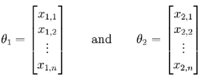
Their method involves the construction of m separate binomial distribution, where the time periods are denoted t₁, , , ,_{L L}t_i t_m, and have the set of a discrete stochastic for X , where _i X is only defined at time _i t . In general they have the _i

form of X at node r: _i

_{, 0} N ri r

i r i i

X = X u − d (4.1.5) where N_i =

∑

i_l=1n_l , and they have to determine the up and down movements , u d _{i i}

and the branching probabilities that satisfy the equations (4.1.2), (4.1.3) and (4.1.4). They denote

0

ln( / )

i i

x = X X

and the probabilities to reach x given a node _i x_i−1,r at t_i−1 as

1 1,

( |i i i r)

q x x₋ = x₋ or ( )q x _i

An example, where m=2 and we have X₀, X₁ and X is illustrated in Figure 1.  ₂

Lemma 1 Suppose that the up and down movements u and _i d are chosen so that _i

1 0 1, 1 2( ( ) / ) , 1, 2, , , 1 exp(2 ( ) / ) i N i i i i i i i E X X d i m t t n σ_{− −} = = + − L (4.1.6) 1 0 2( ( ) / )Ni , 1, 2, , , i i i u = E X X −d i= _L m       (4.1.7)

where

1

i i l l

N =

∑

₌ n , then if , for all i, the conditional probability ( )q x_l →0.5 as

l

n → ∞ , for l _{= L , then the unconditional mean and the conditional volatility of} 1, ,i

the approximated process approach respectively their true values:

1, 1, 0 0 1, , ˆ ( ) ( ) ˆ lim , lim l i i i i i i i n n l i E X E X X X σ− σ − →∞ →∞ = → → L  

Figure 1 A discrete process for X1, X2

There are n1+1 nodes at t1 numbered r = 0, 1,…, n1. There are n1+ n2+1 nodes at t2 numbered r = 0, 1,…,

n1+ n2. X0 is the starting price, X1 is the price at time t1, and X2 is the price at time t2. u1, d1, u2 and d2 are

the proportionate up and down movements.

Since x_i =ln(X X_i/ ₀) is normally distributed, it follows that the regression

1 , 1( ) 0 i i i i i i i x = +a b x₋ +ε E₋ ε = is linear with 2 2 2 [ ( ) ]/ b = tσ − −t t σ t σ ,

and

1

( ) ( )

i i i i

a =E x −b E x₋

They determined the conditional probabilities ( )q x so that _i

1( ) 1,

i i i i i r

E₋ x = +a b x₋

held for the approximated variables x and _i x_i−1.

Theorem 1 Suppose that the X are joint lognormally distributed. If the _i X are _i

approximated with binomial distributions with N_i =N_i−1+ stages and n_i u and _i d _i

given by equations (4.1.6) and (4.1.7), and if the conditional probability of an up movement at node r at time i−1 is

1, 1 1 1, ( ) ln ln ln ( | ) , , (ln ln ) ln ln i i i r i i i i i i i r i i i i i a b x N r u r d d q x x x i r n u d u d − − − − + − − − = = − ∀ − − (4.1.8) then ˆμ_i → and μ_i σˆ0,i →σ0,i and σˆi−1,i →σi−1,i as ni → ∞ ∀ , i

4.2 Applying the HSS Methodology to the LMM

After introducing the HSS methodology, we now apply this methodology into the LMM and make some change to satisfy our conventions. We have the following propositions.

Proposition 1 For the forward LIBOR rate which follows the lognormal distribution,

we can choose the proper up and down movements to determine the i-th period of the

n

T -maturity forward LIBOR rate and have the form

( ; , 1) (0; , 1) i , , , ,1 2

N r r

n n r n n i i n

f i T T₊ = f T T₊ u − d i T T= _L T (4.2.1) where

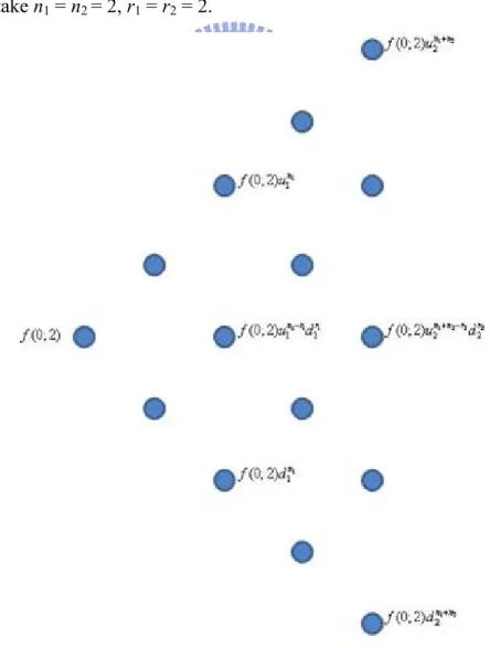
1 1 1 1, 1 2[ ( ( ; , )) / (0; , )] 1 exp(2 ( ) / ) i N n n n n i i i i i i E f i T T f T T d T T n σ ₋+ ₋ + = + − (4.2.2) u_i =2[ ( ( ; ,E f i T T_{n n+1})) / (0; ,f T T_{n n+1})]− (4.2.3) d_i 1 i i i N =N₋ + (4.2.4) n r: node’s number from top to bottom at time T _i

The structure of the binomial tree can be shown as Figure 2, with n₁+ nodes at 1

1

T numbered 0,1, … , . There are n n 1 nodes at T numbered ₂

1 2

0,1, ,

r= _K n +n . Here we write the forward rate 0; 2,3 in abbreviated form 0; 2 and take n1 = n2 = 2, r1 = r2 = 2.

After determining the structure of the forward LIBOR tree, we then have to choose the probability to satisfy the Proposition 1.

Proposition 2 Suppose that the forward LIBOR rate f i T T( ; ,_{n n+1}) are joint

lognormally distributed. If the f i T T( ; ,_{n n+1}), i T T= ₁, , ,_{2 L} T_n are approximated with binomial distributions with N_i =N_i−1+ stages and n_i u and _i d given by equations _i

(4.2.2) and (4.2.3), and if the conditional probability of an up movement at node r at time T is _i 1 1 1 1, ( ) ( ) ln ln ln ( | ) , (ln ln ) ln ln i i i i i i i i i r i i i i i E x N r u r d d q x x x i r n u d u d − − − − − − − = = − ∀ − − (4.2.5) where 1 1 ( ; , ) ln (0; , ) n n i n n f i T T x f T T + + = (4.2.6) Ei−1( )xi = +ai b xi i−1,r =E x( )i −b E xi ( i−1)+b xi i−1,r      (4.2.7)

For determining the conditional probability, it has some skills to use for the term of E_i−1( )x_i and following are the procedures to derive E_i−1( )x_i . We first derive

( )_i

E x term in equation (4.2.7). Since the forward rate f i T T( ; ,_{n n+1}) is lognormally distributed, we have 1 2 0, 1 ( ( ; , )) 1 ( ) ln[ ] (0; , ) 2 n n i i n n E f i T T E x f T T σ + + = − (4.2.8) Second, we use the result of equation (3.2.7) obtained from the last section, and rewrite it as follows: 1 1 1 1 2 2 2 3 1, 2, 1 1 1 2 2 2 3 1 , 1 [ ( ; , )] ( ; , ) ( ; , ) 1 ( ; , ) 1 ( ; , ) 1 ( ; , ) ( ; , ) 1 ( ; , ) t n n n n n n n n n n n n n n E f T T T f t T T f t T T f t T T f t T T f t T T f t T T f t T T δ δ _{σ σ} δ δ δ _σ δ + + + + = + ⋅ + ⋅ + + + + ⋅ + % % % L (4.2.9)

form of E f T T T_t( ( ; ,_{1 n n+1})) / (0; ,f T T_{n n+1}): 1 1 1 1 1 1 1 1 2 2 2 3 1 1, 2, , 1 1 1 2 2 2 3 1 ( ; , ) [ ( ; , )] (0; , ) ( ; , ) ( ; , ) ( ; , ) ( ; , ) ( ; , ) (1 ) (0; , ) 1 ( ; , ) 1 ( ; , ) 1 ( ; , ) n n t n n n n n n n n n n n n n n n n n n n n f t T T E f T T T f T T f t T T f t T T f t T T f t T T f t T T f T T f t T T f t T T f t T T δ δ δ _{σ σ σ} δ δ δ + + + + + + + + × = × + ⋅ + ⋅ + + ⋅ + % + % L + % (4.2.9) Finally, we substitute it into the formula (4.2.8) to obtain ( )E x term. Then, we _i

take the value of ( )E x into equation (4.2.7) to compute the up movement _i

probability at time T given the node _i f i( 1; ,− T T_{n n+1})_r.

Note that when nl stages approach the infinite l= L , the sum of n1, ,i l stages

also approach the infinite (i.e.

1

i i l l

N =

∑

₌ n → ∞). We can reduce the up and down movements to the briefer form which is easier to calculate. That is

1, 1 2 1 exp(2 ( ) / ) i i i i i i d T T n σ _{− −} = + − 2 i i u = − d

5 The Pricing of the Interest Rate Derivatives in the LMM

After we construct the forward tree process, it can be employed to price the derivatives. By beginning from the bond option on zero coupon bond (ZCB), then extend to the caplets.

5.1 The valuation of bond option on zero coupon bond in LMM

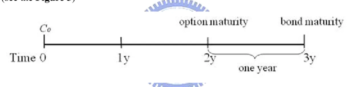
The bond option on ZCB is a bond that can be callable before maturity date with a callable price K. For example, we have a three years maturity zero coupon bond with a callable value K equal to 0.952381 dollar at year two. That is to say we can redeem the ZCB at year two with 0.952381 dollar or hold it until maturity at year three with 1 dollar. Therefore, we have to price the option value C0 of this callable bond at time 0

(see the Figure 3)

Figure 3 The callable bond for the 3 year maturity ZCB

To obtain the callable bond option value, we use the lattice method to price the option value of the callable bond. To get the payoff function at year two, we need know the zero coupon price at year two maturity at year three (i.e. P(2,3)). Comparing to the callable value K, we take function max(P(2,3)-K,0). Then we discount it back to the time 0 to get the option value of the callable bond. Here we take the flat forward rate 5% and constant volatility 10% and have

0 (0, 2) [max( (2,3) , 0)] 0.90702948 0.00258128 0.00234130 C =P ×E P −K = × =

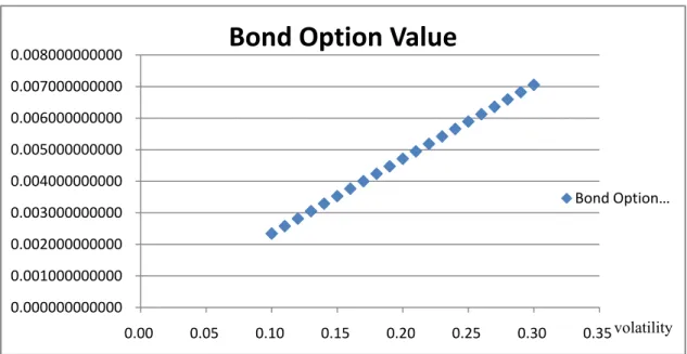
After having the option value at 10%volatility, we increase the volatility until reach 30% to see the relationship between option value and volatility. We plot the

results into Figure 4 to see the trend between option values and volatility.

Figure 4 Bond option values for different volatility

From the above figure, we find that when the volatility increases, the value of bond option on ZCB increases. It is consistent with the inference for the Greek letter

vega when the underlying asset’s volatility increases the option value increases, too.

5.2 The valuation of caplets in LMM

A popular fixed income security is an interest rate cap, a contract that pays the difference between a variable interest rate applied to a principal and a fixed interest rate (strike price) applied to the same principal whenever the variable interest rate exceeds the fixed rate. We consider a cap with total life of T and let the tenor δ , the notional value A and the strike price K be fixed positive values. Note that the reset dates are T1, T2, … , Tn and define Tn+1 = T. Define the forward rate

1

( ; ,_{i i i} )

f T T T₊ as the future spot interest rate for the period between T and _i T_i+1

observed at time T (1_i ≤ ≤ . The payoff function of a caplet at time i n) T_i+1 is A× ×δ max( ( ; ,f T T T_{i i i+1})−K,0) (5.2.1)

Equation (5.2.1) is a caplet on the spot rate observed at time T with payoff _i

0.000000000000  0.001000000000  0.002000000000  0.003000000000  0.004000000000  0.005000000000  0.006000000000  0.007000000000  0.008000000000  0.00  0.05  0.10  0.15  0.20  0.25  0.30  0.35 

Bond Option Value

Bond Option … volatility

occurring at time T_i+1. The cap is a portfolio consisted of n such call options which the underlying is known as caplet.

To derive out the price of the cap, we have to price the caplet first and then sum up the n caplets value to get the price of a cap. For a caplet price at time t, we use the Black’s formula mentioned in chapter 3 (Equation (3.1.4)) to get the theoretical value. Thus, we restate the as follows:

caplet t_i( )= × ×A δ_i P t T( , _i+1)[ ( ; ,f t T T_{i i+1}) ( )N d₁ −KN d( )]₂ (5.2.2) where 2 1 1 2 1 2 ln( ( ; , ) / ) ( ) / 2 , ln( ( ; , ) / ) ( ) / 2 , i i i i i i i i i i i i f t T T K T t d T t f t T T K T t d T t σ σ σ σ + + + − = − − − = −

After having the theoretical value as our benchmark, we use the payoff function to compute the price in the lattice method. To get the payoff function at time T_i+1, we have to know the evolution of the forward rate f(0; ,T T_{i i+1}) at time T . We construct _i

the binomial tree of f(0; ,T T_{i i+1}) and known the ( ( ; ,f T T T_{i i i 1})_r K)+

+ − , r = 0, 1, …, i.

Calculating the expectation of the payoff at time T_i+1, and then multiple the ZCB of

1

( , _i )

P t T₊ to get the caplet value at time t.

In the followings, we take the 10 maturity of cap to compute the individual caplet from 1 period to 10 periods with the assumption of tenor δ and notional value A are equal to one and the volatility is constant and equal to 10%. Here the strike price K is 5%, the forward curve is flat 5% and the stages ni for every period are

1(0) (0, 2) [max( (1;1, 2) ,0)] 1 1 (0, 2) 0.0020112666 0.90702948 0.0020112666 0.0018242781 caplet A P E f K P

δ

= × × × − = ⋅ ⋅ ⋅ = ⋅ =

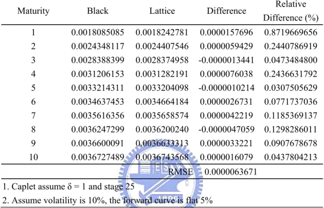
Table 1 Volatility is 10% and Stage ni for Every Period is 25

Maturity Black Lattice Difference Relative Difference (%) 1 0.0018085085 0.0018242781 0.0000157696 0.8719669656 2 0.0024348117 0.0024407546 0.0000059429 0.2440786919 3 0.0028388399 0.0028374958 -0.0000013441 0.0473484800 4 0.0031206153 0.0031282191 0.0000076038 0.2436631792 5 0.0033214311 0.0033204098 -0.0000010214 0.0307505629 6 0.0034637453 0.0034664184 0.0000026731 0.0771737036 7 0.0035616356 0.0035658574 0.0000042219 0.1185369137 8 0.0036247299 0.0036200240 -0.0000047059 0.1298286011 9 0.0036600091 0.0036633313 0.0000033221 0.0907678678 10 0.0036727489 0.0036743568 0.0000016079 0.0437804213 RMSE 0.0000063671

1. Caplet assume δ = 1 and stage 25

2. Assume volatility is 10%, the forward curve is flat 5%

Table 1 is the results for different maturity caplets. Besides the relative

difference, we also use the RMSE to see the difference between the lattice value and Black’s model for the whole maturity. The definition of the RMSE is given as follows:

RMSE (Root Mean Square Error)

A frequently-used measure of the differences between values predicted by a model or an estimator and the values actually observed from the thing being modeled or estimated. For the comparing difference between two models, the formula of RMSE can be expressed as

2 1, 2, 2 1 1 2 1 2 1 2 ( ) ( , ) ( , ) (( ) ) n i i i x x RMSE MSE E n θ θ ₌ θ θ ₌ θ θ_{− =}

∑

= − where

Here, θ1 and θ2 represent the lattice value and Black’s model respectively which

maturity form one to ten.

Now we change the stages from 25 to 50 to figure out the relationship between stages and RMSE. The results are shown in Table 2.

Table 2 Volatility is 10% and Stage ni for Every Period is 50

Maturity Black Lattice Difference Relative Difference (%) 1 0.0018085085 0.0018099405 0.0000014320 0.0791823392 2 0.0024348117 0.0024397802 0.0000049685 0.2040608652 3 0.0028388399 0.0028434461 0.0000046061 0.1622542164 4 0.0031206153 0.0031230795 0.0000024643 0.0789673074 5 0.0033214311 0.0033207434 -0.0000006878 0.0207066243 6 0.0034637453 0.0034620815 -0.0000016638 0.0480341136 7 0.0035616356 0.0035626664 0.0000010308 0.0289416315 8 0.0036247299 0.0036267433 0.0000020134 0.0555455781 9 0.0036600091 0.0036617883 0.0000017792 0.0486107386 10 0.0036727489 0.0036734197 0.0000006708 0.0182649876 RMSE 0.0000025690 1. Caplet assume δ = 1 and stage 50

2. Assume volatility is 10%, the forward curve is flat 5%

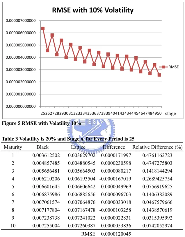
We also plot the RMSE with different stages between periods from 25 to 50 to see the convergence behavior of RMSE. Figure 5 shows that the convergence behavior of RMSE for the different stages. We find that when we increase stages between periods, both relative difference and RMSE decrease and RMSE converge to zero with the stages go to infinite.

To see the impact of volatility on the value of different caplets and the convergence behavior of RMSE, we change the volatility from 10% to 20%. We do the same procedures as we do in volatility 10%, and results for the 25 and 50 stages

are presented in Table 3 and Table 4 respectively. Finally, we plot the RMSE with different stages from 25 to 50 for volatility 20% in Figure 6.

Figure 5 RMSE with Volatility 10%

Table 3 Volatility is 20% and Stage ni for Every Period is 25

Maturity Black Lattice Difference Relative Difference (%) 1 0.003612502 0.003629702 0.0000171997 0.4761162723 2 0.004857485 0.004880545 0.0000230598 0.4747275803 3 0.005656481 0.005664503 0.0000080217 0.1418144294 4 0.006210206 0.006193504 -0.0000167019 0.2689425754 5 0.006601645 0.006606642 0.0000049969 0.0756919625 6 0.006875986 0.006885656 0.0000096703 0.1406382089 7 0.007061574 0.007064876 0.0000033018 0.0467579666 8 0.007177804 0.007167478 -0.0000103258 0.1438570619 9 0.007238738 0.007241022 0.0000022831 0.0315395992 10 0.007255004 0.007260387 0.0000053836 0.0742052974 RMSE 0.0000120045 1. Caplet assume δ = 1 and stage 25

2. Assume volatility is 20%, the forward curve is flat 5% 0.000000000000  0.000001000000  0.000002000000  0.000003000000  0.000004000000  0.000005000000  0.000006000000  0.000007000000  2526272829303132333435363738394041424344454647484950

RMSE with 10% Volatility

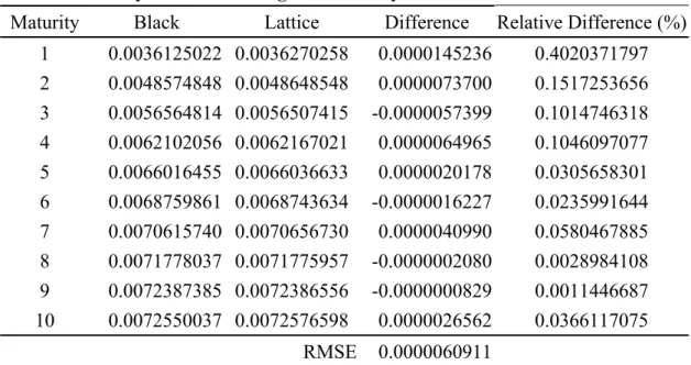
RMSE stage

Table 4 Volatility is 20% and Stage ni for Every Period is 50

Maturity Black Lattice Difference Relative Difference (%) 1 0.0036125022 0.0036270258 0.0000145236 0.4020371797 2 0.0048574848 0.0048648548 0.0000073700 0.1517253656 3 0.0056564814 0.0056507415 -0.0000057399 0.1014746318 4 0.0062102056 0.0062167021 0.0000064965 0.1046097077 5 0.0066016455 0.0066036633 0.0000020178 0.0305658301 6 0.0068759861 0.0068743634 -0.0000016227 0.0235991644 7 0.0070615740 0.0070656730 0.0000040990 0.0580467885 8 0.0071778037 0.0071775957 -0.0000002080 0.0028984108 9 0.0072387385 0.0072386556 -0.0000000829 0.0011446687 10 0.0072550037 0.0072576598 0.0000026562 0.0366117075 RMSE 0.0000060911

1. Caplet assume δ = 1 and stage 50

2. Assume volatility is 20%, the forward curve is flat 5%

Figure 6 RMSE with Volatility 20%

We find that with the volatility increases, the value of caplets increases, and the convergence rate of RMSE decreases. It is consistent with high volatility makes the option value more valuable and convergence rate slower.

0.000000000000  0.000002000000  0.000004000000  0.000006000000  0.000008000000  0.000010000000  0.000012000000  0.000014000000  2526272829303132333435363738394041424344454647484950

RMSE with 20%Volatility

RMSE stage

6 Conclusions

To implement the LIBOR market model, we construct a recombining binomial tree to depict the evolution of the forward LIBOR rate. In this model, we have all the forward rates for the whole maturity at any node of the recombining binomial tree. With these rates, we can easily figure out the early exercise decision for the American style derivatives which is a tough work in the Monte Carlo simulation.

After constructing the recombining binomial tree, the payoff of the interest rate derivatives on each node can be obtained. The pricing procedures of the derivatives can be calculated by backward induction with the conditional probability. We use the proposed model to calculate the value of bond option on zero coupon bond and caplets. Comparing to the theoretical value, we find the theoretical value and lattice method is close. However, with the stage between period by period increases, the difference between theoretical value and lattice method decreases. Besides, as the volatility increases the converge rate of RMSE decrease.

In the future, we have to find out the joint probability between different maturity forward rates and adjust the stages between period by period to fit the strike price to reduce the nonlinearity error. Trying to change the constant volatility to stochastic volatility to fit the volatility term structure will make the model more complete.

References

Brace, A., D. Gatarek, and M. Musiela, 1997, “The Market Model of Interest Rate Dynamics.” Mathematical Finance, 7, no. 2, 127-155

Brigo D., F. Mercurio, 2006, Interest Rate Models - Theory and Practice with Smile,

Inflation and Credit, 2nd Edition, Springer.

Cox, J. C., J. E. Ingersoll, and S. A. Ross, 1985, “A Theory of the Term Structure of Interest Rates.” Econometrica, 53, 385-407

Derrick, S., D. Stapleton and R. Stapleton, 2005, “The Libor Market Model: A Recombining Binomial Tree Methodology.” Working paper

Health, D., R. A. Jarrow, and A. Morton, 1990, “Bond Pricing and the Term Structure of Interest Rates: A Discrete Time Approximation.” Journal of Financial and

Quantitative Analysis, 25, no. 4, 419-440

Health, D., R. A. Jarrow, and A. Morton, 1992, “Bond Pricing and the Term Structure of Interest Rates: A New Methodology.” Econometrica, 60, no. 1, 77-105 Ho, T. S. Y., and S.-B. Lee, 1986, “Term Structure Movements and Pricing Interest

Rate Contingent Claims.” Journal of Finance, 41, 1011-1029

Ho, T.S., R.C. Stapleton, and M.G. Subrahmanyam, 1995, “Multivariate Binomial Approximations for Asset Prices with Non-Stationary Variance and Covariance Characteristics,” Review of Financial Studies, 8, 1125-1152.

Hull, J., 2006, Options, Futures and Other Derivative Securities, 6th Edition, Pearson. Hull, J. and A. White, 1990, “Pricing Interest Rate Derivative Securities.” Review of

Financial Studies, 3, no. 4, 573-592

Hull, J. and A. White, 1993, “Bond Option Pricing Based on a Model for the Evolution of Bond Prices.” Advances in Futures and Options Research, 6, 1-13

Hull, J. and A. White, 1993, “The Pricing of Options on Interest Rate Caps and Floors Using the Hull-White Model.” Journal of Financial Engineering, 2, no. 3, 287-296

Hull, J. and A. White, 1994, “Numerical Procedures for Implementing Term Structure Model I：Single Factor Models.” Journal of Derivatives, 2, 7-16

Hull, J. and A. White, 1996, “Using Hull-White Interest Rate Trees.” Journal of

Derivatives, 26-36

Hull, J. and A. White, 2000, “Forward Rate Volatilities, Swap Rate Volatilities, and the Implementation of the LIBOR Market Model.” Journal of Fixed Income, 10, no. 2, 46-62

Jamshidian, F., 1989, “An Exact Bond Option Formula.” Journal of Finance, 44, 205-209

Jamshidian, F., 1997, “LIBOR and Swap Market Models and Measures.” Finance and

Stochastics, 1, 293-330

Miltersen, K., K. Sandmann, and D. Sondermann, 1997, “Closed Form Solutions for Term Structure Derivatives with Lognormal Interest Rates.” Journal of Finance, 52, no. 1, 409-430

Nawalkha, S., N. A. Beliaeva and G. M. Soto, 2007, Dynamic Term Structure

Modeling, Wiley.

Poon, S.H. and R.C. Stapleton, 2005, Asset Pricing in Discrete Time A Complete

Markets Approach, Oxford.

Rebonato R., 2002, Modern Pricing of Interest-Rate Derivatives: The LIBOR Market

Model and Beyond, Princeton University Press.

Vasicek, O. A., 1977, “An Equilibrium Characterization of the Term Structure.”