兩條平行河川間自由水層因抽水所引起的三維地下水流通解

(1)

國立交通大學

環境工程研究所

博士論文

兩條平行河川間自由水層因抽水所引起的三維地下水

流通解

A General Analytical Solution for Three-Dimensional

Groundwater Flow Induced by Pumping in Unconfined Aquifers

Bounded by Two Parallel Streams

研究生：黃璟勝

指導教授：葉弘德

(2)

兩條平行河川間自由水層因抽水所引起的三維地下水

流通解

A General Analytical Solution for Three-Dimensional

Groundwater Flow Induced by Pumping in Unconfined Aquifers

Bounded by Two Parallel Streams

研究生：黃璟勝 (

Ching-Sheng Huang

)

指導教授：葉弘德 (

Hund-Der Yeh

)

國立交通大學

環境工程研究所

博士論文

A Dissertation

Submitted to Institute of Environmental Engineering

College of Engineering

National Chiao Tung University

in Partial Fulfillment of the Requirements

for the Degree of

Doctor of Philosophy

in

Environmental Engineering

January, 2013

Hsinchu, Taiwan

中華民國一百零二年二月

(3)

兩條平行河川間自由水層因抽水所引起的三維地下水

流通解

研究生：黃璟勝指導教授：葉弘德

國立交通大學環境工程研究所

摘要

本研究發展一個數學模式，用以描述在兩條平行河川之間的自由含水層，因抽水井所引起的三維地下水流之解析解。所建構的數學模式，包含一個新的地下水流控制方程式，使所發展的解析解可適用於三種抽水井，包含垂直井、水平井、及輻射收集井；接著採用自由液面方程式，描述液面因抽水而產生的洩降，並以第三類邊界條件代表兩條平行河川的低透水性河床。應用積分轉換的方法，推導出此數學模式的水力水頭解析解，此解由含特徵函數的三階無限級數所組成，其特徵值的計算需用到尋根法；我們提出一個解析公式用來求適當的初始猜值，配合牛頓法可有效率地求出特徵值。依據達西定律和水頭解析解，可導出描述河川滲入率(stream depletion rate, SDR)的解析解，此解析解對現地的水平井或輻射收集井的預測，可與現地問題量測的結果相吻合。依據解析解的模擬結果，我們得到以下的結論：未受壓含水層中的重力排水對 SDR 有顯著的影響，在抽水中期， SDR 不隨抽水時間增加而增加，若忽略水頭垂直方向的變化，會顯著地高估

SDR，此結論和紐西蘭 Doyleston 附近的現地實驗結果一致。此外，輻射收集井的側臂分布對於洩降有顯著的影響，在河川滲入行為發生之前，最大洩降位於在

(4)

輻射井的中心；當河水開始滲入含水層，最大洩降開始遠離井中心並往內陸方向移動。

關鍵字：垂直井、水平井、輻射收集井、受壓含水層、自由液面方程式、河川滲入率(SDR)、二重積分轉換、有限複立葉餘弦轉換、拉普拉斯轉換

(5)

A General Analytical Solution for Three-Dimensional Groundwater

Flow Induced by Pumping in Unconfined Aquifers Bounded by Two

Parallel Streams

Student：Ching-Sheng Huang Adviser：Hund-Der Yeh Institute of Environmental Engineering

National Chiao Tung University

ABSTRACT

This thesis develops a mathematical model for describing three-dimensional groundwater flow induced from a vertical well, horizontal well or radial collector well (RC well) in an unconfined aquifer bounded by two parallel streams. A new governing equation with a sink term standing for the well is presented. A simplified free surface equation is used to describe the depletion of water table in the aquifer. The third-type boundary condition is employed for the boundary condition at the interface where a low-permeability streambed is connected to the aquifer. The aquifer we concern is of finite extent; therefore, the head solution of the model, derived by integral transforms, can be expressed in terms of an infinite series with eigenvalues requiring a root-finding scheme such as Newton method. An analytical expression is developed to give initial guesses for the eigenvalues. The solution for stream depletion rate (SDR) describing filtration rate from the streams is acquired based on Darcy’s law and the head solution. The present solution is applied to predict the hydraulic head near a horizontal well or a RC well for the real-world cases. The predicted results are reasonable when compared with the field observed data. With the aid of the present solution, we have found that the gravity drainage of an unconfined aquifer has

(6)

significant effects on temporal SDR. The curve of temporal SDR tends to be flat due to the gravity drainage during the middle period of pumping time. The vertical groundwater flow described by the free surface equation should be used even for the case of a fully-penetrating well. The SDR will be overestimated if neglecting the vertical flow in the model. Such a result is confirmed by the comparison of SDR predicted from the present solution with that taken from a field SDR experiment executed near Doyleston in New Zealand. Additionally, lateral configurations of a RC well have significant effects on spatial drawdown distributions. The largest drawdown occurs right at the center of a RC well before the filtration and moves landward once the filtration starts to recharge the aquifer.

KEYWORDS: vertical well, horizontal well, radial collector well, confined aquifer,

free surface equation, stream depletion/filtration rate (SDR), double-integral transform, finite Fourier cosine transform, Laplace transform

(7)

誌謝

本論文承蒙葉弘德教授的細心指導，才能順利完成，在此對我的恩師葉老師致上最深的謝意。口試期間，中央大學的葉高次教授及陳瑞昇教授、逢甲大學的馮秋霞教授、萬能科技大學的楊紹洋教授和交通大學的傅武雄教授給予的建議，使本論文內容更加充實完備，在此一併致謝。博士班期間，葉弘德教授除了將專業知識傾囊相授之外，對於研究應有的態度和行為，更以身作則。葉老師對於目標努力不懈的毅力，讓我深感佩服。感謝葉老師和國科會提供參加國外研討會的機會，讓我確認自己的努力方向並拓展視野；感謝語言中心的吳思葦老師，教導我英語報告的技巧；感謝學姐張雅琪，在我剛踏入研究領域時，提供適時的協助；感謝學長李珖儀，幫助我完成資格考和口試；此外，感謝同屆的同學陳庚轅、鄒佩蓉和學弟妹們，讓我的研究生涯更多采多姿。最後，感謝父母親的支持，讓我能專心於學業上；感謝弟弟在家中的幫忙，讓我能更專注於學業；此外，感謝台灣社會的人們，默默地提供我每天的需求，便利了我在學校的生活。

(8)

LIST OF TABLES

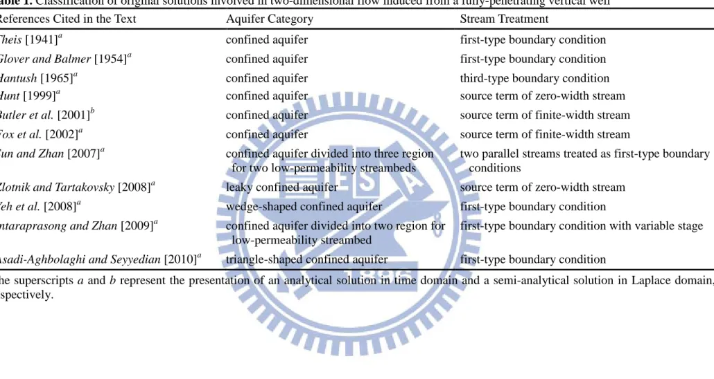
Table 1. Classification of original solutions involved in two-dimensional flow induced

from a fully-penetrating vertical well………51

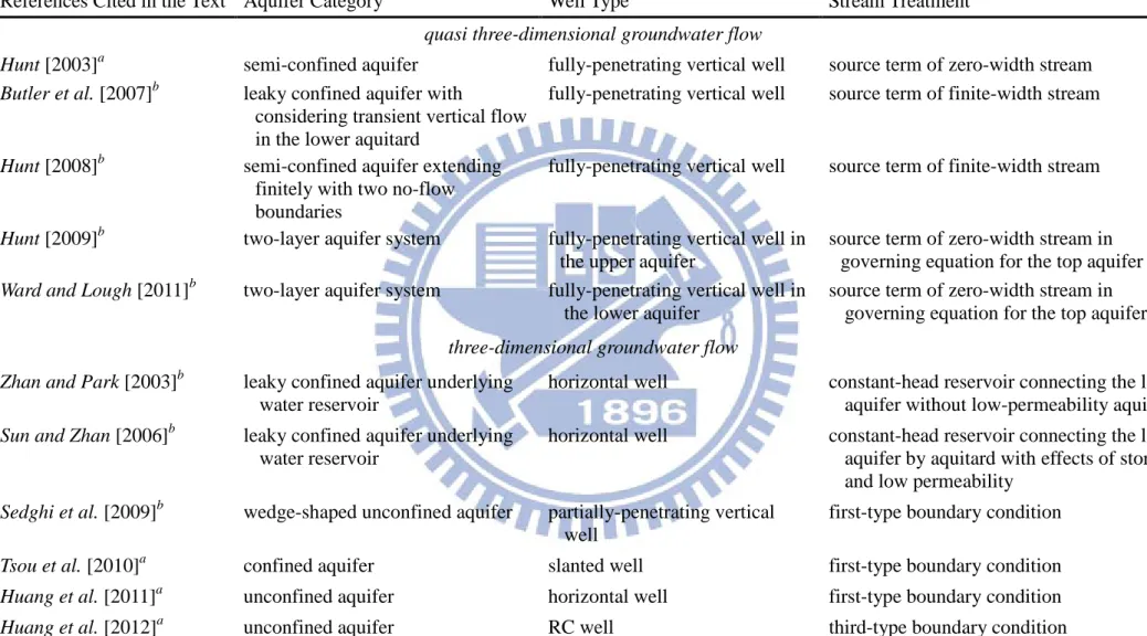
Table 2. Classification of original solutions involved in quasi three-dimensional and

three-dimensional flow………..52

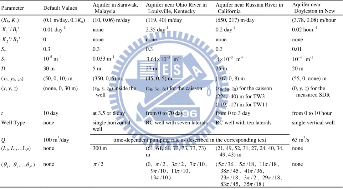
Table 3. The default values and field data for aquifer parameters and well

(11)

LIST OF FIGURES

Figure 1. Schematic diagram of an unconfined aquifer with a vertical well or a radial

collector well; (a) and (c) top view; (b) and (d) cross section view………...54

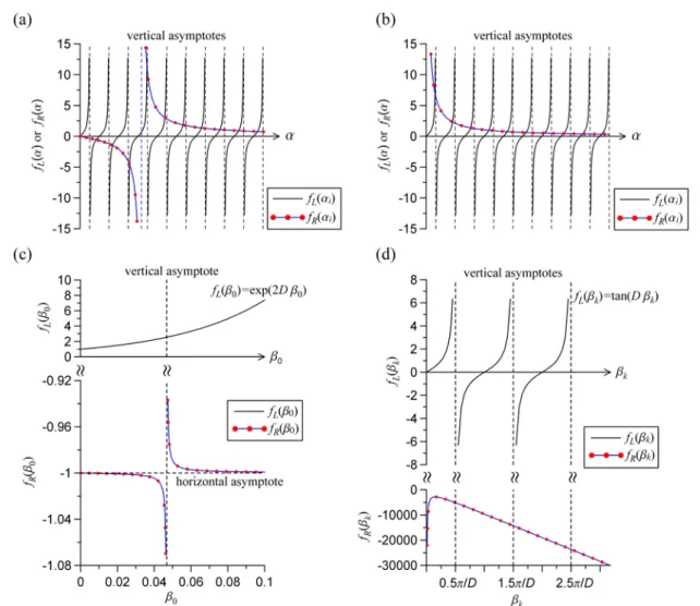
Figure 2. The patterns of the LHS and RHS functions from equation (20) for (a)

0 '

2 ≠

K and (b) K₂'=0 as well as from (c) equation (21) and (d) equation (22)...55

Figure 3. Contours of spatial head distributions induced from a fully-penetrating

vertical well for various Sy/Kv when t=10 m/day………56

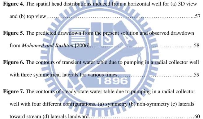
Figure 4. The spatial head distributions induced from a horizontal well for (a) 3D view

and (b) top view………...57

Figure 5. The predicted drawdown from the present solution and observed drawdown

from Mohamed and Rushton [2006]………...58

Figure 6. The contours of transient water table due to pumping in a radial collector well

with three symmetrical laterals for various times………...59

Figure 7. The contours of steady-state water table due to pumping in a radial collector

well with four different configurations. (a) symmetry (b) non-symmetry (c) laterals toward stream (d) laterals landward………60

Figure 8. Temporal distribution curves of SDR for four different lateral configurations

61

Figure 9. Water levels predicted by the present solution and the observed field data from

Schafer [2006]……….62

Figure 10. Water levels predicted by the present solution and the observed field data from

(12)

Figure 12. Steady-state water table distributions at y=0 for various K /1' K_h………...65

Figure 13. Temporal distribution curves of SDR for the LHS stream for various

h

K

K /₁' _{………..66}

Figure 14. Temporal distribution curves of SDR due to pumping in a radial collector

well with three symmetrical laterals for various K /_v K_h_……….67

Figure 15. Temporal distribution curves of SDR for various lateral number and length

68

Figure 16. Comparison of temporal SDR predicted from the present solution, Theis’

solution [1941] and Hantush’s solution [1965] with field data taken from a field SDR experiment executed by Hunt et al. [2001]………69

(13)

NOTATION

h : hydraulic head in an aquifer

(x, y, z) : variables of Cartesian coordinate where x axis is perpendicular to streams

t : time (Kh, Kv)

: hydraulic conductivity in the horizontal and vertical direction, respectively

Sy : specific yield

Ss : specific storage

(Wx, Wy) : aquifer width in x and y direction, respectively

D : aquifer thickness

T : transmissivity (Kh D)

S : storage coefficient (Ss D)

(K , 1' B ) 1' : streambed hydraulic conductivity and its thickness, respectively, on the

left hand side of an aquifer

1

c : K₁'/(K_hB₁')

(K , ₂' B ) : streambed hydraulic conductivity and its thickness, respectively, on the ₂' right hand side of an aquifer

2

c : K₂'/(K_hB₂')

Q : pumping rate

N : the number of laterals

(x0, y0) : location of vertical well or the center of radial collector well

z0 : elevation of horizontal well or radial collector well

(Ln, θ ) n : length and counterclockwise angle from x axis, respectively, for the n-th

lateral )

, ,

(14)

CHAPTER 1 INTRODUCTION 1.1. Background

Groundwater depletion, a key issue associated with groundwater supplies, has been

increasing rapidly and inevitably as a result of industrial development and growing

population since the past haft century [e.g., Konikow and Kendy, 2005; Zume and

Tarhule, 2008; Kim, 2010; Ravazzani et al., 2011]. The average rate of groundwater

consumption is estimated in the range of 750-800 km3/year in the whole world [Shah et

al., 2000]. Groundwater withdrawals will induce a considerable amount of filtration

from a reservoir to its adjacent aquifer if an abstraction well is installed near the

reservoir. Therefore, it is worthy to review the effects of groundwater withdrawals on

some issues such as aquatic ecosystem near streams, water quality for agricultural

irrigation, distributions of water rights, and utilization for households and industries.

Aquatic ecosystem near a stream will be damaged if the stream stage declines

excessively due to a large quantity of filtration [Wen and Chen, 2006]. The balance of

food chain could be destroyed if a specific species is removed. Some hydrophytes are,

for example, not survival in the absence of a high-level stream stage, and herbivores are

jointly not, either.

Groundwater abstractions for agricultural irrigation could become contaminated

(15)

amount of groundwater is withdrawn, and the contaminants enter the aquifer through

filtration. During rainy seasons, the contaminants are remained in the aquifer even when

pumping from wells ceases. After several alternations between drought and rainy

seasons, the contaminants may eventually reach the abstraction wells, and in turn

degrade the quality of pumped groundwater.

Groundwater recharge from two different surfaces sources such as streams is

involved in distribution of water from surfaces sources regulated by water rights. The

contribution to groundwater abstraction for a well comes from two streams. Generally

speaking, most of the groundwater is contributed from the neighboring stream. However,

under some conditions, all of the groundwater may be extracted almost from the other

stream far away from the abstraction well. Accordingly, an accurate estimate of

filtration rate plays an important role for hydrologists in the managements of water

resources.

In the past, to meet the water demand for domestic and industrial, dams had been

used for storage of surface water in providing more consistent supplies. However, a

suitable site for dam construction is scanty. Recently, awareness of environmental and

ecological consciousness has resulted in dam removals. Groundwater utilization

therefore becomes inevitable.

(16)

land subsidence. During the early period of pumping time, the filtration recharges the

adjacent aquifer with parts of the groundwater extraction. The drawdown increases with

time due to the loss of the groundwater. During the late period, the stream water

filtration balances the groundwater withdrawal, and the drawdown becomes stabilized.

1.2. Radial Collector Well (RC Well)

Radial collector wells (RC wells) have been commonly designed and used to

collect water from a nearby stream. The RC well designed by Ranney Leo was

developed from horizontal wells in 1930s [Hunt, 2006]. A RC well generally comprises

a central reinforced concrete caisson and several laterals under the ground surface. The

central caisson is drilled downward with an inside diameter ranging from 3 to 6 m or

larger, and the laterals horizontally extend from the central caisson at a proper depth in

an aquifer. The advances in well-drilling techniques provide more practical guidance on

well installations in aquifers. The groundwater moves through the laterals to the caisson

if the RC well starts pumping.

The magnitude of drawdown can be controlled artificially by adopting a RC well

with several laterals. Compared with a traditional vertical well, for the same pumping

rate, the RC well extracts groundwater from a wider range by extended horizontal

laterals. The drawdown can thus be minimized as small as possible. However, the length

(17)

accordingly determined based on the natural situation of aquifer thickness.

1.3. Review of Previous Solutions

A variety of analytical and semi-analytical solutions have been developed to assess

stream filtration induced from pumping under the condition of a fully-penetrating

stream. They can be classified according to the dimensions of groundwater flow, namely,

two-dimensional (2-D) flow, quasi three-dimensional (quasi 3-D) flow, and

three-dimensional (3-D) flow, as shown in the following three sections, respectively.

1.3.1. Two-Dimensional Flow

Most of the solutions have been developed considering 2-D groundwater flow

induced by a fully-penetrating well in a confined aquifer or a leaky confined aquifer

with a nearby stream. Theis [1941] was the first to propose an analytical solution for

stream filtration in a confined aquifer. The aquifer extends infinitely in the horizontal

direction, and the stream generated without a low-permeability streambed by

image-well theory is actually subject to a first-type boundary condition. The solution is

expressed in terms of an improper integration. Glover and Balmer [1954] simplified

Theis’ solution [1941] to a concise expression in terms of a complementary error

function. Hantush [1965] considered the same situations as Theis [1941] but under a

third-type stream boundary condition with a low-permeability streambed, and developed

(18)

The stream is commonly regarded as a source term in the governing equation. The

source term is expressed in terms of the Dirac delta function, representing a zero width

stream. Those solutions to the equation with a source term are applicable to the case of a

low-permeability streambed. On the other hand, the stream is treated as a line source for

the fully-penetrating stream under Dupuit assumption [Sun and Zhan, 2007]. Hunt’s

solution [1999] might be the first analytical solution derived by treating the stream as

the line source for a confined aquifer and was shown to be exactly the same as

Hantush’s solution [1965] according to Sun and Zhan [2007]. His solution is valid for

the whole domain of the aquifer divided by the stream because of the treatment of a

stream as a source term. In contrast, based on the treatment of the stream as a boundary,

Hantush’ solution [1965] is limited to the case of the side where a well is installed.

Additionally, Zlotnik and Tartakovsky [2008] also treated a stream as the line source but

considered a leaky confined aquifer. They presented an analytical solution for hydraulic

head and stream filtration.

To account for the effect of stream width on the model, some researchers divide an

aquifer into three zones with different governing equations. The middle zone has a

width equaling the stream width. Only the side zone has a fully-penetrating well treated

as a sink term in the governing equation. Those three governing equations are coupled

(19)

middle zone and side zones. Butler et al. [2001] used this approach to derive a

semi-analytical solution in Laplace domain for a confined aquifer and analyzed the

effect of stream width on stream filtration. Fox et al. [2002] considered the same model

as Butler et al. [2001] and derived an analytical solution in time domain.

Some articles are proposed to treat a stream as a first-type boundary condition for a

wedge-shaped aquifer or a triangle confined aquifer. Yeh et al. [2008] developed an

analytical solution for describing temporal head distribution and stream filtration for a

wedge-shaped aquifer bounded by a stream. For the triangle aquifer, Asadi-Aghbolaghi

and Seyyedian [2010] derived an analytical solution for steady-state head distributions

in the finite aquifer where two of the sides are a first-type stream boundary and the other

side is either a first-type boundary or a no-flow boundary.

Most of the articles adopted a third-type stream boundary as a stream boundary in

which the streambed permeability is considered but its storage is neglected. To account

for the storage effects, some articles considered the role of a streambed in the different

way. The streambed is treated as parts of an aquifer rather than parts of the boundary

and has different permeability and storage from the adjacent aquifer. One-dimensional

(1-D) groundwater flow which is perpendicular to the stream is considered in the

streambed. Under this situation, Sun and Zhan [2007] considered two parallel streams

(20)

the distributions of stream filtration from these two streams with different hydraulic

parameters. Intaraprasong and Zhan [2009] considered a temporal and spatial variation

in stream stage and derived a semi-analytical solution for quantifying the effect of the

variable stage on stream filtration.

The solutions mentioned above are summarized in Table 1. All of these solutions

account for the effect of 2-D flow induced by a fully-penetrating vertical well and can

be categorized based on the aquifer types and stream treatments.

1.3.2. Quasi Three-Dimensional Flow

Quasi 3-D flow model represents a multiple-layered aquifer system in which the

flow in the aquifer is horizontal and in the aquitard is vertical. The flow in the aquifer

system is coupled through the leakage term in their governing equations. The aquifer

system is classified herein into a semi-confined aquifer, leaky confined aquifer, and

two-layer aquifer system. Firstly, a semi-confined aquifer consists of a main aquifer and

a semi-permeable confining unit on the top. The groundwater flow in the unit is treated

to be vertical as a result of its thin thickness. Hunt [2003] developed an analytical

solution for head and stream filtration in such a semi-confined aquifer. The stream is

treated as the source term of zero width. Hunt [2008] also considered a semi-confined

aquifer but considered the stream as the source term of finite width. The aquifer extends

(21)

perpendicular to the stream. He developed a semi-analytical solution for hydraulic head

and stream filtration. Secondly, a leaky confined aquifer herein contains a main aquifer

and the aquitard at the bottom. The aquitard has only vertical flow due to its thin

thickness. Butler et al. [2007] derived a semi-analytical solution describing hydraulic

head and stream filtration for such an aquifer. Thirdly, a two-layer aquifer system

represents that each aquifer has horizontal flow and is coupled with the other one by the

leakage term in the governing equation. Hunt [2009] developed a semi-analytical

solution for such a aquifer system. The stream is treated as a source term of zero width,

and the vertical well fully penetrates the upper aquifer. Ward and Lough [2011]

considered the same situations but the well is installed in the lower aquifer. They

derived a semi-analytical solution in Fourier and Laplace domain for hydraulic head and

in Laplace domain for stream filtration.

1.3.3. Three-Dimensional Flow

The analytical solutions involved in predicting the stream filtration induced by

pumping from a partially-penetrating vertical well, slanted well, horizontal well and RC

well are reviewed herein. These solutions take account of the vertical component of

groundwater flow even in a confined aquifer. Based on a 3-D groundwater flow

equation, Sedghi et al. [2009] presented a semi-analytical solution for groundwater flow

(22)

well. Tsou et al. [2010] derived an analytical solution for temporal stream filtration

induced from a slanted well in a confined aquifer. They found that the temporal

filtration from a fully-penetrating stream toward a horizontal well parallel to the stream

will reach its steady-state quickly. Huang et al. [2011] used 3-D groundwater flow

equation along with a simplified free surface equation to represent the upper boundary

of an unconfined aquifer and developed an analytical solution for describing temporal

stream filtration induced from a horizontal well. Their solution can be applied to

investigate the effect of specific yield on temporal distributions of stream filtration.

Those two solutions regarded the stream as a first-type boundary without considering

the presence of a streambed. Recently, Huang et al. [2012] used a third-type boundary

condition to represent the condition at a stream with a low-permeability streambed and

presented an analytical solution to describe temporal stream filtration induced from a

RC well in unconfined aquifers. Those three solutions mentioned above are expressed in

terms of a multiple integral and thus need a root search scheme and numerical

integration to compute the solutions.

Some semi-analytical solutions were presented to deal with the problem with a

horizontal well in a leaky confined aquifer underlying a water reservoir. The reservoir

was of an infinite extent in the horizontal direction and treated as a constant-head

(23)

solution under such a situation. The aquifer is directly connected to the overlying

reservoir without a low-permeability aquitard in between. Sun and Zhan [2006]

developed a semi-analytical solution under the same situation but took account for the

presence of the aquitard with elastic storage and low permeability.

The solutions reviewed in the previous two sections are summarized in Table 2.

These solutions involved in quasi 3-D flow and 3-D flow are categorized based on the

aquifer categories, well types, and stream treatments.

1.4. Objective

In this thesis, a general mathematical model is developed for 3-D groundwater

flow induced by pumping in a vertical well, horizontal well or RC well in an unconfined

aquifer near two parallel streams. The variation of water table of the aquifer is

characterized by a simplified free surface equation. A third-type boundary condition is

adopted at both streambeds with different permeability. The aquifer is of finite extents

in x, y and z directions for simplifying the calculation of the solution to the model. The

head solution is derived by double-integral transform, finite Fourier cosine transform

and Laplace transform, and expressed in terms of series with sequences requiring a

root-searching scheme. The appropriate initial guesses are explained graphically and

then formulated as analytical results. Based on Darcy’s law and the head solution, the

(24)

The behaviors of hydraulic head and SDR have been investigated by the developed

solutions. The effect of the vertical component of groundwater flow on spatial head

distributions is examined under the condition of fully-penetrating vertical wells. Spatial

head distributions induced by a horizontal well for various elevations are displayed

graphically, and the predicted hydraulic head inside the horizontal well is compared

with the observed field data of Mohamed and Rushton [2006]. The effects of the

configuration of the laterals of the RC well on the SDR and variation in water table are

investigated, and the predicted water levels are compared with observed field data of

Schafer [2006] and Jasperse [2009]. Moreover, the effects of the streambed

permeability on the SDR and variation in water table are examined. The patterns of

temporal SDR distributions for various vertical hydraulic conductivities of an

unconfined aquifer are demonstrated. The temporal SDR predicted from the present

solution is compared with that observed from a field SDR experiment conducted by

(25)

CHAPTER 2 METHODOLOGY

A 3-D mathematical groundwater flow model describing spatial and temporal

hydraulic head distribution with appropriate boundary conditions is built in this chapter.

Then, the solution of the model is derived based on techniques of integral transforms.

2.1. Mathematical Model

Consider an unconfined aquifer bounded by two parallel streams with a

fully-penetrating vertical well and a RC well with several laterals as shown in Figures

1(a) and 1(c), respectively. In order to avoid the solution being expressed in terms of a

multiple integral, we consider the aquifer of the finite extents in x-, y-, and z-directions.

The aquifer has finite widths Wx and Wy in x- and y-directions, respectively, as shown in

Figure 1(a) and a finite thickness D in z-direction as shown in Figure 1(b). The aquifer

can be regarded as a semi-infinite one if Wx and Wy are a large value. As such, the

hydraulic gradient near x=Wx and/or y=±Wy/2 maintains zero during the pumping

period. The streambed on the left hand side (LHS) and right hand side (RHS) has a

width B and ₁' B , respectively, as shown in Figure 1 (a). The vertical well is located ₂'

at (x0, y0) shown in Figure 1(a), while the bottom of the collector well is located at (x0,

y0, z0) demonstrated in Figure 1(d). Each of laterals of the collector well has a length Ln

and counterclockwise angle �n from positive x axis, and the subscript n represents the

(26)

The governing equation describing spatial and temporal hydraulic head h(x, y, z, t)

in response to the pumping from a fully-penetrating vertical well can be expressed as

) ( ) ( ₀ ₀ 2 2 2 2 2 2 y y x x D Q t h S z h K y h K x h K_h _h _v _s + − − ∂ ∂ = ∂ ∂ + ∂ ∂ + ∂ ∂ _δ _δ (1)

where δ is Dirac delta function; K() h and Kv are hydraulic conductivities in the

horizontal and vertical directions, respectively; Ss is specific storage; Q/D is the

constant discharge intensity along the well; t is time. On the other hand, the equation

describing hydraulic head due to pumping at a RC well is given as [e.g., Sun and Zhan,

2006; Sedghi et al., 2009; Tsou et al., 2010; Huang et al., 2012] ) ( ) ( ) ( ₀ ₀ ₀ 2 2 2 2 2 2 z z y y x x Q t h S z h K y h K x h K_h _h _v _s + − − − ∂ ∂ = ∂ ∂ + ∂ ∂ + ∂ ∂ _δ _δ _δ . (2)

Combining through the sink terms of these two equations yields a general equation

for a fully-penetrating vertical well and RC well as

    ₋ ₊ − − + ∂ ∂ = ∂ ∂ + ∂ ∂ + ∂ ∂ D v z z r y y x x Q t h S z h K y h K x h K_h _h _v ₂ _s ( ₀) ( ₀) ( ₀) 2 2 2 2 2 δ δ δ (3)

where both r and v are a constant of either 1 or 0. Equation (3) reduces to equation (1)

for a fully-penetrating vertical well if r=0 and v=1. On the other hand, equation (3)

reduces to equation (2) for a RC well if r=1 and v=0.

The value of hydraulic head depends on the location of a reference datum where

the elevation head is set as zero. The level of water table serves as the reference datum

and maintains static before pumping. The initial condition is therefore written as

0 0 = = at t

(27)

A partially-penetrating stream can be considered as a fully-penetrating one if the

distance measured from the stream to the well is larger than 1.5 times aquifer thickness

[e.g., Jacob, 1950; Todd and Mays, 2005]. The streams with the low-permeability

streambed are therefore regarded as full penetration and treated as a third-type boundary

condition as [e.g., Hantush, 1965; Huang et al., 2012]

0 0 ' ' 1 1 = = − ∂ ∂ x at h B K K x h h (5) x h W x at h B K K x h₊ ₌ ₌ ∂ ∂ 0 ' ' 2 2 (6)

where K and ₁' K are the hydraulic conductivity of the streambed on the LHS and ₂'

RHS of the finite aquifer, respectively.

Consideration of the aquifer extending infinitely or semi-infinitely leads to an

expression of a multiple integral for SDR solutions [e.g., Butler et al., 2007; Tsou et al.,

2010; Huang et al., 2012], which may have difficulty in numerical evaluations. For

example, the recent solution developed by Huang et al. [2012] involves an infinite

series expanded by sequences and quadruple integral with three improper integrals and

one finite integral. Moreover, the integration variables depend on the sequences which

are the roots of nonlinear equations. For avoiding the multiple integral, we therefore

consider the no-flow boundary condition at y-direction of the finite aquifer as

2 / 0 / y at y Wy h ∂ = =± ∂ . (7)

(28)

SDR derived based on equation (7) should be equal to those obtained from the solutions

with considering a remote boundary condition of lim ∂ /∂ =0

∞ ±

→ h y

y , if the half width

Wy/2 is larger than the radius of influence due to pumping.

Consider the unconfined aquifer underlain by an impermeable medium which is

treated as a no-flow boundary condition and written as

0 0

/∂ = =

∂h z at z . (8) The decline of water table due to pumping from a well is described by a first-order free

surface equation as [e.g. Sedghi et al., 2009; Yeh et al., 2010; Huang et al., 2011; Huang

et al., 2012] D z at t h K S z h v y ₌ ∂ ∂ − = ∂ ∂ (9)

where Sy is specific yield. When Sy=0, equation (9) reduces to ∂h/∂z=0 at z=D.

Under such a condition, the unconfined aquifer turns into a confined aquifer with two

no-flow boundaries at the top and bottom of the flow domain.

2.2. Solutions for Hydraulic Head and Stream Filtration Rate (SDR)

A general solution of the model is developed by applying double-integral transform,

finite Fourier sine transform and Laplace transform. The detailed development is given

in Appendix A. When r=0 and v=1, the general solution reduces to a solution for a

vertical well as shown in sections 2.2.1 and 2.2.2. When r=1 and v=0, the general

(29)

2.2.1. Hydraulic Head for Vertical Well

The solution describing spatial and temporal hydraulic head distribution induced

by pumping at a fully-penetrating vertical well is presented as

                + + =

∑

∞

∑

= ∞ = ) , ( )] 2 1 ( cos[ ) / , , , ( 2 ) 0 , , , ( ) , , , ( 1 1 i i j y y i i y x S W y j W j t z F t z F W Q t z y x h α π π α α (10) with h h x B K K c K B K c c c W c c x c x x S ' ' ; ' ' ; )] /( )[ ( ) sin( ) cos( 2 ) , ( 2 2 2 1 1 1 2 2 2 2 2 1 2 1 1 = = + + + + + = α α α α α α (11)             + + =

∑

∞ = ) cos( ) , , , ( ) cosh( ) , , ( 2 ) , ( ) , ( ) , , , ( 1 0 0 t z t z D S V t z F k k k k y s α ω φ α ω β φ α ω β β φ ω α ω α (12) D K T T V h s =− ₊ ; = ) ( ) , ( ) , ( ₂ ₂ ω α ω α ω α φ (13) ] ) , ( exp[ ) , ( ) , ( ) , , ( ₀ 0 0 0 t V t λ α ω ω α η β ω α ω α φ = − (14) ] ) , , ( exp[ ) , , ( ) , ( ) , , , (t V _k t k k βη α ω β λ α ω β ω α β ω α φ = − − (15) where )] sin( ) cos( )[ cos( ) , ( y0 x0 c1 x0 V α ω = ω α α + α (16) ) sinh( )] , ( [ ) cosh( ) 2 ( ) , ( ₀ ₀ ₀ ₀ 0 α ω β β λ α ω β η =K_v DS_s + S_y D +S_s K_v+DS_y D (17) ) sin( )] , , ( [ ) cos( ) 2 ( ) , , (α ω β β β λ α ω β β η_k =K_v DS_s + S_y D +S_s K_v+DS_y _k D (18) ] ) ( [ 1 ) , , ( ; ] ) ( [ 1 ) , ( 2 2 ₀2 2 2 2 0 α ω α ω β λ α ω β α ω β λ _h _v s k v h s K K S K K S + − = + + = (19)

The solution contains a triple series in terms of α , j, as well as _i β and ₀ β . The first _k

series is expanded in terms of α which are eigenvalues of the following equation _i

(30)

2 1 2 2 1 ) ( ) tan( c c c c W i i i x × − + = α α α . (20)

The second series is expanded in terms of integers j from j=1, 2…∞. The third series contains β , which is the positive root of the following equation: ₀

2 2 2 2 0 2 0 0 2 0 0 ; ; ; ( , ) ) , ( ) , ( ) exp( _i y i v h s y i i W j j K K S S j j D τ κ ε α π α α ε κ τ β β τ α ε κ τ β β τ β = = = + − + + + − = (21)

and β , positive roots of the following equation: _k

      + − = k i k k j D β α ε κ τ β τ β ) ( , ) tan( . (22)

The method to obtain numerical results of α , _i β , and ₀ β is discussed in section 2.3. _k

Those three terms on the RHS of equation (12) represent different physical

phenomena. The first term, independent of time t and elevation z, describes the

steady-state head distribution. On the contrary, the second and third terms, which

depend on time t and elevation z, reflect the effect of specific yield Sy on vertical flow

and the influences of Ss and Sy on the transient groundwater flow.

2.2.2. SDR Induced from Vertical Well

Based on Darcy’s law and equation (10), the solution for SDR describing filtration

∞ = ) sin( ) , , , ( 1 ) sinh( ) , , ( 1 2 ) , ( ) , , ( 1 0 0 0 D t D t D S D t F k k k k k y s α ω _β φ α ω β _β φ α ω β β φ ω α (28)

Notice that the series in terms of integer j in equation (10) reduces to zero because of the integration to y. The SDR solution therefore contains a double series in terms of α _i

as well as β and ₀ β . Such reduction improves the efficiency of calculation and is _k

available only by considering no-flow boundary conditions at the two ends of the finite

aquifer in y direction.

2.2.3. Hydraulic Head for RC Well

The solution describing hydraulic head distributions due to pumping at a RC well

with N laterals can be expressed as

∑ ∑

The head solution is in fact the sum of the head solution for each of laterals (n-th lateral)

based on superposition. The head solution for a specific lateral is also expanded in a triple series in terms of α , j, as well as _i β and ₀ β . Note that an aquifer with a single _k

horizontal well is a special case of that with a RC well when N=1.

The behaviour of steady-state flow in an aquifer produced by pumping from a RC

(33)

s

ϕ on the RHS of equation (30) is independent of time t but depends on elevation z, implying that vertical flow will happen even for a very long period of pumping time.

2.2.4. SDR Induced from RC Well

According to equations (23)-(24) and (29), SDR solution for filtration induced

from a RC well is expressed as

∑∑

= ∞ = + + − = N n i i i N h S n t F L L K t SDR 1 1 1 1 ( , ,0, ) '(0, ) ... ) ( α α (35)

∑∑

= ∞ = + + = N n i x i i N h W S n t F L L K t SDR 1 1 1 2 ( , ,0, ) '( , ) ... ) ( α α (36) where       ₊ ₊ =

∑

∞ =1 0( , , ) ( , , , ) ) , ( ) , , ( ) , , , ( k k k s t t n R n t F α ω α ω ϕ α ω ϕ α ω ϕ α ω β (37) ) ( 1 ) , ( ₂ ₂ ω α ω α ϕ + − = h s K (37a)

[

]

      − − −

= sinh( ) cosh( ) cosh( )

) , ( ) , ( ) ) , ( exp( 2 ) , , ( ₀ ₀ ₀ 0 0 0 0 0 0 η α ω λ α ω β β β β ω α λ ω α ϕ t t Kv D Sy D z (37b)

[

]

      − + −

= sin( ) cos( ) cos( )

) , , ( ) , , ( ] ) , , ( exp[ 2 ) , , , ( _k ₀ _k k y k k v k k k D z S D K t t β β β β β ω α λ β ω α η β ω α λ β ω α ϕ (37c) The SDR solution is also the sum of the SDR solution for each lateral (n-th lateral)

based on superposition. The SDR solution for a specific lateral is expanded in a double series in terms of α as well as _i β and ₀ β . _k

2.3. Calculation

By applying Newton’s method with appropriate initial guesses, the eigenvalues, α , β and β , can be obtained as consecutive positive roots from equations (20), (21)

(34)

and (22), respectively. Based on the patterns of the LHS function fL and RHS function fR

in these three equations, the initial guesses can be determined analytically as

demonstrated in the following two sections.

2.3.1. Initial Guesses for α _i

In fact, the eigenvalue α lies in the intersection of the LHS and RHS functions _i

of equation (20) as shown in Figure 2(a) when K₂'≠0 and in Figure 2(b) when 0

'

2 =

K (i.e., c₂ =0). These intersection points seem near the vertical asymptotes of the periodical function tan(W_xα . When _i) K₂ =0, the initial guesses for α are _i

considered as (2i−1)π/(2W_x)−δ where δ is a small value, say 10−8, to prevent the initial guesses located right at vertical asymptotes. When K₂ ≠0, there is an additional

vertical asymptote located at α = κ₁×κ₂ derived from letting the denominator of the RHS function of equation (20) to be zero. The initial guesses for α are chosen as _i

δ π + −1) /(2 ) 2 ( i W_x when (2i−1)π/(2W_x)< κ₁×κ₂ and as (2i−1)π/(2W_x)−δ when (2i−1)π/(2W_x)> κ₁×κ₂ .

Equation (20) has analytical roots under the specific permeability condition for the

both streambeds. The permeability is reflected by the values of c and ₁ c which have ₂

been defined as K₁'/(K_hB₁') and K₂'/(K_hB₂'), respectively, in equation (11). When ∞

→

1

c and c₂ →∞ (i.e., B₁'=0 and B₂'=0), both streambeds do not exist. This

(35)

regarded as a constant-head boundary. Under such a condition (B₁'=0 and B₂'=0), )

tan(W_xα in equation (20) reduces to zero (i.e.,_i tan(W_xα_i)=0), and the root α can _i be obtained analytically as α =_i i /π W_x. On the other hand, if c₁→∞ and c₂ →0

(i.e., B₁'=0 and K₂'=0), the LHS streambed does not exist, and the RHS streambed

is impermeable. The LHS stream can be regarded as a constant-head boundary while RHS boundary becomes a no-flow one. Under this a circumstance, tan(W_xα in _i) equation (20) approaches to infinity (i.e.,tan(W_xα_i)=∞). The root α is equal to _i

) 2 /( ) 1 2 ( i− π W_x .

2.3.2. Initial Guesses for β and ₀ β _k

The eigenvalues β and ₀ β also lie in the intersections of the LHS and RHS _k

functions of equation (21) shown in Figure 2(c) and equation (22) shown in Figure 2(d), respectively. In Figure 2(c), the root β is close to the vertical asymptote. Note that ₀

equation (21) has only one positive root β and one vertical asymptote lying in the ₀

positive x-axis. The location of the vertical asymptote can be determined analytically by

letting the denominator of the RHS of equation (21) to be zero. The initial guess for the

root of β is considered to be ₀ (−1+ 1+4κετ2)/(2τ)+δ in which the first term represents the location of the vertical asymptote. Figure 2(d) shows that the roots of β _k

are also close to the asymptotes of the periodical function tan(Dβ . Similarly, the _k) initial guesses for its roots are chosen as (2k−1)π/(2D)+δ.

(36)

The values of the eigenvalues β and ₀ β depend on S_k y. If Sy ≠0, these two

eigenvalues require a search algorithm to determine their numerical results. In contrast, if Sy=0, the top boundary becomes a no-flow condition, and exp(2Dβ0) and

)

tan(Dβ in equations (21) and (22) reduce to one and zero, respectively (i.e., k

1 ) 2

exp( Dβ0 = and tan(Dβk)=0). Under the circumstance of Sy=0, the analytical

expression for the roots of β and 0 β is obtained as k β0 =0 and β =k kπ/D,

(37)

CHAPTER 3 RESULTS AND DISCUSSION

In this chapter, we demonstrate spatial head distributions calculated from equation

(10) for a fully-penetrating vertical well and from equation (29) for a horizontal well or

RC well with different configurations of laterals. Temporal SDR distributions calculated

from equation (25) or (26) for the vertical well and from equation (35) or (36) for the

RC well are also demonstrated. The default values of parameters for calculation are

given in the second column of Table 3. In addition, the results predicted by the present

solution are compared with field observation data.

3.1. Effects of Free Surface on Vertical Flow

Vertical groundwater flow may be induced in an unconfined aquifer due to gravity

drainage from the decline of water table even if adopting a fully-penetrating vertical

well. According to equation (9), the value of Sy/Kv dominates whether or not there is a

vertical flow. The spatial head distributions predicted from the present solution,

equation (10), are shown in Figure 3 for various Sy/Kv of 10, 1, 0.1 and 0.01 day/m and

Kv=0.01 m/day. For Sy/Kv =10 day/m, the contours near z=30 m are almost

horizontal, indicating that a large quantity of vertical flow is produced from gravity drainage. For Sy/Kv =1 day/m, the contours near z=30 m are slanted. A large amount

of vertical flow still takes place in the unconfined aquifer. In contrast, the contours start to be vertical for Sy/Kv =0.1 day/m. The groundwater flow thus has a small amount

(38)

of vertical component. For Sy/Kv =0.01 day/m, the contours are almost vertical, and

accordingly the groundwater flows along the horizontal direction. Under such a

condition, the present exact solution gives almost the same values of head as Hantush’s

solution [1965] without considering the effect from the existing vertical flow. The

unconfined aquifer can be regarded as a confined aquifer if adopting a fully-penetrating

vertical well. The vertical component of groundwater flow can therefore be neglected.

Otherwise, neglecting the vertical component of groundwater flow consequently leads

to an underestimated hydraulic head.

3.2. Head Distribution Induced from Horizontal Well

In this section, we consider a single horizontal well which is located close and

parallel to the LHS stream. Equation (29) is employed accordingly with N=1, θ =₁ π/2

and L₁=50 m.

3.2.1. Spatial Distribution in Vertical Dimension

Figure 4 demonstrates spatial head distributions induced from the horizontal well

for different elevations of z=z0 and z=D. For a fixed x and y, the head at z=D is larger

than that at z=z0, indicating that downward flow is induced from a pumping horizontal

well in the aquifer. The minimum head occurs at the center of the horizontal well (x=40

m, y=0, z=z0). It is interesting to note that the head distribution shown in Figure 4

(39)

3.2.2. Comparison of Predicted Head with Observed Field Data

Mohamed and Rushton [2006] conducted a field experiment from a horizontal well

in a shallow aquifer in Sarawak, Malaysia. The aquifer can be considered to extend

infinitely in the horizontal direction because the drawdown cone never reaches the

boundary of the aquifer during early pumping period. The measured pumping rates are

230 m3/day at 1.25 day, 160 m3/day at 3.875 day, and 280 m3/day at 4.5 day. In fact, the

designed pumping rate is 240 m3/day for long-term water requirement. The other field

data and aquifer parameters are listed in the third column of Table 3. Figure 5 shows the

observed field data taken from Sarawak [Mohamed and Rushton, 2006] and the

predicted drawdown from the present solution based on the designed pumping rate (240

m3/day) and data given in Table 3. Note that the spatial distributions of the observed

head are inside the well. The figure shows that the predicted drawdown from present

solution has a good agreement with the observed drawdown at t = 6 days except at the

middle and ends of the well (y=-150, 0, 150 m). This discrepancy may mainly arise

from the energy loss at the caisson (middle) and the entrance loss at the ends of the field

well. However, the predicted drawdown from present solution is obviously smaller than

the observed drawdown at t = 3.5 days. The differences may come from the fact that the

present solution is computed based on the designed pumping rate of 240m3/day which is

(40)

3.3. Head Distribution Induced from RC Well

In this section, we discuss the effects of lateral configurations of a RC well on the

spatial distributions of water table. All of the laterals have the same length of 10 m.

Equation (29) is used with N=3 for Figure 6 and with N=5 for Figure 7. In both figures,

the thicker lines represent the laterals of the RC well.

3.3.1. Effects of Lateral Configurations on Water Table

The position of the lowest water table depends on the period of time over which

filtration is from a stream to an aquifer. Figure 6 displays the contours of temporal water

table distributions induced from pumping in three symmetrical laterals for various times

at 0.001, 0.01, 1 and 100 days. The contours distribute over 10≤ x≤30 and

10 10≤ ≤

− y at t=0.001 day shown in Figure 6(a), indicating that the drawdown cone has not yet reached the stream, and thus filtration has not started. The lowest water table

appears exactly at the center of the well (i.e., x=20 m and y=0), and the contours reflects

the lateral configuration. The drawdown cone has reached the stream at t=0.01 day

indicated in Figure 6(b) and the lowest head is still near the center of the well. As the

time elapses, the filtration from the stream recharges the adjacent aquifer and

consequently the lowest head moves away from the stream. The profile of the contours

moves landward and turns into a circle as displayed in Figure 6(c) at t=1 day and in

(41)

pumped by the laterals A and B comes mainly from filtration for the aquifer near the

stream (i.e., 0≤ x≤20) and the drawdown in this area is therefore small. On the other hand, the water pumped by the lateral C comes mainly from groundwater in the inland

area for x≥20 and the drawdown in this region is therefore large.

Figure 7 shows the contours of steady-state water table due to the pumping from a

RC well in four cases with different lateral configurations. Case (a) is designed for the

scenario with symmetrical laterals to the center of the well, case (b) for

non-symmetrical laterals, case (c) for the laterals toward a stream, and case (d) for the

laterals landward. Among these four cases, case (c) has the least drawdown contour

because its laterals are closer to the stream and collect more water from the stream.

Therefore, it can be expected that the highest SDR occurs in case (c) as demonstrated in

Figure 8. On the other hand, case (d) has the lowest SDR because its laterals are

landward. In addition, case (b) has a smaller drawdown contour and larger SDR in

comparison with case (a) because the laterals A and B in case (b) are slightly closer to

the stream than those in case (a) as shown in Figure 7.

3.3.2. Comparison of Predicted Head with Observed Field Data

A constant-rate pumping test was conducted by Schafer [2006] from a collector

well with 7 laterals near Ohio River in Louisville, Kentucky. The data for the aquifer

(42)

the pumping period of 70 days, the pumping rate Q1 was maintained about 73440

m3/day except in the middle period from 26 to 31 days during which the pumping rate

Q2 was increased to about 81010 m3/day as shown in Figure 9. This figure shows that

the water level predicted by the present solution based on the pumping rate 73440

m3/day has a good agreement with the water level observed in the caisson over the

whole pumping period except in the middle period. This discrepancy reflects that there

is an increase in pumping rate in that period. The slight difference at early pumping

period may result from a larger hydraulic conductivity of the aquifer near Ohio River

than that away from the river.

Jasperse [2009] also executed a constant-rate pumping test from a collector well

with 10 laterals near Russian River in California. Figure 10 reveals the water level

predicted by the present solution with a pumping rate of 67390 m3/day and the observed

water level measured from the caisson and two monitoring wells: TW3 and TW11. The

data for the aquifer parameters and the well configuration are given in the fifth column

of Table 3. The distances measured from the caisson to TW3 and TW11 are 124 and 20

m, respectively. The well water level predicted by the present solution fairly agrees with

the observed water level for the cases of Caisson and TW11. However, the predicted

water level by the present solution slightly differs from the observed one for the case of

(43)

between the caisson and TW3 is large.

3.4. Effects of Low-Permeability Streambed on SDR

Consider that the distance Wx between the two parallel streams is 10 km and the

distance x0 between a vertical well and the LHS stream is 50 m. The LHS stream

connects the aquifer with a low-permeability streambed while the RHS stream is

directly connected to the aquifer without a streambed. The RHS stream is therefore regarded as a constant-head boundary condition. Under the situation, tan(W_xα in _i)₁ equation (20) leads to tan(W_xα_i)=−α_i/c₁ as c₂ →∞.

3.4.1. Steady-State SDR

Steady-state SDR from the LHS stream depends only on the ratio of streambed

permeability K over aquifer permeability K₁' h. Substituting the first terms of the RHS

of equation (28) into equation (25) yields steady-state SDR which is independent of time. The type curve of steady-state SDR versus the ratio of K /₁' K_h is shown in

Figure 11. When K₁'/K_h ≥10−2, the value of the steady-state SDR is one, indicating that the filtration from the RHS stream to the aquifer is equal to the discharge extracted

from the well. The large drawdown therefore happens in a small area in the range of

200

0≤ x≤ m as shown in Figure 12 for the cases of K₁'/K_h ≥10−2 and Kh=1 m/day.

Note that there is no discontinuity in water table between the aquifer and stream as shown in Figure 12 for the case of K₁'/K_h =1, and the streambed can be regarded as a

(44)

part of the aquifer. Under such a condition, the boundary condition (5) can be replaced

by a constant-head boundary condition, h=0. When K₁'/K_h <10−2, the value of the

steady-state SDR is less than one, indicating that the filtration from the LHS stream

supplies parts of the well extraction, and the filtration from the RHS stream replenishes

the residual one. This introduces deep and wide drawdown cones as shown in Figure 12

for K₁'/K_h <10−2. When K₁'/K_h <10−7, the value of the steady-state SDR is zero.

The filtration does not happen for the entire period of pumping time, and the streambed

is indeed a no-flow boundary. The filtration from the RHS stream supplies all of the

well extraction. Under such a circumstance, ∂ /h ∂x in equation (5) can be replaced by

0 /∂ = ∂h x .

3.4.2. Temporal SDR

The permeability of the streambed affects the value of SDR. Figure 13 shows the curves of temporal SDR from the LHS stream for various K /₁' K_h and Kh=1 m/day.

The curve with a smaller K /₁' K_h has a smaller value of SDR than those with a larger

one. The low permeability of the streambed material therefore results in a small

filtration rate at a fixed time. For each of curves, the SDR increases with time and then

reaches steady state at different values as expected in Figure 11. It is worth noting that

the difference in K₁'/K_h =1 and K₁'/K_h =10−1 between the curves is very small. This is because the permeability of the streambed material is close to that of the aquifer.

(45)

3.5. Effects of Vertical Hydraulic Conductivity on SDR

The vertical hydraulic conductivity of an aquifer is generally smaller than the

horizontal one. Consider a RC well with three symmetrical laterals, and equation (35) is

thus employed with N=3, and L1=L2=L3=10 m. The temporal distribution curves of SDR

induced by the well for various K /_v K_h and Kh=1 m/day are shown in Figure 14 which

exhibits two different patterns of the curves. One has five stages for the cases of 05

. 0 / _h ≤

v K

K ; this has a period of zero SDR at beginning, a rapid increase at early

time, a flat during the middle period of time, a marked increase again at late time, and

an equilibrium state reached finally. During the first stage, water extracted by a well

comes entirely from elastic release due to the compression of the aquifer and the

expansion of water. The hydraulic gradient at the stream boundary maintains zero, and

thus the SDR is zero. In the second stage, the elastic release slows or stops, and a

drawdown cone reaches the stream boundary. The SDR therefore increases with time.

During the third stage, gravity drainage from a decline of water table starts to supply the

well extraction. The SDR curve therefore becomes flat. During the fourth stage, the

gravity drainage diminishes and the SDR increases again. Finally, the groundwater flow

reaches steady state and all the water extracted from the well is from the stream in the equilibrium state. For the cases of K_v/K_h >0.05, there are three stages as shown in

兩條平行河川間自由水層因抽水所引起的三維地下水流通解

國 立 交 通 大 學

環 境 工 程 研 究 所

博 士 論 文

兩條平行河川間自由水層因抽水所引起的三維地下水

流通解

A General Analytical Solution for Three-Dimensional

Groundwater Flow Induced by Pumping in Unconfined Aquifers

Bounded by Two Parallel Streams

研 究 生：黃 璟 勝

指導教授：葉 弘 德

兩條平行河川間自由水層因抽水所引起的三維地下水

流通解

A General Analytical Solution for Three-Dimensional

Groundwater Flow Induced by Pumping in Unconfined Aquifers

Bounded by Two Parallel Streams

研 究 生 ： 黃璟勝 (

)

指導教授：葉弘德 (

)

國 立 交 通 大 學

環 境 工 程 研 究 所

博 士 論 文

A Dissertation

Submitted to Institute of Environmental Engineering

College of Engineering

National Chiao Tung University

in Partial Fulfillment of the Requirements

for the Degree of

Doctor of Philosophy

in

Environmental Engineering

January, 2013

Hsinchu, Taiwan

中 華 民 國 一 百 零 二 年 二 月

兩條平行河川間自由水層因抽水所引起的三維地下水

流通解

研究生：黃璟勝 指導教授：葉弘德

國立交通大學環境工程研究所

摘要

A General Analytical Solution for Three-Dimensional Groundwater

Flow Induced by Pumping in Unconfined Aquifers Bounded by Two

Parallel Streams

誌謝

TABLE OF CONTENTS

LIST OF TABLES

LIST OF FIGURES

NOTATION

∑

∑

∑

∫ ∫

∫ ∫

∑

∑

∑

∑ ∑

∑

∑

{

}

{

}

{

}

{

}

{

}

{

}

∑∑

∑∑

∑

[

]

[

]

國立交通大學

環境工程研究所

博士論文

研究生：黃璟勝

指導教授：葉弘德

研究生：黃璟勝 (

國立交通大學

環境工程研究所

博士論文

中華民國一百零二年二月

研究生：黃璟勝指導教授：葉弘德