國立交通大學
電信工程研究所
碩士論文
非同調單輸入多輸出
回授記憶性衰減通道之漸近通道容量
The Asymptotic Capacity of
Noncoherent Single-Input Multiple-Output
Fading Channels with Memory and Feedback
研究生:郭沅竹
指導教授:
Prof. Stefan M. Moser
陳柏寧 教授
非同調單輸入多輸出
回授記憶性衰減通道之漸近通道容量
The Asymptotic Capacity of
Noncoherent Single-Input Multiple-Output
Fading Channels with Memory and Feedback
研究生:郭沅竹 Student: Yuan-Zhu Guo
指導教授:莫詩台方 教授 Advisors: Prof. Stefan M. Moser
陳柏寧 教授 Prof. Po-Ning Chen
國立交通大學
電信工程研究所
碩士論文
A Thesis
Submited to Institute of Communication Engineering
College of Electrical Engineering and Computer Science
National Chiao Tung University
in partial Fulfillment of the Requirements
for the Degree of
Master of Science
in Communication Engineering
July 2014
Hsinchu, Taiwan, Republic of China
中華民國一百零三年七月
Information Theory
Laboratory
Institute of Communication Engineering National Chiao Tung University
Master Project
The Asymptotic Capacity of
Noncoherent
Single-Input Multiple-Output
Fading Channels
with Memory and Feedback
郭沅竹
Yuan-Zhu Guo
Advisor: Prof. Dr. Stefan M. Moser
National Chiao Tung University, Taiwan Co-Advisor: Prof. Dr. Po-Ning Chen
National Chiao Tung University, Taiwan Graduation Prof. Dr. Hsiao-Feng Lu
Committee: National Chiao Tung University, Taiwan Prof. Dr. Ying Li
中
中
中文
文
文摘
摘
摘要
要
要
非
非
非同
同
同
調
調
調單
單
單輸
輸
輸入
入
入多
多
多輸
輸
輸出
出
出
回
回
回授
授
授記
記
記憶
憶
憶性
性
性衰
衰
衰減
減
減
通
通道
通
道
道之
之
之漸
漸
漸近
近
近通
通
通道
道
道容
容
容量
量
量
研究生:郭沅竹
指
導教授:莫詩台方 博士
國立交通大
學電信工程研究所碩士班
在本
篇論文中,我們針對一個廣義非同調規律、單輸入多輸出、
且具有迴授系統的
記憶性衰減通道,作漸近通道容量(asymptotic
channel capacity)的探討。我們假設通道的衰減過程可以是任意地
穩定態且均勻遍歷(ergodic)的隨機過程,同時此隨機過程的能量與
微分熵量比率(differential entropy rate)皆是有限的。而對於迴授系
統
的通道部份,則假設其是無任何雜訊影響的,即有無限的通道容
量,但是具有因果關係的(causal)。
研究結
果顯示,具有迴授系統的漸近通道容量依然隨著能量呈雙
對數(double-logarithmically) 的速度成長。此外,我們也證明,在漸
進通道容量
展開式中的第二項,通稱為衰減數(fading number),與
沒有迴授系統時,兩者的衰減數是一樣的。
I
Abstract
The Asymptotic Capacity of
Noncoherent Single-Input Multiple-Output
Fading Channels with Memory and Feedback
Student: Guo Yuan-Zhu Advisor: Prof. Stefan M. Moser Institute of Communication Engineering
National Chiao Tung University
In this thesis, the channel capacity of a general noncoherent regular single-input multiple-output fading channel with memory and with feedback is investigated. The fading process is assumed to be a general stationary and ergodic random process of finite energy and finite differential entropy rate. The feedback is assumed to be noisefree (i.e., it is of infinite capacity), but causal.
We show that the asymptotic capacity grows double-logarithmically in the power and that the second term in the asymptotic expansion, the fading number, is un-changed with respect to the same channel without feedback.
Acknowledgments
This work was from Stefan, my advisor; I was there like an observer. But the opportunity being able to observe closely how a great researcher worked is the best gift from this two and half year’s studies. Stefan have shown me how to live and work happily and energetically, not only for himself, but also for the people around him. He let me know even the smartest person has to work diligently. There is no free lunch in research and life. He also gave me free space to do whatever I liked, letting me recover from biased learning attitude and realized that: learning is not about showing off, learning is not about comparison, learning is about fun and happiness.
My lab members also helped me a lot. They let me feel at home when I am in the lab. Especially thanks to Hsuan-Yin, for all the technical support.
My roommates: 大卡, 小花, and 阿將, gave me the best memory in NCTU.
Finally, thanks to my family, for providing me a place to refresh and recover when I was exhausted.
Hsinchu, 9 July 2014
Contents
Chinese Abstract I Abstract I Acknowledgments II 1 Introduction 1 2 Channel Model 3 3 Mathematical Preliminaries 5 3.1 Differential Entropy . . . 5 3.1.1 h+(X) . . . 5 3.1.2 hλ(·) . . . 53.1.3 Differential Entropy and Expectation of Logarithms . . . 6
3.2 Markov’s Inequality . . . 6
3.3 Causal Interpretation . . . 7
4 Capacity and Fading Number without Feedback 9 5 Capacity and Fading Number with Feedback 11 6 Proof of Theorem 5.4 16 6.1 Main Line Through the Proof . . . 16
6.2 Detailed Derivations for Three Terms in (6.24) . . . 29
6.2.1 First Term . . . 29
6.2.2 Second Term . . . 30
6.2.3 Third Term . . . 30
7 Discussion and Conclusion 34
A Upper Bound (6.46) 35
Contents
C Upper Bounds (6.97) and (6.102) 42
C.1 δ1(κ, ξmin) . . . 42
C.2 δ2(κ, ξmin) . . . 44
D Causal Interpretations for Independence 46
Chapter 1
Introduction
Noncoherent multiple-antenna fading channel models have attracted a lot of attention for quite some years because they realistically describe the omnipresent mobile wireless communication channels. Here, noncoherent refers to the fundamental assumption that transmitter and receiver only have knowledge about the distribution of the fading process, but have no direct access to the current realization. Hence, the communication system needs to provide some means of measuring the current channel state, thereby using part of the available bandwidth, power, and computational efforts for the channel state estimation. This is in stark contrast to the coherent fading models where it is assumed that the receiver has free and noiseless access to the current fading realization [1]. It is partic-ularly the latter assumption of perfect knowledge of the fading realization that leads to overly optimistic capacity results for coherent channel models with respect to what can be expected to be seen in practice.
The noncoherent channel models can be split into different families. For so-called underspread fading channels, it is assumed that the fading process is wide-sense stationary and uncorrelated in the delay, where the product of the delay and Doppler spread is small (for more details, see [2] and references therein). The block-fading models assume that for a certain time, the fading realization remains unchanged before a new (potentially dependent) value is taken on [3], [4], [5]. In nonregular fading, the fading process is assumed to be stationary with strong memory that permits a quite precise prediction of the present fading values from the past [6], [7]. It might be even the case that one can perfectly compute the current values from the infinite past with a zero prediction error. Note, however, that due to the noncoherence assumption and due to the additive noise, the receiver never has access to the exact past fading values, but only to a noisy observation of them.
In this thesis we investigate the family of noncoherent regular fading channels. In contrast to nonregular fading, here it is assumed that the stationary fading process has a finite differential entropy rate. In [8] it has been shown that the capacity of multiple-antenna regular fading channels only grows double-logarithmically in the available power at high signal-to-noise ratios (SNR). This is much slower than the common logarithmic
Chapter 1 Introduction
growth, e.g., of coherent fading channels, and it persists independently of the number of antennas used at transmitter and receiver and independently of the memory in the fading process.
For a more precise description of this phenomena, [8] defined the fading number χ as the second term in the high-SNR asymptotic expansion of the channel capacity:
χ({Hk})! lim
E↑∞{C(E) − log log E}. (1.1)
An analytic expression for its value for general multiple-input multiple-output fading chan-nels with memory has been derived in [8], [9].
While the assumption of a noncoherent communication system is realistic, we also should take into account that many practical communication systems are bidirectional allowing to send feedback from the receiver back to the transmitter. Such a feedback link will help to simplify the necessary coding scheme and it even has the potential to increase the channel capacity. In this thesis, we investigate the impact of feedback in the situation of a general regular single-input multiple-output (SIMO) fading channel with memory. We do not restrict the exact distribution of the fading process, apart from it being stationary and ergodic. Concerning the feedback, we assume the rather unrealistic situation of a feedback link that has infinite capacity. This will lead to an upper bound on the capacity in the presence of any practical type of feedback. The only constraint we make is causality, i.e., the feedback will arrive at the transmitter delayed by one time-step.
The structure of this thesis is as follows: In the remainder of this chapter we will shortly describe our notation. In Chapter 2 we will specify the channel model in detail. In Chapter 3, we will show some mathematical tools that are related to our analysis. In Chapter 4 summarizes the results for the channel model without feedback including some required definitions and some explanations about the meaning of the fading number. The main result, i.e., the exact asymptotic capacity of SIMO fading channels with noiseless feedback, is then presented in Chapter 5. In Chapter 6 we give the detailed derivation of our result, and Chapter 7 contains some concluding remarks.
In order to make this thesis easier to read, we attempt to use a consistent and precise notation. For random quantities, we use upper-case letters such as X to denote scalar random variables, and their realizations are written in lower-case, e.g., x. For random vectors we use bold-face capitals, e.g., X and bold lower-case for their realization.
Some exceptions that are widely used in literature and therefore kept in their customary shape are as follows:
• h(·) denotes the differential entropy of a continuous random variable. • I(·; ·) denotes the mutual information.
The letter C denotes the channel capacity. The energy per symbol is denoted by E. Also note that we use log(·) to denote the natural logarithmic function and all rates are specified in nats.
Chapter 2
Channel Model
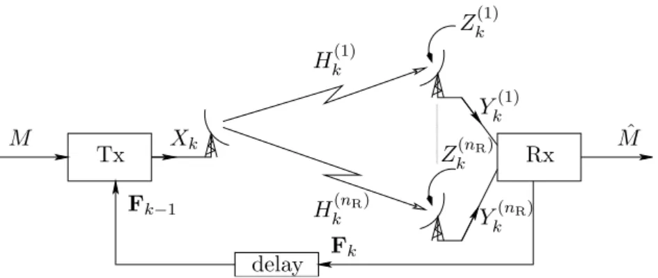
We consider a communication system as shown in Figure 2.1. A message M is transmitted over a SIMO fading channel with memory where the transmitter has one antenna and the receiver has nR antennas. The channel output vector Yk∈ CnR at time k is given by
Yk= Hkxk+ Zk, (2.1)
where xk ∈ C denotes the time-k channel input; the random vector Hk ∈ CnR denotes
the time-k fading vector with nR components corresponding to the nR antennas at the
receiver; and the random vector Zk ∈ CnR models additive noise.
We assume that the additive noise process {Zk} is spatially and temporally
indepen-dent and iindepen-dentically distributed (IID), circularly-symmetric, and complex Gaussian with zero mean and with variance σ2 >0:
{Zk} IID ∼ NC!0, σ2InR
"
. (2.2)
Here, InR denotes the nR× nR identity matrix.
The fading process {Hk} is statistically independent of {Zk} and is assumed to be
stationary, ergodic, of finite energy E#%Hk%2
$
<∞, and of finite differential entropy rate
h({Hk}) > −∞. (2.3)
A random process satisfying this later condition (2.3) is usually called regular. Note that we do not make any further assumptions about {Hk}, i.e., we do not assume a particular law
(like, e.g., a Gaussian distribution). In particular we do allow for arbitrary dependences between the different components%Hk(j)&corresponding to the different antennas (spatial memory) and over time (temporal memory).
We assume noncoherent communication, i.e., neither transmitter nor receiver know the realization of {Hk}, they only know its law.
From the receiver to the transmitter we have a noiseless feedback link (i.e., the link has infinite capacity and allows the receiver to send everything it knows back to the transmitter). However, to preserve causality of the system, we require the feedback to
Chapter 2 Channel Model M Mˆ Tx Rx delay Xk Yk(1) Y(nR) k Hk(1) H(nR) k Zk(1) Z(nR) k Fk Fk−1
Figure 2.1: Regular SIMO fading channel with nR antennas and with noiseless causal
feedback.
be delayed by one discrete time-step. So the feedback vector Fk that is available at the
transmitter at time k consists of all past channel output vectors:
Fk = Y1k−1. (2.4)
The channel input xk at time k therefore is a deterministic function of the message M
and the feedback Y1k−1. Note that we assume M to be uniformly distributed.
We consider two types of power constraints: an average-power constraint and a peak-power constraint. Under the former we require that for every message m
1 n n ' k=1 E())Xk ! m,Yk−11 "))2 * ≤ E, (2.5)
where n denotes the blocklength. Under the peak-power constraint we replace (2.5) with the almost-sure constraint that for every message m
) )Xk
!
m,Y1k−1"))2≤ E, a.s., k = 1, . . . , n. (2.6) To clarify notation we will use a subscript “FB” whenever feedback is available, while the subscript “IID” refers to a situation without memory or feedback. RHS stands for ‘right-hand side’.
Chapter 3
Mathematical Preliminaries
In this chapter, we show some mathematical tools that will be used in our proof.
3.1
Differential Entropy
3.1.1 h+(X)
The differntial entropy h(X) of an n-dimensional real random vector X is defined if the density px(x) (with respect to the Lebesque measure on Rn) is defined and if at least one
of the integrals h+(X)! + {x∈Rn :0<px(x)<1} px(x) log 1 px(x) dx (3.1) h−(X)! + {x∈Rn :px(x)>1} px(x) log px(x) dx (3.2)
is finite. In this case, h(X) is defined as the difference between the two nonnegative integrals,
h(X)! h+(X) − h−(X) (3.3)
where we use the rules +∞ − a = +∞ and a − ∞ = −∞ for all a ∈ R. This is written as h(X) = + Rn px(x) log 1 px(x) dx. (3.4)
The differential entropy of an n-dimensional complex random variable is defined as the differential entropy of the 2n-dimensional real vector comprising of the real and imaginary parts of each of its components. Finally, the differential entropy h(H) of a random matrix His the differential entropy of the vector comprising of its entries.
3.1.2 hλ(·)
Let ˆXk denote the unit vector
ˆ Xk!
Xk
%Xk%
Chapter 3 Mathematical Preliminaries
Because the unit vectors ˆXk only take value on the unit sphere in CnR and since the
surface of this unit sphere has zero measure over CnR, we define a differential entropy-like
quantity hλ(·) that only lives on the surface of the unit sphere in CnR: for V ∈ CnR and
ˆ V! V %V%, we define hλ( ˆV)! E # −log pλ ˆ V( ˆV) $ = − + pλVˆ(ˆv) log pλVˆ(ˆv)dˆv, (3.6) if the expectation exists. Here pλVˆ(ˆv) denotes the PDF of the random unit-vector ˆV with respect to the CnR-surface measure λ. Note that pλ
ˆ
V(ˆv) is implicitly defined by the PDF
of V, pλ
V(v). For more details we refer to [9, Sec. II].
Lemma 3.1 Let V be a complex random vector taking value in Cm and of differntial
entropy h(V). Then
h(V) = h(%V%) + hλ( ˆV|%V%) + (2m − 1)E[log %V%] (3.7)
whenever all the quantities in (3.7) are defined. Here the first term on the right is the differential entropy of %V% when viewed as a real (scalar) random variable.
Note that it is a conditional version of hλ.
3.1.3 Differential Entropy and Expectation of Logarithms
Lemma 3.2 Let X be an n-dimensional complex random vector of density pX(x). Then
the following relationship between differential entropy and the expected log-norm hold: If h−(X) < ∞, then for any 0 < α < n there exists some finite number ∆(n, α) (not depending on the law of X) such that
E[log %X%] ≥ −1 αh
−!X"− ∆(n, α) (3.8)
Proof: See [10, Appendix. A.4.4].
3.2
Markov’s Inequality
Lemma 3.3 (Markov’s Inequality) For any non-negative random variable V and any constant δ > 0,
Pr[V ≥ δ] ≤ E[V ]
δ (3.9)
3.3 Causal Interpretation Chapter 3
3.3
Causal Interpretation
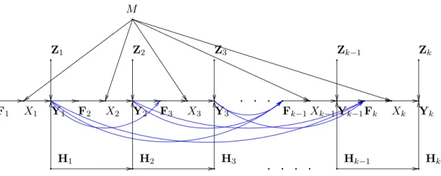
Massey [12], [13] shows a way of graphically determining independence of random variables based on causal interpretations. A causal interpretation is an ordered list of random variables. The idea behind a specific choice of order lies in the causality of the system. Loosely speaking in an engineering way of thinking, we would like to think of some random variables being generated ”first” and some ”later based on” the generation of the others. Note that a priori every ordered list is a valid causal interpretation, but some choices will be more useful keeping the engineering idea in mind.
As an example consider the vector
V = (M, X1k,Y1k,H1k,Zk1,Fk1), (3.10) where all components are random variables defined in Chapter 2.
For simplicity assume for the moment that all components take value in discrete al-phabets1. We choose the following causal interpretation:
(M, H1, ...,Hk,Z1, ...,Zk,F1, X1,Y1,F2, X2,Y2, ...,Fk, Xk,Yk). (3.11)
If we consider now the entropy of V and write it as a sum using the chain rule
H(V) ='
j
H!V(j)))V(1), ..., V(j−1)", (3.12) then we see that our choice of a causal interpretation for V simplifies the expression for the entropy significantly:
H(V) = H(M ) + H(H1) + H(H2|H1) + · · · + H(Hk|Hk1)
+ H(Z1) + · · · + H(Zk) + H(F1)
+ H(X1|F1, M) + H(Y1|X1,H1,Z1) + H(F2|Y1)
+ H(X2|F21, M) + H(Y2|X2,H2,Z2) + · · · + H(Fk|Yk−11 )
+ H(Xk|Fk1, M) + H(Yk|Xk,Hk,Zk) (3.13)
Massey calls this a causal-order expansion of H(V). It can easily be depicted graphically in a causality graph, which is a directed graph with an edge from vertex V(j1) to V(j2) if
and only if V(j1) is in the conditioning expression for H!V(j2)))V(1), ..., V(j2−1)". We shall
say that a vertex V(j1) is causally prior to vertex V(j2) if there is a directed path from
V(j1) to V(j2).
In our case the corresponding graph of (3.11) is shown in Figure 3.2.
Note that once we have established the graph, we do not consider the entropy anymore. We only used the entropy in order to be able to invoke the chain rule in establishing the ”dependencies” between the different components.
1
We will drop this assumption soon again, however, here it simplifies notation considerably because we need not worry about differential entropy. In the end, we are not interested in the entropy at all, but in the ”dependencies” between the components.
Chapter 3 Mathematical Preliminaries X1 X2 X3 Xk−1 Xk F1 F2 F3 Fk−1 Fk Z1 Z2 Z3 Zk−1 Zk Y1 Y2 Y3 Yk−1 Yk H1 H2 H3 Hk−1 Hk M
Figure 3.2: The causality graph of our model.
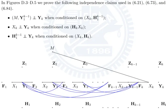
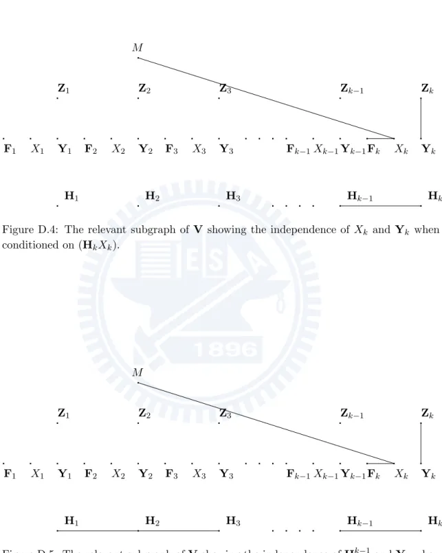
A causality graph is very useful when determining the statistical dependence between two groups of random variables possibly conditioned on a third group.
To state this property in more clarity let A, B, C ⊂ {1, ..., length(V)} be three index sets. Let V(A) denote a vector containing as components of all components of V whose indices are in A, similarly, define V(B) and V(C).
Any causality graph of V can now be used in order to investigate the independence of V(A) and V(B)when conditioned on V(C). To that goal consider the following procedure: • from the specify causality graph take the subgraph causally relevant2 to V(A∪B∪C);
• delete all edges leaving any component of V(C);
• drop all directions of the remaining edges;
• if now all components of V(A) are unconnected to the components of V(B), then V(A) is statistically independent of V(B) when conditioned on V(C).
Note that using this procedure we only make statements about the independence, but not about possible dependences, i.e., if the components of V(A)and V(B)are not disconnected, then they might be statistically dependent or independent.
2
A subgraph causally relevant to some ˜Vconsists of all those vertices that are either components of ˜V or causally prior to ˜Vin the given causal interpretation, together with the edges connecting these vertices.
Chapter 4
Capacity and Fading Number
without Feedback
It has been shown in [8] that the capacity of general regular SIMO fading channels under either an average-power constraint or a peak-power constraint is
C(E) = log(1 + log(1 + E)) + χ({Hk}) + o(1), (4.1)
where o(1) denotes terms that tend to zero as E tends to infinity, and lim
E↑∞{C(E) − log log E} < 0. (4.2)
Therefore, we can define χ({Hk})! lim
E↑∞{C(E) − log log E} (4.3)
= hλ , ˆ H0eiΘ0 ) ) )% ˆH"eiΘ!&−1"=−∞ -− log 2 + nRE#log %H0%2$− h!H0 ) )H−1−∞" (4.4) where the second equality is given by [8] and hλ(·) is defined in 3.1.2. Here, {Θk} is IID
∼ U((−π, π]) and independent of {Hk}.
From (4.1) it is obvious that the capacity of the fading channel (2.1) grows extremely slowly at large power. Indeed, log(1 + log(1 + E)) grows so slowly that, for the smallest values of E for which o(1) ≈ 0, the (constant!) fading number χ usually is much larger than log(1 + log(1 + E)). Hence, the threshold between the low-power regime and the capacity-inefficient high-power regime is strongly related to the fading number: the larger the fading number is, the higher the rate can be chosen without operating the system in the inefficient double-logarithmic regime.
Also note that even though the double-logarithmic term on the RHS of (4.1) does not depend on {Hk} or, particularly, on the number of antennas nR, it is still beneficial to
have multiple antennas because the fading number χ does depend strongly on the fading process and the number of antennas.
Chapter 4 Capacity and Fading Number without Feedback
From (4.4) one also sees that in the case of a memoryless SIMO fading channel, the fading number is given by
χIID(H) = hλ! ˆHeiΘ
"
− log 2 + nRE#log %H%2$− h(H), (4.5)
and that therefore the fading number in (4.4) also can be written as χ({Hk}) = χIID(H0) + I ! H0; H−1−∞ " − I,Hˆ0eiΘ0;% ˆH"eiΘ! &−1 "=−∞ -. (4.6)
In [8], it has also been shown that for an arbitrary value of the power E, the channel capacity can be bounded as follows:
C(E) ≤ CIID(E) + I!H0; H−1−∞", E ≥ 0. (4.7) From (4.6) we see that this upper bound may not be tight. In particular, asymptotically for E → ∞ it is strictly loose.
Chapter 5
Capacity and Fading Number with
Feedback
While it is well-known that feedback has no effect on the capacity of a memoryless channel, in general feedback does increase capacity for channels with memory. The reason for this is that the combination of feedback and memory allows the transmitter to predict the current channel state and thereby adapt to it. Unfortunately, for regular fading channels this increase in capacity due to the feedback turns out to be very limited.
Theorem 5.1 (Capacity Increase by Feedback is Bounded by a Constant) Let a general SIMO fading channel with memory be defined as in (2.1) and consider a noiseless causal feedback link as described in (2.4) (see Figure 2.1). Then the channel capacity under either an average-power constraint (2.5) or a peak-power constraint (2.6) is upper-bounded as follows:
CFB(E) ≤ CIID(E) + I!H0; H−1
−∞
"
, E ≥ 0. (5.1)
Proof: When we defined channel capacity, we relied on a result by Dobrusin [14] which shows that for information stable channels the capacity is given by
C= lim
n→∞
1
nQ∈P(Xsupn)
I(X1n; Y1n), (5.2)
where P(Xn) is the set of all probability measures Q over Xn satisfying the given input
constraints.
Here, however, we have feedback and can therefore not rely on the above result, but have to derive a new converse to the coding theorem for the new situation.
Note that since the channel capacity under a peak-power constraint E cannot be larger than the capacity under an average-power constraint E, all upper bounds that are based on an average-power constraint are also valid for the situation with a peak-power constraint. We will therefore in the following only consider an average-power constraint.
Hence, assume that there is a sequence of code schemes with ,enRFB- codewords of
Chapter 5 Capacity and Fading Number with Feedback
probability of error
Pe(n)! Pr[ ˆM .= M ] (5.3)
tends to zero as n tends to infinity. Then
H(M ) = log,enRFB- ≥ log(enRFB− 1) = nR FB− )n, (5.4) where )n→ 0 as n → ∞. Therefore, RFB ≤ 1 nH(M ) + )n n (5.5) = 1 nI(M ; Y n 1) + 1 nH(M |Y n 1) + )n n (5.6) = 1 nI(M ; Y n 1) + log 2 + Pe(n)log,enRFB -n + )n n (5.7) = 1 nI(M ; Y n 1) + log 2 n + Pe(n)nRFB n + )n n (5.8) = 1 nI(M ; Y n 1) + log 2 n + P (n) e RFB+ )n n (5.9)
Here (5.6) follows from that definition of mutual information, and the subsequent inequal-ity from Fano’s inequalinequal-ity.
Therefore, for n → ∞ we must have RFB ≤ lim n→∞ 1 nI(M ; Y n 1). (5.10)
Hence, any upper bound on the RHS of (5.10) will yield an upper bound on channel capacity in presence of feedback. We will therefore continue with bounding I(M ; Yn
1): 1 nI(M ; Y n 1) = 1 n n ' k=1 I(M ; Yk|Yk−11 ) (5.11) = 1 n n ' k=1 , I(M, Y1k−1; Yk) − I(Y1k−1; Yk) -(5.12) ≤ 1 n n ' k=1 I(M, Yk−11 ; Yk) (5.13) ≤ 1 n n ' k=1 I(M, Yk−11 ,Hk−11 ; Yk) (5.14) = 1 n n ' k=1 I(M, Yk−11 ,Hk−11 , Xk; Yk) (5.15) = 1 n n ' k=1 , I(Hk−11 , Xk; Yk) + I(M, Yk−11 ; Yk|Hk−11 , Xk) -(5.16) = 1 n n ' k=1 I(Hk−11 , Xk; Yk) (5.17) = 1 n n ' k=1 , I(Xk; Yk) + I(Hk−11 ,Yk|Xk) -. (5.18)
Chapter 5
Here the first two equalities follow from the chain rule; the subsequent inequality from the non-negativity of mutual information; the following inequality from adding more terms; the subsequent equality follows since Xk is a deterministic function of M and Y1k−1 (and
hypothetically also Hk−11 ); then we have used the chain rule again; (5.17) follows since3
I(M, Yk−11 ; Yk|Hk−11 , Xk) = 0 (5.19)
and finally we have used the chain rule once more.
We have to take into account that Xk depends on past outputs via the feedback in the
next step. I(Hk−11 ; Yk|Xk) ≤ I(H1k−1; Yk,Hk|Xk) (5.20) = I(Hk−11 ; Hk|Xk) + I(H1k−1; Yk|Xk,Hk) (5.21) = I(Hk−11 ; Hk|Xk) (5.22) = h(Hk|Xk) − h(Hk|Hk−11 , Xk) (5.23) ≤ h(Hk) − h(Hk|Hk−11 , Xk) (5.24) = h(Hk) − h(Hk|Hk−11 ) (5.25) = I(Hk; Hk−11 ) (5.26)
Here the first inequality follows from adding one more term; the subsequent equality follows from the chain rule; (5.22) follows since
I(Hk−11 ; Yk|Xk,Hk) = 0 (5.27)
which can be seen similarly to (5.19); (5.24) is due to conditioning that reduces entropy; and the subsequent equality holds since conditional on Hk−11 , Xkand Hkare independent.
Together with (5.18) this yields 1 nI(M ; Y n 1) ≤ 1 n n ' k=1 , I(Xk; Yk) + I(Hk; Hk−11 ) -(5.28) ≤ 1 n n ' k=1 , I(Xk; Yk) + I(Hk; Hk−1−∞) -(5.29) ≤ 1 n n ' k=1 CIID(Ek) + I(H0; H−1−∞) (5.30)
where in the last inequality we have used the stationarity of {Hk} and used CIID(Ek) to
denote the capacity without feedback or memory for a given power Ek. Note that the
3
To see this keep in mind that Ykis fully determined by Zk, Hk, and Xk. The noise Zkis independent
of everything else and can therefore not be estimated from any other random variable; Xk is given; only
Hkis not known. However, it can be approximated using the past H k
−1
1 which again are given. Therefore,
conditional on Hk−1
1 and Xk, M and Y k
−1
1 are independent of Yk. This statement can also be proven
Chapter 5 Capacity and Fading Number with Feedback
power allocation depends on the feedback. However, due to (2.5) Ek must satisfy
1 n n ' k=1 Ek ≤ E. (5.31)
Using this together with Jensen’s inequality relying on the concavity of channel capacity in the power, we get
1 nI(M ; Y n 1) ≤ CIID . 1 n n ' k=1 Ek / + I(H0; H−1−∞) (5.32)
≤ CIID(E) + I(H0; H−1−∞) (5.33)
where in the second inequality we used the fact that CIID(·) is nondecreasing.
Therefore, RFB(E) ≤ lim n→∞ 1 nI(M ; Y n
1) ≤ CIID(E) + I(H0; H−1−∞) (5.34)
which proves (5.1).
We note that the RHS of (5.1) is identical to the RHS of (4.7). Hence the same (alas potentially loose) bound holds both for the channel capacity with and without feedback. Moreover, also note that C(E) trivially is a lower bound to CFB(E) since the transmitter
can simply ignore the feedback and achieve the same results as without feedback.
An immediate consequence of Theorem 5.1 is that CFB(E) only grows
double-logarith-mically in the power at high power and therefore there exists a fading number χFB({Hk})
with a definition as follows: Corollary 5.2 Because
lim
E↑∞{CFB(E) − log log E} < 0, (5.35)
we define
χFB({Hk})! lim
E↑∞{CFB(E) − log log E} (5.36)
(5.37) Theorem 5.1 can then be applied to χFB({Hk}).
Corollary 5.3 Using the same result as in Theorem 5.1, we learn χFB({Hk}) ≤ χIID({Hk}) + I
!
H0; H−1−∞
"
. (5.38)
Chapter 5
Theorem 5.4 (SIMO Fading Number with Feedback) Let a general SIMO fading channel with memory be defined as in (2.1) and consider a noiseless causal feedback link as described in (2.4) (see Figure 2.1). Then the asymptotic channel capacity under either an average-power constraint (2.5) or a peak-power constraint (2.6) is identical to the asymptotic channel capacity for the channel without feedback: CFB(E) = log(1 + log(1 + E)) + χFB({Hk}) + o(1) (5.39) where the fading number is
χFB({Hk}) = χ({Hk}) = hλ , ˆ H0eiΘ0 ) ) )% ˆH"eiΘ! &−1 "=−∞ -− log 2 + nRE#log %H0%2$− h!H0 ) )H−1−∞". (5.40)
We would like to point out that this result even holds in the (hypothetical) case when the feedback is improved in the sense that in addition to the past channel outputs the transmitter also is informed about the past fading realizations Hk−11 . Note further that since we have assumed the most optimistic form of causal feedback, any type of realistic feedback will yield the same result.
We would like to give a hand-waving explanation of this behavior. Since the fading process is assumed to be regular with a finite differential entropy rate, it is not possible to perfectly predict the future realizations of the process even if one is presented with the exact realizations of the infinite past. Nevertheless, the feedback allows the transmitter to make an estimate of future realizations. Based on these estimates, the transmitter can then perform elaborate schemes of optimal power allocation over time: if the channel state is likely to be poor, it saves power and uses it once the channel state is likely to be good again. Unfortunately, due to the double-logarithmic behavior of capacity, such power allocation has no effect at all as can be seen as follows: for any constant β > 0 (β can be chosen arbitrarily large!),
lim
E↑∞{log log βE − log log E} = limE↑∞{log(log β + log E) − log log E} (5.41)
= lim
E↑∞{log(log E) − log log E} (5.42)
= 0. (5.43)
So not only the double-logarithmic growth is left untouched, but also the second term, i.e., the fading number, remains unchanged.
Chapter 6
Proof of Theorem 5.4
6.1
Main Line Through the Proof
Since the channel capacity of the system without feedback trivially is a lower bound on the channel capacity with feedback, and since the capacity under a peak-power constraint is a lower bound on the capacity with an average-power constraint, it is sufficient to derive an upper bound on χFB({Hk}) under the assumption of the average-power constraint (2.5)
and to show that it is identical to the fading number without feedback and under the assumption of a peak-power constraint.
The proof is very lengthy and we therefore outline the main ideas in the beginning. The basic structure follows the proof of the general fading number of MIMO fading channels with memory given in [9]. However, there are many details that need to be adapted and taken care of. Particularly, we have to consider the following challenges:
• Due to the feedback, the channel input, the fading, and the additive noise become dependent.
• We cannot rely on the important auxiliary result given in [9, Th. 3] that shows that the optimal input is stationary.
• We cannot rely on the important auxiliary result given in [15, Th. 8] that shows that the capacity-achieving input distribution escapes to infinity.
To handle the first challenge, we often rely on the concept of causal interpretations, which is introduced in Chapter 3.3, [12], [13]. This is a tool that allows to graphically proof the independence of random variables when conditioned on certain other random variables.
The missing auxiliary result concerning the capacity-achieving input distribution es-caping to infinity can be proven indirectly inside of the derivation.
The biggest difficulty is caused by the nonstationarity of the channel input that is inherent to the given context because the transmitter continuously learns more about the fading process through the feedback and thereby changes the optimal distribution of the input.
6.1 Main Line Through the Proof Chapter 6
The proof starts with Fano’s inequality (see (5.9)), which states that any given sequence of communication systems with rate RFB and power E must satisfy
RFB(E) ≤ 1 nI ! M; Y1n"+log 2 n + P (n) e RFB(E) + )n n (6.1) = 1 n n ' k=1 I!M; Yk ) )Yk−11 "+log 2 n + P (n) e RFB(E) + )n n (6.2) = 1 n κ ' k=1 I!M; Yk ) )Yk−11 "+n− κ n− κ 1 n n ' k=κ+1 I!M; Yk ) )Y1k−1" +log 2 n + P (n) e RFB(E) + )n n (6.3) ≤ 1 n κ ' k=1 , CIID(Ek) + I!H0; H−1−∞"-+n− κ n 1 n− κ n ' k=κ+1 I!M; Yk ) )Yk−11 " +log 2 n + P (n) e RFB(E) + )n n (6.4)
In (6.3), we separate the sum into two parts. The first part, 1 ≤ k ≤ κ, can be considered as transient state. Since κ is a constant, it is bounded anyway and in (6.4) we bound the mutual information term in the sum as in (5.30). Using Jensen’s inequality relying on the concavity of channel capacity in the power, we get
RFB(E) ≤ κ nCIID . 1 κ κ ' k=1 Ek / +κ nI ! H0; H−1−∞ " +n− κ n 1 n− κ n ' k=κ+1 I!M; Yk ) )Y1k−1" +log 2 n + P (n) e RFB(E) + )n n. (6.5)
Next we focus on κ + 1 ≤ k ≤ n and bound as follows: I!M; Yk ) )Yk−11 "≤ I!M; Yk, Gk ) )Yk−11 " (6.6) = I!M; Gk ) )Yk−11 "+ I!M; Yk ) )Y1k−1, Gk " (6.7) = H!Gk ) )Y1k−1"− H!Gk ) )M, Y1k−1" 0 12 3 ≥ 0 + γkI ! M; Yk ) )Y1k−1, Gk= 1 " + (1 − γk)I ! M; Yk ) )Yk−11 , Gk= 0 " . (6.8)
Here in (6.6), we add the indicator random variable Gk that is defined as
Gk !
4
1 if %Hk%2 ≥ t,
0 otherwise, (6.9)
for some given t > 0. We will choose t large such that E#%H0%2 $ t ≤ 0.5 (6.10) Moreover, we define γk! Pr[Gk = 1] = Pr # %Hk%2≥ t $ , (6.11)
Chapter 6 Proof of Theorem 5.4
and note that by the Markov inequality (Lemma 3.3), γk= Pr # %Hk%2≥ t $ ≤ E # %Hk%2 $ t . (6.12) Because H!Gk ) )Y1k−1"≤ H(Gk) = Hb(γk) ≤ Hb . E#%Hk%2 $ t / (6.13) where Hb(·) denoting the binary entropy function, with t large enough and by using (5.30)
again with conditioning on Gk= 1, we further bound (6.8) as follows:
I!M; Yk ) )Yk−11 " ≤ Hb(γk) + γkCIID(Ek ) )Gk= 1) + γkI ! H0; H−1−∞ ) )G0= 1 " + (1 − γk) 0 12 3 ≤1 I!M; Yk ) )Y1k−1, Gk= 0 " (6.14) ≤ Hb . E#%H0%2$ t / +E # %H0%2$ t C˜IID(tEk) + E#%H0%2$ t I ! H0; H−1−∞ ) )G0 = 1" + I!M; Yk ) )Yk−11 , Gk = 0 " . (6.15)
Here in (6.15), ˜CIID(·) is the capacity of a channel ˜ Yk = Yk t = Hk t xk+ Zk t ! ˜Hkxk+ ˜Zk (6.16)
where we condition on the event that Gk = 1, i.e., %Hk%2 > t. This is a different regular
fading channel, for which we know lim
˜ E→∞
{ ˜CIID( ˜E) − log log ˜E} ≤ ∞. (6.17)
Hence, 1 n n ' k=κ+1 ˜ CIID(t · Ek) ≤ 1 n n ' k=1 ˜ CIID(t · Ek) ≤ ˜CIID . t· 1 n n ' k=1 Ek /
where the last inequality follows by Jensen’s inequality relying on the concavity of channel capacity in the power again. Putting everything back into (6.5), we get
RFB(E) ≤ κ nCIID . 1 κ κ ' k=1 Ek / +κ nI ! H0; H−1−∞ " +n− κ n 1 n− κ n ' k=κ+1 I!M; Yk ) )Yk−11 , Gk= 0 " +n− κ n Hb . E#%H0%2 $ t / +E # %H0%2 $ t C˜IID . t· 1 n n ' k=1 Ek / +n− κ n E#%H0%2 $ t I ! H0; H−1−∞ ) )G0= 1 " +log 2 n + P (n) e RFB(E) + )n n. (6.18)
6.1 Main Line Through the Proof Chapter 6
The third term in (6.18) is then bounded as follows: I!M; Yk ) )Y1k−1, Gk= 0 " = I!M,Y1k−1; Yk ) )Gk= 0 " − I!Y1k−1; Yk ) )Gk= 0 " (6.19) ≤ I!M,Y1k−1, Xk,Hk−11 ; Yk ) )Gk = 0 " − I!Yk−11 ; Yk ) )Gk= 0 " (6.20) = I!Xk,Hk−11 ; Yk ) )Gk= 0 " + I!M,Yk−11 ; Yk ) )Xk,Hk−11 , Gk= 0 " 0 12 3 = 0, see Appendix D − I!Y1k−1; Yk ) )Gk = 0 " (6.21) ≤ I!Ek, Xk,Hk−11 ; Yk ) )Gk= 0 " − I!Yk−11 ; Yk ) )Gk= 0 " (6.22) = I(Ek; Yk ) )Gk= 0) + I(Xk; Yk|Ek, Gk= 0) + I!Hk−11 ; Yk ) )Xk, Ek, Gk= 0 " − I!Y1k−1; Yk ) )Gk= 0 " (6.23) ≤ Hb(βk) + βkI(Xk; Yk|Ek= 1, Gk= 0) + βkI ! Hk−11 ; Yk ) )Xk, Ek= 1, Gk= 0 " − I!Y1k−1; Yk, Gk= 0 " + (1 − βk)I ! Xk,Hk−11 ; Yk ) )Ek= 0, Gk= 0 " . (6.24)
Here in (6.20) the current input Xkand the past fading values Hk−11 are added. In (6.22)
we add the indicator random variable Ek that is defined as
Ek!
4
1 if |X"| ≥ ξmin, ∀ , = 1, . . . , k,
0 otherwise, (6.25)
for some given ξmin ≥ 0. Moreover, βk ! Pr [Ek= 1|Gk= 0]. Finally, (6.24) follows
because we bound I(Ek; Yk ) )Gk= 0) = H(Ek ) )Gk= 0) − H(Ek|Yk, Gk= 0) 0 12 3 ≥ 0 ≤ H(Ek) = Hb(βk). (6.26)
Note that the three middle terms on the RHS of (6.24) correspond to a memoryless term, a term with memory, and a correction term, respectively. We will show in Section 6.2 that the second term on the RHS of (6.24) can be bounded as follows:
I(Xk; Yk|Ek= 1, Gk= 0) = hλ , ˆ HkeiΘk ) ) )Ek = 1, Gk= 0 -− h(Hk ) )Xk, Ek= 1, Gk= 0) − log 2 + nRE#log %Hk%2 ) )Ek= 1, Gk= 0 $ + µ,log η − E#log %Hk%2 ) )Ek= 1, Gk= 0 $ − E#log |Xk|2 ) )Ek= 1, Gk = 0 $ -+ log Γ 5 µ,ν η 6 + )ν,k+ 1 ηE # %H2k%|Xk|2 ) )Ek= 1, Gk= 0 $ +ν η, (6.27)
the third term on the right hand side of (6.24) as I!Hk−11 ; Yk ) )Xk, Ek= 1, Gk= 0 " ≤ h(Hk ) )Xk, Ek= 1, Gk = 0) − h ! Hk ) )Hk−11 , Gk= 0 " , (6.28)
Chapter 6 Proof of Theorem 5.4
and the fourth term on the right hand side of (6.24) as I!Yk−11 ; Yk ) )Gk = 0 " ≥ βkhλ! ˆHkeiΘk ) )Ek= 1, Gk = 0 " − hλ 5 ˆ HkeiΘk ) ) ) ) 7 ˆ HleiΘl 8k−1 l=k−κ, Gk= 0 6 + (1 − βk)hλ 5 ˆ HkeiΘk ) ) ) ) 7 ˆ HleiΘl 8k−1 k−κ, Ek= 0, Gk= 0 6 − 3Hb(βk) − δ1(κ, ξmin) − δ2(κ, ξmin). (6.29)
Plugging (6.27), (6.28), and (6.29) back to (6.24), we get I!M; Yk ) )Yk−11 , Gk= 0 " ≤ Hb(βk) + βkhλ! ˆHkeiΘk|Ek= 1, Gk= 0"− βkh(Hk|Xk, Ek= 1, Gk= 0) − βklog 2 + βknRE # log %Hk%2 ) )Ek= 1, Gk= 0 $ + βkµ , log η − E#log %Hk%2 ) )Ek = 1, Gk= 0 $ − E#log |Xk|2|Ek= 1, Gk= 0 $ -+ βklog Γ 5 µ,ν η 6 + βk)ν,k+ βk 1 ηE # %H2k%|Xk|2 ) )Ek= 1, Gk = 0 $ + βk ν η + βkh(Hk|Xk, Ek= 1, Gk= 0) − βkh!Hk ) )Hk−11 , Gk = 0" − βkhλ! ˆHkeiΘk ) )Ek= 1, Gk= 0 " + hλ 5 ˆ HkeiΘk ) ) ) ) 7 ˆ HleiΘl 8k−1 l=k−κ, Gk= 0 6 − (1 − βk)hλ 5 ˆ HkeiΘk ) ) ) ) 7 ˆ HleiΘl 8k−1 l=k−κ, Ek= 0, Gk = 0 6 + 3Hb(βk) + δ1(κ, ξmin) + δ2(κ, ξmin) + (1 − βk)I ! Xk,Hk−11 ; Yk ) )Ek = 0, Gk = 0 " . (6.30)
Note that the four underlining terms in (6.30) cancel each other, and that βknRE#log %Hk%2 ) )Ek = 1, Gk= 0 $ = nRE#log %Hk%2 ) )Gk = 0 $ − (1 − βk)nRE#log %Hk%2 ) )Ek = 0, Gk= 0 $ , −µβkE # log %Hk%2 ) )Ek= 1, Gk= 0 $ = −µE#log %Hk%2 ) )Gk= 0 $ + µ(1 − βk)E # log %Hk%2 ) )Ek= 0, Gk= 0 $ . Moreover, E#log |Xk|2|Ek= 1, Gk= 0 $ ≥ log ξmin2 , and by (B.10) and (B.11) βk)ν,k = sup γ≥ξmin 7 βkE#log(%Hk%2γ2+ ν) ) )Ek= 1, Gk= 0$ − βkE # log(%Hk%2γ2) ) )Ek= 1, Gk= 0 $ 8 (6.31) ≤ sup γ≥ξmin 7 βkE # log(%Hk%2γ2+ ν) ) )Ek= 1, Gk= 0 $ − βkE # log(%Hk%2γ2) ) )Ek= 1, Gk= 0 $
6.1 Main Line Through the Proof Chapter 6 + (1 − βk)E # log(%Hk%2γ2+ ν) ) )Ek= 0, Gk= 0 $ − (1 − βk)E # log(%Hk%2γ2) ) )Ek= 0, Gk= 0 $ 8 = sup γ≥ξmin % E#log(%H0%2γ2+ ν) ) )Gk= 0 $ − E#log(%H0%2γ2) ) )Gk = 0 $& (6.32) = )ν (6.33)
where (6.32) follows because we add something positive (ν ≥ 0, chosen freely). Therefore, (6.30) becomes I!M; Yk ) )Y1k−1, Gk= 0 " ≤ Hb(βk) − βklog 2 + nRE # log %Hk%2 ) )Gk= 0 $ − (1 − βk) nRE#log %Hk%2 ) )Ek= 0, Gk= 0 $ + βkµlog η − µE # log %Hk%2 ) )Gk= 0 $ + µ(1 − βk)E # log %Hk%2 ) )Ek= 0, Gk = 0 $ − βkµlog ξmin2 + βklog Γ 5 µ,ν η 6 + )ν + βk 1 ηE # %H2k%|Xk|2 ) )Ek = 1, Gk= 0 $ + βk ν η − βkh ! Hk ) )Hk−11 , Gk= 0 " + hλ 5 ˆ HkeiΘk ) ) ) ) 7 ˆ HleiΘl 8k−1 l=k−κ, Gk= 0 6 − (1 − βk)hλ 5 ˆ HkeiΘk ) ) ) ) 7 ˆ HleiΘl 8k−1 l=k−κ, Ek= 0, Gk= 0 6 + 3Hb(βk) + δ1(κ, ξmin) + δ2(κ, ξmin) + (1 − βk)I!Xk,Hk−11 ; Yk ) )Ek= 0, Gk= 0" (6.34) = 4Hb(βk) + δ1(κ, ξmin) + δ2(κ, ξmin) + )ν + hλ 5 ˆ HkeiΘk ) ) ) ) 7 ˆ HleiΘl 8k−1 l=k−κ, Gk= 0 6 − βkh ! Hk ) )Hk−11 , Gk= 0 " + nRE#log %Hk%2 ) )Gk= 0 $ + µ,βklog η − E # log %Hk%2 ) )Gk = 0 $ + (1 − βk)E # log %Hk%2 ) )Ek= 0, Gk= 0 $ − βklog ξ2min -+ βklog Γ 5 µ,ν η 6 +βk η E # %Hk%2|Xk|2|Ek = 1, Gk= 0 $ + βk ν η − βklog 2 + (1 − βk) . I!Xk,Hk−11 ; Yk ) )Ek= 0, Gk= 0 " − hλ 5 ˆ HkeiΘk ) ) ) ) 7 ˆ HleiΘl 8k−1 l=k−κ, Ek = 0, Gk= 0 6 − nRE#log %Hk%2 ) )Ek= 0, Gk= 0 $ / . (6.35)
Here, in (6.35) we arithmetically rearrange the terms. We further bound the last term in (6.35) as follows: (1 − βk)E # log %Hk%2 ) )Ek= 0, Gk= 0 $ ≤ (1 − βk) log E # %Hk%2 ) )Ek= 0, Gk= 0 $ (6.36)
Chapter 6 Proof of Theorem 5.4 ≤ (1 − βk) log E#%Hk%2 ) )Gk = 0$ (1 − βk) (6.37) = (1 − βk) log E # %H0%2 ) )G0 = 0$− (1 − βk) log(1 − βk) (6.38) ≤ (1 − βk) log E # %H0%2 ) )G0 = 0$− e−1log e−1 (6.39) = (1 − βk) log E # %H0%2 ) )G0 = 0$+ 1 e, (6.40)
where (6.36) follows from Jensen’s inequality; (6.37) follows because E#%Hk%2 ) )Gk= 0 $ = βkE # %Hk%2 ) )Ek= 1, Gk= 0 $ + (1 − βk)E # %Hk%2 ) )Ek= 0, Gk= 0 $ (6.41) ≥ (1 − βk)E # %Hk%2 ) )Ek= 0, Gk= 0 $ ; (6.42)
(6.38) follows because {Hk} is a stationary process; and (6.39) follows because the function
x 0→ x log x has its minimum when x = e. Putting (6.40) back into (6.35) and using the stationarity property of {Hk} again, we get
I!M; Yk ) )Yk−11 , Gk= 0 " ≤ 4Hb(βk) + δ1(κ, ξmin) + δ2(κ, ξmin) + )ν + hλ! ˆH0eiΘ0 ) ){ ˆHleiΘl }−1l=−κ, G0 = 0"− βkh ! H0 ) )H−1−k+1, G0 = 0" + nRE # log %H0%2 ) )G0= 0$ + µ,βklog η − E # log %H0%2 ) )G0 = 0 $ + (1 − βk) log E # %H0%2))G0 = 0$+1 e − βklog ξ 2 min -+ βklog Γ 5 µ,ν η 6 +βk η E # %Hk%2|Xk|2 ) )Ek= 1, Gk= 0 $ + βk ν η − βklog 2 + (1 − βk) . I!Xk,Hk−11 ; Yk ) )Ek = 0, Gk= 0 " − hλ 5 ˆ HkeiΘk ) ) ) ) 7 ˆ HleiΘl 8k−1 l=k−κ, Ek= 0, Gk= 0 6 − nRE#log %Hk%2 ) )Ek = 0, Gk = 0 $ / . (6.43)
Next note that βk η E # %Hk%2|Xk|2 ) )Ek= 1, Gk= 0 $ = 1 ηE # %Hk%2|Xk|2 ) )Gk= 0 $ −1 − βk η E # %Hk%2|Xk|2 ) )Ek= 0, Gk= 0 $ (6.44) ≤ 1 ηE # %Hk%2|Xk|2 ) )Gk= 0 $ . (6.45)
6.1 Main Line Through the Proof Chapter 6
Moreover in Appendix A, we further bound the last part of (6.43) as follows: I!Xk,Hk−11 ; Yk ) )Ek= 0, Gk = 0 " − hλ 5 ˆ HkeiΘk ) ) ) ) 7 ˆ HleiΘl 8k−1 l=k−κ, Ek= 0, Gk = 0 6 −nRE#log %Hk%2 ) )Ek= 0, Gk= 0 $ ≤ CIID(ξmin ) )Gk= 0) − (nR− 1)h(H0 ) )H−1−∞, G0 = 0) − hλ! ˆH0eiΘ0))H−1−∞, G0 = 0"− h(H0))H−1−k+1, G0= 0) +nR(nR+ 1) e + n 2 Rlog+ . πe nR E#%H0%2|G0 = 0$ 1 − βk / + nR∆(nR,1). (6.46) where
log+(x)! max{0, log(x)} (6.47)
and ∆(nR,1) is some finite number. Therefore, we get
I!M; Yk ) )Y1k−1, Gk= 0" ≤ 4Hb(βk) + δ1(κ, ξmin) + δ2(κ, ξmin) + )ν + hλ! ˆH0eiΘ0)){ ˆHleiΘl}−1l=−κ, G0 = 0"− βkh ! H0))H−1−k+1, G0 = 0" + nRE#log %H0%2 ) )G0 = 0$ + µ,βklog η − E # log %H0%2 ) )G0 = 0$ + (1 − βk) log E # %H0%2 ) )G0= 0$+ 1 e− βklog ξ 2 min -+ βklog Γ 5 µ,ν η 6 + 1 ηE # %Hk%2|Xk|2 ) )Gk= 0 $ + βk ν η − βklog 2 + (1 − βk) . CIID(ξmin ) )Gk = 0) − (nR− 1)h(H0 ) )H−1−∞, G0= 0) − hλ! ˆH0eiΘ0 ) )H−1−∞, Gk= 0 " − h(H0 ) )H−1−k+1, G0 = 0) +nR(nR+ 1) e + n 2 Rlog+ . πe nR E#%H0%2|G0 = 0$ 1 − βk / + nR∆(nR,1) / (6.48) ≤ 4Hb(βk) + δ1(κ, ξmin) + δ2(κ, ξmin) + )ν + hλ! ˆH0eiΘ0 ) ){ ˆHleiΘl}l=−κ−1 , G0 = 0"− h!H0 ) )H−1−∞, G0 = 0" + nRE#log %H0%2 ) )G0 = 0$ + µ,βklog η − E # log %H0%2 ) )G0 = 0$ + (1 − βk) log E # %H0%2 ) )G0= 0$+ 1 e− βklog ξ 2 min -+ βklog Γ 5 µ,ν η 6 + 1 ηE # %Hk%2|Xk|2 ) )Gk= 0 $ + βk ν η − βklog 2 + (1 − βk) . CIID(ξmin ) )Gk = 0) − (nR− 1)h(H0 ) )H−1−∞, G0= 0)
Chapter 6 Proof of Theorem 5.4 − hλ! ˆH0eiΘ0 ) )H−1−∞, Gk= 0 " +nR(nR+ 1) e + n 2 Rlog+ . πe nR E#%H0%2|G0 = 0$ 1 − βk / + nR∆(nR,1) / , (6.49) where (6.49) follows because two underlining terms in (6.48) combine to
h!H0 ) )H−1−k+1, G0 = 0). Defining β ! 1 n− κ n ' k=κ+1 βk, (6.50)
using Jensen’s inequality for the binary entropy function, adding the sum from (6.18) in front of (6.49), we get 1 n− κ n ' k=κ+1 I!M; Yk ) )Yk−11 , Gk = 0 "
≤ 4Hb(β) + δ1(κ, ξmin) + δ2(κ, ξmin) + )ν+ hλ! ˆH0eiΘ0
) ){ ˆHleiΘl }−1l=−κ, G0= 0" − h!H0 ) )H−1−∞, G0= 0"+ nRE#log %H0%2, G0= 0$ + µ!βlog η − E#log %H0%2 ) )G0= 0$+ (1 − β) log E#log %H0%2 ) )G0 = 0$ +1 e− β log ξ 2 min " + β log Γ 5 µ,ν η 6 + 1 η 1 n− κ n ' k=κ+1 E#%Hk%2|Xk|2 ) )Gk= 0 $ + βν η − β log 2 + (1 − β),CIID(ξmin ) )G0 = 0"− (nR− 1)h ! H0 ) )H−1−∞, G0 = 0" − hλ( ˆH0eiΘ0 ) )H−1−∞, G0 = 0) + nR(nR+ 1) e + nR∆(nR,1) -+ 1 n− κ n ' k=κ+1 (1 − βk)n2Rlog+ . πe nR E#%H0%2 ) )G0 = 0$ 1 − βk / . (6.51)
Because for βk ≥ 1 −πeE[
%H0%2|G0=0] nR , (1 − βk) log + . πe nR E!%H0%2 ) )G0=0 " 1−βk / is concave in βk,
the last term in (6.51) can be further bounded as 1 n− κ n ' k=κ+1 (1 − βk)n2Rlog+ . πe nR E#%H0%2 ) )G0= 0$ 1 − βk / ≤ (1 − β)n2Rlog+ . πe nR E#%H0%2))G0 = 0$ 1 − β / . (6.52)
6.1 Main Line Through the Proof Chapter 6
on {Xk}), we add a supremum over β:
1 n− κ n ' k=κ+1 I!M; Yk ) )Yk−11 , Gk = 0 " ≤ hλ! ˆH0eiΘ0 ) ){ ˆHleiΘl}−1l=−κ, G0 = 0 " − h!H0 ) )H−1−∞, G0 = 0" − log 2 + nRE#log %H0%2))G0= 0$ + sup 0≤β≤1 4 4Hb(β) + δ1(κ, ξmin) + δ2(κ, ξmin) + )ν + µ!βlog η − E#log %H0%2 ) )G0= 0 $ + (1 − β) log E#log %H0%2 ) )G0 = 0 $ + e−1− β log ξmin2 " + β log Γ 5 µ,ν η 6 + 1 η 1 n− κ n ' k=κ+1 E#%Hk%2|Xk|2 ) )Gk= 0 $ + βν η + (1 − β),CIID(ξmin ) )G0 = 0) − (nR− 1)h!H0 ) )H−1−∞, Gk= 0 " + log 2 − hλ( ˆH0eiΘ0 ) )H−1−∞, G0 = 0) +nR(nR+ 1) e + nR∆(nR,1) -+ (1 − β)n2Rlog+ . πe nR E[%H0%2 ) )G0= 0] 1 − β / 9 . (6.53) Because 1 ηE # %Hk%2|Xk|2 ) )Gk = 0 $ ≤ 1 ηE # t· |Xk|2 ) )Gk= 0 $ ≤ t ηEk (6.54) and t η 1 n− κ n ' k=κ+1 Ek ≤ t η n n− κ 1 n n ' k=1 Ek 0 12 3 ≤ E ≤ t η n n− κE, (6.55) (6.53) becomes 1 n− κ n ' k=κ+1 I!M; Yk ) )Yk−11 , Gk = 0 " ≤ hλ! ˆH0eiΘ0 ) ){ ˆHleiΘl}−1 l=−κ, G0 = 0 " − h!H0 ) )H−1−∞, G0 = 0" − log 2 + nRE#log %H0%2 ) )G0= 0$ + sup 0≤β≤1 4 4Hb(β) + δ1(κ, ξmin) + δ2(κ, ξmin) + )ν + µ!βlog η − E#log %H0%2 ) )G0= 0$+ (1 − β) log E#log %H0%2 ) )G0 = 0$ + e−1− β log ξmin2 " + β log Γ 5 µ,ν η 6 + t η n n− κE + β ν η + (1 − β),CIID(ξmin ) )G0 = 0) − (nR− 1)h!H0 ) )H−1−∞, Gk= 0 " + log 2 − hλ( ˆH0eiΘ0 ) )H−1−∞, G0 = 0) + nR(nR+ 1) e + nR∆(nR,1)
-Chapter 6 Proof of Theorem 5.4 + (1 − β)n2Rlog+ . πe nR E#%H0%2 ) )G0 = 0$ 1 − β / 9 . (6.56)
Let n → ∞ and choose
µ= ν
log E (6.57)
η = E log E
ν (6.58)
t= log E. (6.59)
Then the bound on the capacity with feedback in (6.18) becomes RFB(E) ≤ hλ! ˆH0eiΘ0) ){ ˆHleiΘl}−1l=−κ, G0 = 0"− h!H0))H−1−∞, G0 = 0" − log 2 + nRE#log %H0%2 ) )G0= 0$ + sup 0≤β≤1 4 4Hb(β) + δ1(κ, ξmin) + δ2(κ, ξmin) + )ν + ν log E 5 βlogE log E ν − E # log %H0%2 ) )G0= 0$ + (1 − β) log E#log %H0%2 ) )G0 = 0$+ e−1− β log ξmin2 6 + β log Γ 5 ν log E, ν2 E log E 6 + ν + βν 2 E log E + (1 − β) 5 CIID(ξmin ) )G0 = 0) − (nR− 1)h!H0 ) )H−1−∞, G0 = 0" − hλ( ˆH0eiΘ0))H−1−∞, G0= 0) + nR(nR+ 1) e + nR∆(nR,1) 6 + (1 − β)n2Rlog+ . πe nR E#%H0%2))G0 = 0$ 1 − β / 9 + Hb . E#%H0%2$ log E / +E # %H0%2$
log E C˜IID(E log E)
+E # %H0%2$ log E I ! H0; H−1−∞ ) )G0= 1" (6.60) = hλ! ˆH0eiΘ0 ) ){ ˆHleiΘl}−1l=−κ, G0 = 0 " − h!H0 ) )H−1−∞, G0 = 0" − log 2 + nRE#log %H0%2 ) )G0= 0$ + sup 0≤β≤1 4 4Hb(β) + δ1(κ, ξmin) + δ2(κ, ξmin) + )ν + νβ
log E (log E + log log E − log ν) −
νE#log %H0%2 ) )G0= 0$ log E +(1 − β)ν log E # log %H0%2 ) )G0 = 0$ log E + ν elog E − νβlog ξ2 min log E
6.1 Main Line Through the Proof Chapter 6 + β log Γ 5 ν log E, ν2 E log E 6 + ν + βν 2 E log E
+ (1 − β),CIID(ξmin))G0 = 0) − (nR− 1)h!H0))H−1−∞, G0 = 0"+ log 2
− hλ( ˆH0eiΘ0 ) )H−1−∞, G0= 0) + nR(nR+ 1) e + nR∆(nR,1) -+ (1 − β)n2Rlog+ . πe nR E#%H0%2 ) )G0 = 0$ 1 − β / 9 + Hb . E#%H0%2 $ log E / +E # %H0%2 $
log E C˜IID(E log E)
+E # %H0%2 $ log E I ! H0; H−1−∞ ) )G0= 1 " . (6.61)
Note that this bound holds for any system, hence also for a capacity-achieving system. Therefore we can use (6.61) to upper-bound CFB(E):
χFB({Hk}) = lim
E↑∞{CFB(E) − log log E} (6.62)
≤ lim E↑∞ 4 hλ! ˆH0eiΘ0 ) ){ ˆHleiΘl}−1l=−κ, G0 = 0 " − h!H0 ) )H−1−∞, G0 = 0" − log 2 + nRE#log %H0%2 ) )G0= 0$ + sup 0≤β≤1 4 4Hb(β) + δ1(κ, ξmin) + δ2(κ, ξmin) + )ν + νβ
log E (log E + log log E − log ν) −
νE#log %H0%2 ) )G0 = 0 $ log E +(1 − β)ν log E # log %H0%2 ) )G0 = 0$ log E + ν elog E − νβlog ξ2min log E + β log Γ 5 ν log E, ν2 E log E 6 + ν + βν 2 E log E + (1 − β),CIID(ξmin ) )G0 = 0) − (nR− 1)h!H0 ) )H−1−∞, G0= 0" − hλ( ˆH0eiΘ0 ) )H−1−∞, G0= 0) + nR(nR+ 1) e + nR∆(nR,1) + log 2 -+ (1 − β)n2Rlog+ . πe nR E#%H0%2 ) )G0 = 0$ 1 − β / 9 + Hb . E#%H0%2$ log E / +E # %H0%2$
log E C˜IID(E log E)
+E # %H0%2$ log E I ! H0; H−1−∞ ) )G0= 1"− log log E 9 (6.63)
Chapter 6 Proof of Theorem 5.4 ≤ lim E↑∞ 4 hλ! ˆH0eiΘ0)){ ˆHleiΘl}l=−κ−1 , G0 = 0"− h!H0))H−1−∞, G0 = 0" − log 2 + nRE#log %H0%2 ) )G0= 0$+ δ1(κ, ξmin) + δ2(κ, ξmin) + )ν + ν
log E (log E + log log E − log ν) −
νE#log %H0%2 ) )G0= 0$ log E + ν elog E − νlog ξ2min log E + log Γ 5 ν log E, ν2 E log E 6 + ν + ν 2 E log E + Hb . E#%H0%2$ log E / +E # %H0%2$
log E C˜IID(E log E)
+E # %H0%2$ log E I ! H0; H−1−∞ ) )G0= 1"− log log E 9 (6.64) Here, in (6.64), we try to find the value of β that achieves the supremum: note that we found that first, Hb(β) and those terms with 1 − β are constant with respect to E; second,
the remaining terms do not grow with E except log Γ! ν log E, ν 2 E log E " since lim E→∞ 7 log Γ 5 ν log E, ν2 E log E 6
− log log E8= log(1 − e−ν) − log ν, (6.65) which means log Γ(·) grows as fast as log log E. So log Γ(·) is the only term inside the sup that grows with E. Therefore, the supremum is achieved if β = 1. Actually, this is related to the property called “escaping to infinity” (see [10, Corollary 2.8]).
Next, note that lim
E→∞
E#%H0%2
$
log E C˜IID(E log E) = limE→∞
E#%H0%2
$ log E
!
log log(E log E) + const" (6.66) = lim E→∞ E#%H0%2 $ log E !
log(log E + log log E) + const" = 0, and I!H0; H−1−∞ ) )G0= 1"= h!H0 ) )G0 = 1"− h!H0 ) )H−1−∞, G0 = 1"<∞. (6.67)
Moreover, we drop G0 = 0 because as E → ∞ and t = log E, the conditioning on G0 = 0
is implicitly satisfied. As the result, (6.64) becomes χFB({Hk}) = hλ! ˆH0eiΘ0 ) ){ ˆHleiΘl }−1l=−κ"− h!H0 ) )H−1−∞"− log 2 + nRE#log %H0%2$
+ δ1(κ, ξmin) + δ2(κ, ξmin) + )ν+ ν + log(1 − e−ν) − log ν + ν (6.68)
In a next step, we let ν go to zero. Note that )ν → 0 as ν → 0 as can be seen from the
definition of )ν in Appendix B. Note further that
lim
ν→0
%
log(1 − e−ν) − log ν&= lim
ν→0 : log(1 − e −ν) ν ; = log lim ν→0 : (1 − e−ν) ν ; = 0 (6.69)
6.2 Detailed Derivations for Three Terms in (6.24) Chapter 6 Therefore, we get χFB({Hk}) ≤ hλ! ˆH0eiΘ0 ) ){ ˆHleiΘl}−1 l=−κ " − h!H0 ) )H−1−∞"
− log 2 + nRE#log %H0%2$+ δ1(κ, ξmin) + δ2(κ, ξmin). (6.70)
Next, we let ξmintend to infinity, then it is shown in Appendix C that δ1(κ, ξmin) → 0 and
δ2(κ, ξmin) → 0. Finally, we let κ tend to infinity and the fading number without feedback
becomes χFB({Hk}) ≤ hλ! ˆH0eiΘ0 ) ){ ˆHleiΘl}−1l=−∞ " − h!H0 ) )H−1−∞" − log 2 + nRE # log %H0%2 $ . (6.71)
6.2
Detailed Derivations for Three Terms in
(6.24)
6.2.1 First Term
The second term on the RHS of (6.24) is bounded as follows: I(Xk; Yk ) )Ek= 1, Gk= 0) ≤ I!Xk; Yk,HkXk ) )Ek= 1, Gk= 0 " (6.72) = I!Xk; HkXk ) )Ek= 1, Gk= 0) + I!Xk; HkXk+ Zk ) )HkXk, Ek= 1, Gk= 0 " 0 12 3 = 0 see Appendix D (6.73) = I 5 Xk; %HkXk%, HkXk %HkXk% ) ) ) )Ek= 1, Gk= 0 6 (6.74) = I 5 Xk; %Hk%|Xk|, HkXk %Hk%|Xk| ) ) ) )Ek = 1, Gk= 0 6 (6.75) = I,Xk; %Hk%|Xk|, ˆHkeiΦk ) ) )Ek = 1, Gk= 0 -(6.76) = I,Xk; %Hk%|Xk|, ˆHkeiΦk, eiΘk ) ) )Ek= 1, Gk= 0 -(6.77) = I,Xk; %Hk%|Xk|eiΘk, ˆHkei(Φk+Θk), eiΘk
) ) )Ek= 1, Gk = 0 -(6.78) = I,Xk; %Hk%|Xk|eiΘk, ˆHkei(Φk+Θk) ) ) )Ek= 1, Gk= 0 -(6.79) = I!Xk; %Hk%|Xk|eiΘk ) )Ek = 1, Gk= 0 " + I,Xk; ˆHkei(Φk+Θk) ) ) )%Hk%|Xk|, eiΘk, Ek= 1, Gk = 0 -(6.80) In (6.76), ˆHk! Hk
%Hk%, and Φkdenotes the phase of Xk; in (6.77), {Θk} is IID ∼ U((−π, π])
and independent of {Hk} and {Xk}; (6.79) follows because we can get back Θk from
%Hk%|Xk|eiΘk; (6.80) follows because of the chain rule.
Ap-Chapter 6 Proof of Theorem 5.4 pendix B: I!Xk; %Hk%|Xk|eiΘk ) )Ek= 1, Gk= 0 " + I,Xk; ˆHkei(Φk+Θk) ) ) )%Hk%|Xk|, eiΘk, Ek= 1, Gk= 0 -≤ − log 2 − h(Hk ) )Xk, Ek = 1, Gk= 0) + (2nR− 1)E[log %Hk%|Ek= 1, Gk = 0]
− E[log %Hk%|Ek = 1, Gk= 0] + µ log η + log Γ
5 µ,ν η 6 + (1 − µ)E#log %Hk%2 ) )Ek = 1, Gk= 0 $ − µE#log |Xk|2 ) )Ek= 1, Gk= 0 $ + )ν,k +1 ηE # %Hk%2|Xk|2 ) )Ek= 1, Gk = 0 $ + ν η + hλ , ˆ HkeiΘk ) ) )Ek= 1, Gk= 0 -(6.81) Arithmetically rearranging the terms in (6.81), we have the second term on the RHS of (6.24) be bounded as follows: I(Xk; Yk ) )Ek= 1, Gk= 0) ≤ hλ , ˆ HkeiΘk ) ) )Ek= 1, Gk = 0 -− h(Hk|Xk, Ek= 1, Gk= 0) − log 2 + nRE#log %Hk%2 ) )Ek = 1, Gk= 0 $ + µ!log η − E#log %Hk%2 ) )Ek= 1, Gk= 0 $ − E#log |Xk|2|Ek= 1, Gk= 0 $" + log Γ 5 µ,ν η 6 + )ν,k+ 1 ηE # %H2k%|Xk|2 ) )Ek= 1, Gk= 0 $ +ν η . (6.82) 6.2.2 Second Term
The third term on the RHS of (6.24) is bounded as follows: I!Hk−11 ; Yk ) )Xk, Ek= 1, Gk= 0 " ≤ I!Hk−11 ; Yk,Hk ) )Xk, Ek= 1, Gk= 0" (6.83) = I!Hk−11 ; Hk ) )Xk, Ek= 1, Gk = 0 " + I!Hk−11 ; Yk ) )Hk, Xk, Ek= 1, Gk= 0 " 0 12 3 = 0 see Appendix D (6.84) = h(Hk|Xk, Ek= 1, Gk = 0) − h!Hk ) )Hk−11 , Xk, Ek= 1, Gk= 0" (6.85) = h(Hk|Xk, Ek= 1, Gk = 0) − h ! Hk ) )Hk−11 , Gk= 0 " , (6.86)
where the last step follows because conditional on Gk= 0 and all the past values Hk−11 of
{Hk}, Hk is independent of Xk and Ek.
6.2.3 Third Term
Recalling the definition of Ek in (6.25), we lower-bound the fourth term on the RHS of
(6.24) as follows: I!Y1k−1; Yk ) )Gk= 0 " ≥ I!Yk−κk−1; Yk ) )Gk= 0 " (6.87)
6.2 Detailed Derivations for Three Terms in (6.24) Chapter 6 = I!Yk; Yk−κk−1, Ek ) )Gk= 0 " − I!Yk; Ek ) )Yk−κk−1, Gk= 0 " (6.88) = I (Yk; Ek|Gk= 0) 0 12 3 ≥ 0 + I!Yk; Yk−κk−1 ) )Ek, Gk = 0 " − H(Ek|Yk−κk−1, Gk= 0) 0 12 3 ≤ Hb(Ek) + H(Ek|Ykk−κ, Gk= 0) 0 12 3 ≥ 0 (6.89) ≥ βkI ! Yk; Yk−κk−1 ) )Ek= 1, Gk= 0 " + (1 − βk) I ! Yk; Yk−κk−1 ) )Ek= 0, Gk= 0 " 0 12 3 ≥ 0 −Hb(βk) (6.90) ≥ βkI ! Yk; Yk−κk−1 ) )Ek= 1, Gk= 0 " − Hb(βk) (6.91) = βkI , Yk, eiΘk; Yk−1k−κ, % eiΘl&k−1 l=k−κ ) ) )Ek= 1, Gk= 0 -− Hb(βk) (6.92) = βkI ,
HkXkeiΘk+ Zk, eiΘk;%HlXleiΘl+ Zl& k−1 l=k−κ, % eiΘl&k−1 l=k−κ ) ) )Ek= 1, Gk= 0 -− Hb(βk) (6.93) ≥ βkI , HkeiΘkXk+ Zk; % HlXleiΘl+ Zl &k−1 l=k−κ ) ) )Ek= 1, Gk= 0 -− Hb(βk) (6.94) = βkI , Hk|Xk|eiΘk + Zk; % Hl|Xl|eiΘl+ Zl &k−1 l=k−κ ) ) )Ek= 1, Gk= 0 -− Hb(βk) (6.95) = βkI , Hk|Xk|eiΘk + Zk; % Hl|Xl|eiΘl+ Zl &k−1 l=k−κ,Z k−1 k−κ ) ) )Ek= 1, Gk = 0 -− Hb(βk) − βkI , Hk|Xk|eiΘk+ Zk; Zk−1k−κ ) ) ) % Hl|Xl|eiΘl+ Zl &k−1 l=k−κ, Ek = 1, Gk= 0 -. (6.96) Here, (6.90) follows because the first term and last term in (6.89) are equal or greater than zero and Hb(Ek|Yk−1k−κ, Gk= 0) ≤ Hb(Ek) = Hb(βk); in (6.92), we add {Θk}, which is IID
∼ U ((−π, π]) and independent of Yk. Because {Θk} is uniformly distributed, it destroys
the phase of {Hk} and let {HkeiΘk} becomes circularly symmetric. (6.94) follows because
we drop eΘk on both side of mutual information.
By Appendix C.1, we have βkI , Hk|Xk|eiΘk+ Zk; Zk−1k−κ ) ) ) % Hl|Xl|eiΘl+ Zl &k−1 l=k−κ, Ek= 1, Gk= 0 -≤ δ1(κ, ξmin) + Hb(βk), (6.97)
so we further bound (6.96) as follows: I,Yk−11 ; Yk ) ) )Gk= 0 -≥ βkI , Hk|Xk|eiΘk+ Zk; % Hl|Xl|eiΘl+ Zl &k−1 l=k−κ,Z k−1 k−κ ) ) )Ek= 1, Gk= 0 -− 2Hb(βk) − δ1(κ, ξmin) (6.98) = βkI , Hk|Xk|eiΘk+ Zk; % Hl|Xl|eiΘl &k−1 l=k−κ,Z k−1 k−κ ) ) )Ek= 1, Gk= 0 -− 2Hb(βk) − δ1(κ, ξmin) (6.99) ≥ βkI , Hk|Xk|eiΘk+ Zk; % Hl|Xl|eiΘl &k−1 l=k−κ ) ) )Ek= 1, Gk = 0 -− 2Hb(βk) − δ1(κ, ξmin) (6.100) = βkI , Hk|Xk|eiΘk+ Zk,Zk; % Hl|Xl|eiΘl &k−1 l=k−κ ) ) )Ek= 1, Gk= 0
-Chapter 6 Proof of Theorem 5.4 − βkI , Zk; % Hl|Xl|eiΘl &k−1 l=k−κ ) ) )Hk|Xk|eiΘk+ Zk, Ek = 1, Gk= 0 -− 2Hb(βk) − δ1(κ, ξmin). (6.101)
Here, in (6.100), we drop {Zk−1k−κ}, so the mutual information becomes smaller. By Appendix C.2, we have βkI,%Hl|Xl|eiΘl &k−1 k−κ; Zk ) ) ) Hk|Xk|eiΘk+ Zk, Ek= 1, Gk= 0 -≤ δ2(κ, ξmin) + Hb(βk), (6.102)
and we further bound (6.101) as follows: I,Yk−11 ; Yk ) ) )Gk = 0 -≥ βkI , Hk|Xk|eiΘk+ Zk,Zk; % Hl|Xl|eiΘl &k−1 l=k−κ ) ) )Ek= 1, Gk= 0 -− 3Hb(βk) − δ1(κ, ξmin) − δ2(κ, ξmin) (6.103) ≥ βkI , Hk|Xk|eiΘk; % Hl|Xl|eiΘl &k−1 l=k−κ ) ) )Ek = 1, Gk= 0 -− 3Hb(βk) − δ1(κ, ξmin) − δ2(κ, ξmin) (6.104) = βkI 5 %Hk%|Xk|, ˆHkeiΘk; {%Hl%|Xl|}k−1l=k−κ, 7 ˆ HleiΘl 8k−1 l=k−κ ) ) ) )Ek= 1, Gk= 0 6 − 3Hb(βk) − δ1(κ, ξmin) − δ2(κ, ξmin) (6.105) ≥ βkI 5 ˆ HkeiΘk; 7 ˆ HleiΘl 8k−1 l=k−κ ) ) ) )Ek= 1, Gk = 0 6 − 3Hb(βk) − δ1(κ, ξmin) − δ2(κ, ξmin) (6.106) = βkhλ , ˆ HkeiΘk ) ) )Ek= 1, Gk = 0 -− βkhλ 5 ˆ HkeiΘk ) ) ) ) 7 ˆ HleiΘl 8k−1 l=k−κ, Ek= 1, Gk= 0 6 − 3Hb(βk) − δ1(κ, ξmin) − δ2(κ, ξmin) (6.107) = βkhλ , ˆ HkeiΘk ) ) )Ek= 1, Gk = 0 -− βkhλ 5 ˆ HkeiΘk ) ) ) ) 7 ˆ HleiΘl 8k−1 l=k−κ, Ek= 1, Gk= 0 6 − (1 − βk)hλ 5 ˆ HkeiΘk ) ) ) ) 7 ˆ HleiΘl 8k−1 l=k−κ, Ek= 0, Gk= 0 6 + (1 − βk)hλ 5 ˆ HkeiΘk ) ) ) ) 7 ˆ HleiΘl 8k−1 l=k−κ, Ek= 0, Gk= 0 6 − 3Hb(βk) − δ1(κ, ξmin) − δ2(κ, ξmin) (6.108) = βkhλ , ˆ HkeiΘk ) ) )Ek= 1, Gk = 0 -− hλ 5 ˆ HkeiΘk ) ) ) ) 7 ˆ HleiΘl 8k−1 l=k−κ, Ek, Gk= 0 6 + (1 − βk)hλ 5 ˆ HkeiΘk ) ) ) ) 7 ˆ HleiΘl 8k−1 l=k−κ, Ek= 0, Gk= 0 6 − 3Hb(βk) − δ1(κ, ξmin) − δ2(κ, ξmin) (6.109) ≥ βkhλ , ˆ HkeiΘk ) ) )Ek= 1, Gk = 0 -− hλ 5 ˆ HkeiΘk ) ) ) ) 7 ˆ HleiΘl 8k−1 l=k−κ, Gk= 0 6 + (1 − βk)hλ 5 ˆ HkeiΘk ) ) ) ) 7 ˆ HleiΘl 8k−1 l=k−κ, Ek= 0, Gk= 0 6 − 3Hb(βk) − δ1(κ, ξmin) − δ2(κ, ξmin) (6.110)
6.2 Detailed Derivations for Three Terms in (6.24) Chapter 6
Here, (6.105) follows from taking the magnitude from Hk|Xk|eiΘk; (6.106) follows
be-cause we drop some terms in mutual information; (6.107) follows from the definition of differential entropy for unit vectors (see Section 3.1.2); (6.110) follows because dropping conditioning increases entropy.
Chapter 7
Discussion and Conclusion
In this thesis, we have shown that the asymptotic capacity of general regular SIMO fading channels with memory remains unchanged even if one allows causal noiseless feedback. This once again shows the extremely unattractive behavior of regular fading channels at high SNR: besides the double-logarithmic growth [8] and the very poor performance in a multiple-user setup (where the maximum sum-rate only can be achieved if all users apart from one always remain switched off [16]), we now see that any type of feedback does not increase capacity in spite of memory in the channel.
Possible future works for the general regular fading channels with memory and feedback might include the following:
• Considering the case with multiple-input single-output, i.e., having several mobile phones (each having one antenna) communicating with one base station (having only one antenna). The difficulties for this case lies in the fact that now we not only need to optimize the phase and magnitude of the inputs, but also the direction of them. • Considering the case with multiple-input multiple-output.
• The situation where both transmitter and receiver have access to causal partial side-information Sk about the fading, where by partial we mean that
lim n→∞ 1 nI ! Sn1; Hn1"<∞. (7.1)
Appendix A
Upper Bound
(6.46)
In this appendix, we derive the following upper bound: I!Xk,Hk−11 ; Yk ) )Ek= 0, Gk = 0 " − hλ 5 ˆ HkeiΘk ) ) ) ) 7 ˆ HleiΘl 8k−1 l=k−κ, Ek= 0, Gk = 0 6 −nRE # log %Hk%2 ) )Ek= 0, Gk= 0 $ ≤ CIID(ξmin ) )Gk= 0) − (nR− 1)h(H0 ) )H−1−∞, G0 = 0) − hλ! ˆH0eiΘ0))H−1−∞, G0 = 0"− h(H0))H−1−k+1, G0= 0) +nR(nR+ 1) e + n 2 Rlog+ . πe nR E#%H0%2|G0 = 0$ 1 − βk / + nR∆(nR,1). (A.1)
We bound the first term as follows: I!Xk,Hk−11 ; Yk ) )Ek= 0, Gk = 0 " = I!Xk; Yk ) )Ek= 0, Gk= 0"+ I!Hk−11 ; Yk ) )Xk, Ek= 0, Gk= 0" (A.2) ≤ I!Xk; Yk ) )Ek= 0, Gk= 0 " + I!Hk−11 ; Yk,Hk ) )Xk, Ek = 0, Gk= 0 " (A.3) = I!Xk; Yk ) )Ek= 0, Gk= 0 " + I!Hk−11 ; Hk ) )Xk, Ek= 0, Gk= 0 " + I!Hk−11 ; Yk ) )Hk, Xk, Ek= 0, Gk = 0 " 0 12 3 = 0 see Appendix D (A.4) = I!Xk; Yk ) )Ek= 0, Gk= 0 " + I!Hk−11 ; Hk ) )Xk, Ek= 0, Gk= 0 " (A.5) = I!Xk; Yk ) )Ek= 0, Gk= 0 " + h!Hk ) )Xk, Ek = 0, Gk= 0 " − h!Hk ) )Hk−11 , Xk, Ek= 0, Gk = 0 " (A.6) ≤ CIID(ξmin ) )Gk = 0) + h ! Hk ) )Xk, Ek= 0, Gk= 0 " − h!Hk ) )Hk−11 , Gk = 0 " , (A.7) where in (A.7), CIID(·) denotes the capacity without feedback or memory for a given power.
Because CIID(·) is nondecreasing, and under the condition that Ek = 0, i.e., |Xk| ≤ ξmin,
CIID(ξmin
)
)Gk = 0) is the upper bound. Therefore, we get
I!Xk,Hk−11 ; Yk ) )Ek= 0, Gk = 0 " − hλ 5 ˆ HkeiΘk ) ) ) ) 7 ˆ HleiΘl 8k−1 l=k−κ, Ek= 0, Gk = 0 6
Appendix A Upper Bound (6.46) −nRE#log %Hk%2 ) )Ek= 0, Gk= 0 $ ≤ CIID(ξmin ) )Gk= 0) + h ! Hk ) )Xk, Ek= 0, Gk = 0 " − hλ 5 ˆ HkeiΘk ) ) ) ) 7 ˆ HleiΘl 8k−1 l=k−κ, Ek= 0, Gk= 0 6 − nRE#log %Hk%2 ) )Ek= 0, Gk= 0 $ − h!Hk ) )Hk−11 , Gk= 0 " (A.8) ≤ CIID(ξmin ) )Gk= 0) + h ! Hk ) )Ek= 0, Gk= 0 " − hλ 5 ˆ HkeiΘk ) ) ) ) 7 ˆ HleiΘl 8k−1 l=k−κ,H k−1 1 , Ek= 0, Gk= 0 6 − nRE#log %Hk%2 ) )Ek= 0, Gk= 0 $ − h!Hk ) )Hk−11 , Gk= 0 " (A.9) = CIID(ξmin ) )Gk= 0) + h ! Hk ) )Ek= 0, Gk= 0 " − hλ! ˆHkeiΘk ) )Hk−11 , Gk= 0 " − nRE#log %Hk%2 ) )Ek= 0, Gk= 0 $ − h!Hk ) )Hk−11 , Gk= 0 " . (A.10)
Here, (A.9) follows from conditioning that reduces entropy; and (A.10) follows because conditional on Hk−11 , Hk is independent of 7 ˆ HleiΘl 8k−1 l=k−κ and Ek.
Next we will bound the term E#log %Hk%2
)
)Ek= 0, Gk= 0
$
. We first have the following inequality: E#log %Hk%2 ) )Ek= 0, Gk= 0 $ ≥ −1 ξh −!H k ) )Ek= 0, Gk= 0 " − ∆(nR, ξ) (A.11)
by Lemma 3.2 where h−(·), ξ, and ∆(nR, ξ) are defined in Section 3.1. Because
h!Hk ) )Ek= 0, Gk= 0 " = h+!Hk ) )Ek= 0, Gk = 0 " − h−!Hk ) )Ek= 0, Gk= 0 " , (A.12)
where both h+(·) and h−(·) are nonnegative (see Section 3.1.1), we further bound the first term in (A.11) as follows:
−1 ξh −!H k ) )Ek = 0, Gk= 0" = 1 ξh ! Hk ) )Ek= 0, Gk= 0 " −1 ξh +!H k ) )Ek = 0, Gk = 0 " (A.13) ≥ 1 ξh ! Hk ) )Ek= 0, Gk= 0"− 1 ξ nR+ 1 e −nR ξ log +5 πe nRE # %Hk%2 ) )Ek= 0, Gk= 0 $6 (A.14) ≥ 1 ξh ! Hk ) )Ek= 0, Gk= 0 " −1 ξ nR+ 1 e − nR ξ log + . πe nR E#%H0%2 ) )G0= 0$ 1 − βk / . (A.15) Here, (A.14) follows from Lemma A.12 in [10, Appendix A.4.2]; and (A.15) follows because
E#%Hk%2 ) )Ek= 0, Gk= 0$ = 1 1 − βk (E#%Hk%2 ) )Gk= 0 $ − βkE # %Hk%2 ) )Ek= 1, Gk= 0 $ ) (A.16) ≤ 1 1 − βk E#%Hk%2 ) )Gk = 0 $ . (A.17)