國
立
交
通
大
學
網路工程研究所
碩
士
論
文
在叢聚式無線感測網路下以統計分析為基
礎之選舉式攻擊偵測系統
A Statistical Voting Scheme for Detecting Compromised
Nodes in Clustered WSNs
研 究 生:粟紀樹
指導教授:謝續平 教授
在叢聚式無線感測網路下以統計分析為基礎之
選舉式攻擊偵測系統
A Statistical Voting Scheme for Detecting Compromised
Nodes in Clustered WSNs
研 究 生:粟紀樹 Student:Ji-Shu Su
指導教授:謝續平 Advisor:Shiuhpyng Shieh
國 立 交 通 大 學
網路工程研究所
碩 士 論 文
A ThesisSubmitted to Department of Computer and Information Science College of Electrical Engineering and Computer Science
National Chiao Tung University in partial Fulfillment of the Requirements
for the Degree of Master
in
Computer and Information Science
July 2007
Hsinchu, Taiwan, Republic of China
在叢聚式無線感測網路下以統計分析為基礎之選舉式
攻擊偵測系統
研究生: 粟紀樹 指導教授:謝續平 博士
摘要
在無線感測網路的環境之下,節點遭受到攻擊者入侵並且加以控制的 問題,往往對於整個網路的正常運作造成很大的威脅。其中一項較有名 的攻擊手法叫做偽造資料攻擊。攻擊者會在無法預期的狀況之下假造資 料回傳給主伺服器,造成感測資料可信度失效。目前傳統的解決方案最 有效的,只能在離攻擊者許多路由距離之外才能偵測出攻擊事件的發 生。如此只會在攻擊者已經對網路造成傷害之後才開始解決問題。本論 文所提出的方法,能夠在攻擊發生的同時侷限傷害範圍。使其能夠在距 離攻擊來源一個路由距離內及時發現攻擊事件,並且在網路遭受到傷害 之前加以阻絕。經過實驗分析以及結理論證明,我們發現此研究成果確 實可以在這些威脅之下提供無線感測網路一個高度安全的可靠環境。A Statistical Voting Scheme for Detecting
Compromised Nodes in Clustered WSNs
Student: Ji-Shu Su Advisor: Dr. Shiuhpyng Shieh
Department of Computer Science
National Chiao Tung University
Abstract
Node compromise poises security problems to wireless sensor networks (WSNs), such as attacks based on fabricated reports or false votes on real reports. Most conventional methods address these problems at a location several hops from the attacker, which results in high resource consumption and the spread of damage across the network. We propose a statistical voting scheme to solve this problem within a 1-hop cluster while minimizing the use of extra resources. Through statistical analysis, we compute reasonable data ranges of each sensor to pinpoint inside attackers. After analyzing the probable behavior of compromised nodes, our scheme can limit the damage caused by compromised nodes within a cluster. Through both analysis and simulation, we demonstrate that the statistical voting scheme can provide strong protection against these critical threats.
誌 謝
要感謝的人真的太多了,雖然囉唆,但是辛苦了那麼久,在一切告一段 落的同時,還是要花一些篇幅來說說心裡的感激。首先,最感謝老師對 我耐心的指導,尤其在後期指導正規證明的部份,如果是我遇到像這樣 的學生,我大概會先來個竹筍炒肉絲伺候一下吧。再來是感謝我未來的 老婆,雖然實驗室的大家都已經習慣在我的面前親切地叫你的外號了, 我還是對你的體貼感到無限大的感激。更感謝實驗室的大家,想起在一 起奮鬥的心酸,和抱在一起嚐著鹹鹹的眼淚,雖然接下來還有一個接著 一個的人生挑戰,我永遠會記得我們這段奮鬥互助的血淚史。還有碩一 的學弟妹們,感謝你們送我的可愛娃娃。最後,也是最重要的,我要把 這篇研究成果獻給我在天上的父母,一切的複雜心情,盡在不言中……。Table of contents
Listof Figures………..………vii
1. Introduction………...1
2. Related Work………5
2.1. The Clustered Organization in WSNs………...5
2.2. Secure Clustering in WSNs………...7
2.3. Security Threats of Compromised Nodes in WSNs………..9
3. Proposed Scheme………11
3.1. Dynamic Range Binding of Isoclusters………...…...12
3.2. Construction of Detection Scheme………...…..16
3.2.1. Trusted Samples Filtration………..16
3.2.2. Reasonable Data Range Analysis…………...…………18
3.2.3. Judging of Compromised Nodes……….19
4. Evaluation..……….20 4.1. Environmental Analysis………..20 4.2. Simulation Evaluation……….23 5. Security Analysis………....29 6. Conclusion………..32 7. Reference……….33
List of Figures
Figure 2-1: The key verification of µTESLA…...………9
Figure 3-1: A scenario of compromised nodes in the wireless sensor network………...……….12
Figure 3-2: The data structure of sensors’ look-up table……...………...…..13
Figure 3-3: The data range reference table of each data type………...…...13
Figure 3-4: The scenario of isocluster binding range………...14
Figure 3-5: The topology of clusters in WSNs of figure 3-4………..16
Figure 3-6: The parameters of sample filtration in detection………….…….18
Figure 3-7: The data structure of regression analysis………..…...18
Figure 4-1: Areas of equal hop distance to sink………..20
Figure 4-2: The one hop cluster size in the point of geographical view…...21
Figure 4-3: The numbers of sensor in two cases of clusters………...22
Figure 4-4: The degree of detection accuracy for compromised nodes...…...23
Figure 4-5: The ratio of detection independent of each time slot…..….…....25
Figure 4-6: The false detection rate for compromised nodes………..……....26
Figure 4-7: The false detection rate independent of each time slot………....26
Figure 4-8: Effectiveness of data alteration detection………....27
1. Introduction
Wireless sensor network (WSN) consists of a large number of small,
inexpensive, battery-supplied communication devices densely deployed within a range of geographical space. It offers economical practicable solutions for many applications including monitoring factory instrumentation, pollution levels, freeway traffic, nature environment monitoring, surveillance, disaster management, target tracking, and the structural integrity of buildings. The functions of WSNs are mainly to be used for gathering useful information related to the surrounding environment. (e.g. temperature, humidity, seismic and acoustic data, etc.)
“Energy or power consumption” is commonly considered as the key challenge in the design of WSNs. Individual sensor is expected to be low-cost, small size, and power conserving. However, most applications involving WSNs will ask for the unattended use over a long time. But the battery-supplied sensors of WSNs are with rare or no possibility to meet that requirement. So how to prolong the lifetime of WSNs by means of conserve the energy or power of sensors is the critical problem to be solved.
In resent years, a considerable number of published research works about wireless sensor networks have dealt with the issues of “energy or power consumption” problems [2][3][5-8]. Most of these works are proposed to minimize the energy usage of sensors and, therefore, success to prolong the operational lifetime of the entire network. The main ways are (1) to reduce the sum of inter-node communication, or (2) prolong the sleep time of sensor nodes. The researchers of these works also commonly agree with that WSNs of cluster-based architecture have the effect of advantages of these two ways, (1), (2) to prolong the network lifetime. Accordingly, WSNs of cluster-based architecture are considered as the most energy-efficient and most long-lived class of sensor networks.
Because of the low-cost and low tamper-resistant features, sensor nodes are vulnerable to physical captured. We should consider that the nodes within networks may be compromised by an attacker as a possible condition, when designing a secure sensor network. If a node is compromised, all the
information it keeps would also be revealed including keys of the data authentication, the pare-wised keys and the session keys. As a consequence, an adversary can carry out an inside attack with nodes compromised. Besides to disabled nodes, compromised nodes could actively seek a way to paralyze the network such as making and transmitting fake messages to let the conditions of the environment un-trusted [12-18].
Furthermore, cluster-based wireless sensor network often reduce communication overhead by means of message aggregation by clustered-heads or sinks. But message aggregation results in more degree of difficulty in security. Each intermediate node which was compromised can modify, forge or discard message, or simply transmit false values to aggregator.
One of these inside attacks is the fabricated report attack, which means compromised nodes may pretend to have detected nearby events or forward a fabricated report supposedly originating at another location to aggregator. If there is no secure mechanism to protect the network, adversaries could claim non-existed events nearly to aggregator. This kind of attack will not only waste the effort to report but also provide an un-trusted condition of the networks to managers. Several resent researches [19-21] about this have proposed mechanisms to filtrate injected fabricated reports in the packet forwarding process.
The basic ideas of their researches are: some symmetric keys are saved in every node. When events occurred, several sensors would collect data with multiple message authentication codes (MACs). A MAC is generated by a node which uses one of its symmetric keys and it represents the authenticated signature from the transmitter of the report. In the process of which a report arrives to the aggregator over multiple hops, each forwarder verifies the correctness of the MACs carried by the report. When the verification failed, it means the report was modified. Once, an incorrect MAC is detected. That report would be dropped by forwarders.
These mechanisms offer an efficient way to solve the fabricated report. But these ways also result in another threat called false votes on real reports
report. If the methods are used, all these real event reports would be dropped during the process of forwarding.
A probabilistic voting-based filtering scheme (PVFS) [18] offers an efficient scheme to address these two types of attacks simultaneously by used of voting method under the clustered organization of WSNs. It used a designed probability to select intermediate cluster-heads as verification nodes. The verification would not drop a report immediately after finding a false vote; instead it records the result of current verification. When the number of false votes reaches the design threshold, the report would be dropped.
But there are some problems in these previous researches. They address these problems at a location several hops from the attacker, which results in high resource consumption and the spread of damage across the network.
In this paper, we design a statistical voting scheme for detecting compromised nodes under the clustered-organized wireless sensor networks. In order to prevent the damages caused by compromised nodes expend into a large range of the network, we use the cluster-heads as the detectors to detect the compromised nodes locally inside the 1-hop cluster. Each of the non-clustered-heads is not only the voter in the scheme but also probable the compromised node. We use some statistical analysis techniques to filter the voters and compute the reasonable range of data value to judge whether the destination is compromised or not. The neighbors of each node are its voters. In order to promise the correctness of reasonable range, the assumption that there are less than half of neighbors compromised would be the requirement of our scheme.
The contribution of this thesis are as follow:
1. All these researches are success to make the damages of these two attacks (fabricated report attack and false votes on real reports attack) inefficient. But they can not detect the compromised ones and make the inside attacker disappeared completely. Our scheme can not only make these attacks inefficient but also capture the compromised ones.
2. We use cluster-based organization in our design. By processing detection locally, the damages from different clusters can not influence each other. It limits the damages caused by compromised ones into a cluster.
3. We present a statistical voting scheme for detecting compromised nodes with statistical analysis techniques. By the process of scheme, the correctness of the aggregated result would be guaranteed.
The remainder of this paper is organized as follow. Section 2 introduces the related works and researches about secure clustering in WSNs. Several security threats with countermeasures will also be introduced in this section. In section 3, we describe the detail of the statistical voting scheme. Section 4 gives a formal analysis of the clustering environments, simulation analysis, discussion, and security analysis. The conclusion and references are in section 5 and section 6.
2. Related Work
There are three parts of this section. First we introduce the
resent researches of clustering in WSNs. Second we give an
introduction about the extended security issues in clustered WSNs
with several countermeasures. Finally, the works about solving
security threats caused by compromised nodes in clustered WSNs
are mentioned.
2.1 The Clustered Organization in WSNs
Resent works [1] have proved that the efficiency of traffic in the clustered organized wireless sensor network is better than non-clustered wireless sensor network. They used mathematical analysis to compare the sum of transmission between clustered WSNs and non-clustered WSNs. In a wireless sensor network with clustered organization, the sensor nodes are gathered into a set of disjoint cluster. There is one elected leader of each cluster, the so-called cluster-head (CH). The members of one cluster do not transmit the sensed data directly to the sink, but only to their elected leader – cluster-head. The duties of the cluster-head in each cluster are:
z To coordinate among the members of their clusters and aggregate the data of members.
z To transmit the aggregated data directly or multi-hops to the sink.
The meaning of data aggregation is that sensor nodes may generate significant redundant data; packets with similarity from multiple nodes can be aggregated (compressed) to reduce the number of transmissions. Data aggregation is the combination of data from different sources according to certain aggregation function. (e.g., duplicated suppression, minima, maxima, and average)
There are two advantages provide by clustered WSNs over non-clustered WSNs:
clustered WSNs are able to reduce the volume of inter-node communication. As a consequence, it decreases the overall number of transmissions to the sink.
z By allowing the elected clustered-heads to coordinate between sensors inside clusters, clustered WSNs are able to extend the sleep times of sensors. Furthermore, by applying some form of TDMA-based scheduling, it can optimize the activities of other cluster members.
The questions are that: 1. Are all clustering schemes equally effective in extending the lifetime of WSN? 2. How should the optimal WSN clustering looks like? 3. What are the optimal positions and sizes of clusters? According to the works [1], not all clustering scheme are equally effective. Only when positioning the clusters within the isoclusters of the monitored phenomenon can guarantee reduced energy consumption and a longer lifetime of the network. Isocluster is an area of the points which have the same value or lie within a certain limited value range.
The main goal of clustered organized WSNs is to prolong the life time of the networks. There are lots of algorithms to achieve this concept. One of these algorithms is “Low-energy adaptive clustering hierarchy” (LEACH) [8]. It is a well-known work of cluster algorithm for low power wireless communication. However, it assume that each sensor nodes have unlimited power and can transmit data directly to the cluster-heads and sink by used of single-hop routing protocol. Obviously, the assumption is not practical for real life; the other algorithm “Hybrid Energy-Efficient Distributed Clustering” (HEED) [7] is a concept of distributed clustering protocols. The major advantages of HEED are that the election of clustered-head is made locally according to the local information, and it has proved that the computation complexity of HEED algorithm is in O (1) iterations. However, the worse case is occurred when the energy of a node runs very low. Power-Aware Dynamic Clustering Protocol (PADCP) [2] proposed a low energy clustering network architecture by improving HEED and adding several adaptive properties:dynamic cluster range, dynamic transmission power and cluster-head re-election to further prolong the network lifetime. A new adaptive energy efficient clustering technique for networking large scale
sensor systems [3] successfully minimizes the energy consumption of clustered-heads election by monitoring the minimum received signal power from other nodes.
2.2 Secure Clustering in WSNs
Besides prolong the lifetime of WSNs, the security issues are relatively important. Cluster-based wireless sensor network often reduce communication overhead by means of message aggregation by clustered-heads or sinks. But message aggregation results in more degree of difficulty in security. Many researchers propose method of security and energy efficiency separately. In the point of energy efficiency, the methods to support data aggregation and clustering algorithm are proposed [2-8]. In the point of security, the method to support compromised resistant [10-14] encryption techniques and manage a secret key that is applicable to sensor networks is proposed. Some researches [10] design secure routing protocol combining conventional routing protocol with security protocol under cluster-based wireless sensor networks. Because of the restrict resources problem in WNSs, conventional security solutions do not fit into sensor network system. So they use the SPINS protocol.
SPINS (Security Protocols for Sensor Networks) [11] provides not only data encryption but also message authentication and user identification service by used of symmetric key.
SNEP (Sensor Network Encryption Protocol) is one protocol of the SPINS. It provides data confidentiality, two-party data authentication, and data freshness, with low overhead. In order to achieve two-party authentication and data integrity, it uses a message authentication code (MAC). For example, the two communication parties A and B share a master key YAB, and the independent keys they derived are using the pseudorandom
function F. The processes of deriving independent keys are as follow: Encryption keys KAB = FY(n) (n is a random number known by A and B) and
KBA = FY(n+2) for each direction of communication, and MAC keys K’AB =
FY(n+2) and K’BA = FY(n+4) for each direction of communication. And the
encryption key and C is the value of counter. So the complete message that A sends to B is
A Æ B: {D}(K’AB,CA), MAC(K’ABCA || {D}(K’AB,CA)).
SNEP offers semantic security, data authentication, replay protection, weak freshness, low communication overhead…etc.
Another famous protocol of SPINS is µTESLA. It not only provides broadcast authentication but also solves the many inadequacies of the standard TESLA. µTESLA uses only symmetric mechanisms instead of initialing packet with a digital signature which is too expansive for sensor nodes. µTESLA also saves energy by disclosing the key once per epoch. Finally µTESLA restricts the number of authentication senders.
The feature of µTESLA is that it requires the base station and nodes be loosely time synchronized, and each node knows an upper bound on the maximum synchronization error. In order to transmit an authentication packet, the base station computes a MAC on the packet with a key which is a secret at that point in time. When a node received that packet, it can verify the MAC key of that packet was not yet disclosed by the base station according to its time loosely synchronized clock, its maximum synchronization error, and the time schedule at which keys are disclosed. The node then stores the packet in a buffer. At the time that the key was disclosed, the base station broadcasted the verified keys to these nodes. When the receiver receives the key, it can verify the correctness of the key by used of the one way key chain. After that the node can use the key to authenticate the packet stored in its buffer. The verification of the key is as following:
Each MAC key which is generated by a public one-way hash function F is a key of a key chain. In order to generate the on way key chain, the sender randomly computes the last key Kn of the key chain as the initial input of F
and repeatedly process F to compute all the keys of the key chain:Ki =
F(Ki+1). When the nodes received Ki+1 at time interval i, it can verify that by
the rule Ki = F(Ki+1). But it cannot back trace Ki+1 when it only knows Ki.
Some other researches [12-14] aim to present an effective key management scheme which improves security of cluster-based WSNs. The secure distributed cluster formation protocol [9] organizes sensor networks into mutually secure disjoint cliques.
2.3 Security Threats of Compromised Nodes in Clustered WSNs
Wireless sensor network often reduce communication overhead by means of message aggregation. But message aggregation results in more degree of difficulty in security. Each intermediate node which was compromised can modify, forge or discard message, or simply transmit false values to aggregator.
One of the inside attacks is the fabricated report attack, which means compromised nodes may pretend to have detected nearby events or forward a fabricated report supposedly originating at another location to aggregator. If there is no secure mechanism to protect the network, adversaries could claim non-existed events nearly to aggregator. This kind of attack will not only waste the effort to report but also provide an un-trusted condition of the networks to managers. The other is false votes on real reports attack. This attack is that the attackers may inject false MACs for every real report. If the methods are used, all these real event reports would be dropped during the process of forwarding. The work [18] has presented a scheme to protect from these attacks.
Node compromise presents many security threats for WSNs. The resent researches, statistical en-route filtering mechanism (SEF) [19], an interleaved per hop authentication scheme (IHA) [20], and a location-based resilient
security solution (LBRS) [21], provide some efficient scheme to protect WSNs from fabricate report attack. SEF is the first paper that addresses false sensing report detection problem in the presence of compromised sensors.
But there are some problems in these previous researches. They address these problems at a location several hops from the attacker, which results in high resource consumption and the spread of damage across the network. This paper aims to find a way to solve the problems completely.
3. Proposed Scheme
The cluster-based WSNs have been proved the higher performance than non-clustered [1]. However, one of the important potential factors of the so called “higher performance” is the degree of correlation between inter-cluster nodes’ readings. In order to ensure the full performance superiority of clustered WSNs over non-clustered WSNs, the degree of correlation between inter-cluster nodes’ readings must be high. One should know that the degrees of correlation are not fixed. The way to achieve that goal is to make each cluster binding within the same isoclusters [1].
In addition to lower the number of traffic by packet aggregation in the clustered WSNs, the security of aggregation is also important. One should realize that if some compromised nodes always report the fake messages to cluster heads, it would cause down the performance of aggregation and make the data invalid. In our scheme, we use the statistic analysis technique to detect these attacks. Before constructing the scheme, we should bind the range of isocluster first. Following are the requirements in our scheme
1. In order to save the effort of clustering. The time to cluster must be begun at the time that the event occurred whose range exceeds two hops away and the clustering positions must be within the same isoclusters. 2. Each sensor node has its own look-up table which can queue sensing
data for a while.
3. Each sensor node knows the information of its neighbors. Sensors broadcast their information periodically to their neighbors, including the cluster binding range factor Sc’(described bellow), the Sc’ and IDs of its
neighbor…etc.
4. The nodes in the network are quasi-stationary.
5. Time synchronization in the network must be secure and precise.
6. In order to let the sensors know whether event occurred inside the sensing range or not. There should be a training phase which makes the sensors know the normal condition of the environment.
7. The numbers of compromised neighbors must be less than half of a node’s neighbors in WSNs. If there are N nodes which uniformly and
independently distributed over an area R = [0,L]2 in the network (i.e. L is the length of the field of the network). Think about that if there are more than half of neighbors compromised. Then the total numbers of compromised nodes was N/2. And the network was almost crash. Figure 3-1 shows the scenario of the compromised case of the network.
3.1 Dynamic Range Binding of Isoclusters
In order to increase the degree of correlation between inter-cluster nodes’ readings, we should bind the range of isoclusters first. Than, we use HEED protocol [7] to achieve clustering within the isoclusters.
Before binding the range of isoclusters, we should compute the cluster binding range factor Sc’ of each node to judge whether or not the node should
be included in the range. The standard of Sc’ of each node will be known at
training phase of the network.
Figure 3-2 is the data structure of the sensor’s look-up table. As time go by, sensors sense data and store the contents in the look-up table. They can queue data for a while (in figure 3-2, sensors can queue data from time slot T1
to time slot T5) and compute the mean value Mi (see figure 3-1) of data Di
sensing data of data type Di at time slot Tj.
Figure 3-3 shows the data range reference table of each data type (the data range is predefine at training phase of WSNs), it contains the range of each data type in normal condition and divides several levels of values of each Di. Rij define the range of data value Di located in Rj.
If the Data Level of each Li = Rj in Figure 3-2 means that the mean value Mi
locates at range Rj in Figure 3-3.
The standard of cluster binding range factor of the node would be: Sc = α1RD1 +α2RD2 +α3RD3……+αiRDi (i is the number of data type)
For each αi of Sc is the weight of normal range RDi( i.e. α1 +α2 +….+ αi = 1, If
the number of data type sensed by sensors in WSNs is one, α =1 ). The way to compute Sc’ is the same as Sc.
Then we can judge Sc’ from Sc. If Sc’ ≠Sc, it means there are some events
occurred at the range of this node. The sensors will record the abnormal data type and inform its neighbor its Sc’.
When events occurred in the network, the Sc’ of sensors would be
different from the Sc. Depending on the information exchanged periodically by sensors, the sensors will know whether their neighbors and the ones who is two hops away from them were in the range of isoclusters or not. When sensors get the information that their two hops away neighbors are in the range of isoclusters, they will broadcast “starting clustering” messages and start to cluster. The sensors which were located on the boundary of isocluster would know themselves (see Figure 3-4), because they know the Sc’ of their
neighbors. When the ones who were located in the isocluster got the information that the Sc’ of their neighbors equal to Sc, they are on the
range. The node with blue colored represents that they were located in the range of isoclusters, vise versa. The degree of color on the background is represented as the degree of event. The node circled (see the node located in the middle of circle) is on the border of the isocluster. When it got the information (i.e. Sc’) of its red colored neighbors, it knows itself that “I am on
the border of the isocluster”.
After binding the range of clustering, we use the HEED protocol [7] to execute the detail action of clustering. The clustering process of HEED terminates in O(1) iterations and the network topology and size do not influence that. But there are some problems of the HEED protocol. At the end of finalization of HEED, the nodes with smaller cost would have higher probability to be chosen as the cluster-heads. For others, each of non-cluster-heads will join the clusters with messages heard from the cluster-heads. Otherwise it is elected as cluster-heads. Consequently, a node is guaranteed to be either a cluster-head or a non-cluster-head which belong to a cluster. However, the worst case of the HEED protocol will make a node cluster only itself. That means the number of members in the cluster is only one (i.e. cluster-head). The problem has been solved by some works [2] [3]. Figure 3-5 shows the topology of clusters in WSNs of figure 3-4. When the isocluster is bound by sensors, it would be clustered into several clusters by process HEED protocol.
3.2 Construction of Detection Scheme
In order to either protect WSNs from these attacks that compromised nodes may transmit fabricated contents of messages to cluster-heads and make the data aggregation incorrect. We proposed a statistical voting scheme. This scheme computes the reasonable data range of each sensor and uses it to judge each sensor for a while. With the effect of trust-worthy formula, the clustered-heads would know which non-clustered-heads were compromised. There are three steps of the detection process:
1. Trusted samples filtration. 2. Reasonable data range analysis. 3. Judging of compromised nodes.
3.2.1
Trusted Samples FiltrationThe clusters in WSNs formed when there are events occurred nearby, so the data ranges in one cluster were limited. Therefore, we use the neighbors of a node which is the destination of detection as the voters to vote that whether the destination is compromised or not. The problem is that each non-cluster-heads is not only the destination of detection but also a voter. If there were some compromised nodes between neighbors, the degree of accuracy would be very low. So we have to choose the trustful samples to
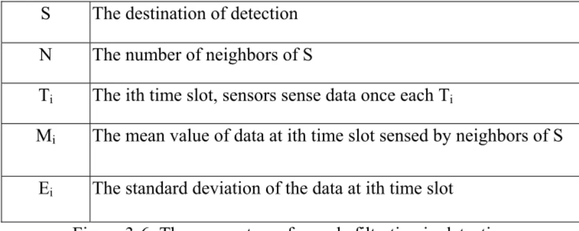
trust them as voters. According to retirement 7, the numbers of compromised neighbors are less than half of a node’s neighbors in WSNs. Figure 3-6 shows the parameters used by following steps.
1. After receiving the data from non-cluster-heads, cluster-heads compute the Mi at each time slot Ti. (the number of time slots is the same as that
in the look-up table of each sensors)
2. Find the half of data set at Ti that most close to the Mi. According to
requirements, the neighbors who transmit these data are the trust voters. 3. In order to judge the remainders is worthy to be trusted or not, we use
the standard deviation Ei to identify. If the value of the difference e from
Mi to data (e = Dij - Mi) is less than or equal to Ei (i.e. e <= Ei), we then
consider that node which transmit that data as a legal voter. The reason why choose Ei to identify whether the remainders are trustful or not is
that the standard deviation Ei represents the arrangement of data. If
standard deviation is high, it means the range of data spread loosely and vise verse. Furthermore, all normal density curves satisfy the following property which is often referred to as the Empirical Rule. 68% of the observations fall within 1 standard deviation of the mean, 95% of the observations fall within 2 standard deviations of the mean, 99.7% of the observations fall within 3 standard deviations of the mean. Thus, for a normal distribution, almost all values lie within 3 standard
deviations of the mean.
4. The chosen voters of each Ti may be different. We chose the ones who
were chosen most of the time.
5. After processing these three steps, the data of chosen voters would be the trustful samples.
If sensors sense more than one data type, the sensor would mark the data type of event and the detection process would go onto that data type.
Figure 3-6: The parameters of sample filtration in detection
3.2.2 Reasonable Data Range Analysis
When cluster-heads know who the voters of the detection destination are, they can compute the reasonable data range of the destination at each time slot. We use regression analysis technique to make cluster-heads achieve that task.
In order to adjust the data of voters into reasonable range, the regression technique will help that. Figure 3-7 shows the data structure of regression analysis. When cluster-heads get the data (i.e. Dij) of voters at each time slots,
they will compute the mean value Mi of each voter’s data and the mean value
mi of data at each time slot.
The effect of sensors ai and the effect of Tj, bj would be:
a = m – M S The destination of detection N The number of neighbors of S
Ti The ith time slot, sensors sense data once each Ti
Mi The mean value of data at ith time slot sensed by neighbors of S
(j is the number of time slots in look-up table of each sensor) bj = Mj – M (i is the number of voters)
Then we compute the fitted value D’ij of each Dij:
D’ij = M + ai + bj
After compute the fitted value D’ij of each Dij, we would have the identical
form of data at each time slot. But these are not the final result of range. We have to consider the residential differences between Dij and D’ij. The
reasonable data of detection destination should be in the range of the data value provided by voters, so we must add the residential differences to D’ij.
D”ij = D’ij + (D’ij – Dij) = 2D’ij – Dij
Finally, we find the up-bound Uj and low-bound Lj of data D”ij at each
time slot Tj and these would be the reasonable range (from Uj to Lj at Tj).
3.2.3 Judging of Compromised Nodes
When the cluster-heads want to detect the non-cluster-heads by judging whether they transmit spoofed data or not, they can use the data of their neighbors to achieve detection. After processing first and second steps of the scheme, the cluster-heads then get the reasonable range of data value to judge the destination. However, it is not correct that if only one data transmitted by destination was out of reasonable range, the cluster-heads would consider the destination as a compromised one. There should be a trustworthy formula to make the decision.
Let the trustworthy value of sensor Si is Wi. If the data of destination at
time slot Tj is out of reasonable range, then:
Wi = Wi – ρj × e- (i.e. e- is the effect of un-trustful value.)
If ρj < 1
Then ρj = ρj-1 + p (p is pre-defined relation probability).
Else ρj = 1.
If the data of destination at time slot Tj is inside the reasonable range, then:
Wi = Wi + e+ (i.e. e+ is the effect of un-trustful value.)
After detecting j times, we should consider the trustworthy value Wi of sensor
Si. If Wi is less than the standard threshold, Si has been compromised and vise
4. Evaluation
In this section, we first analyze the environment where the
simulations process in. Second, we show the result of our
simulations and discuss several factors that can probably influence
the results. Finally, we give a list of security discussion to our
scheme.
4.1 Environmental Analysis
The environment of our scheme should be based on the architecture of clustered organized wireless sensor networks. Contract to the traditional clustered WSNs, the action of clustering begins after the time that event occurred and locates within the isoclusters. As a consequence, the geographical locations of clusters are just right on the locations of events. So the range of data values is limited into a small scope. And the precision of detection for compromised nodes would be reasonable. But there are still two problems of our dynamic clustering environment.
1. What is the size of clusters are suitable for the scheme?
2. What is the relation between the isoclusters and the number of clusters?
First, we should define our analytical environments:
over an area R = [0,L]2 in the network. In figure 4-1, each distance of the side of grids is d. The hop counts which transmission between adjacent position nodes is one hop away.
Following are the proof and analysis of these two problems.
1. In the HEED protocol, the number of hop counts from non-clustered heads to cluster-heads is 1. The smaller size of cluster, the higher precision of the scheme. But one thing we should know that if the numbers of sensor in one cluster are too small, the performance of clustering would very low. The optimal number of the sensors in the cluster is 9. In depend of the locations that events occurred, the time of clustering would change. Figure 4-2 shows one cluster of the WSNs in our environment.
The size of one-hop cluster in the point of geographical view is: (d + d + d)2 = 9d2.
2. The number of clusters depends on the size of isoclusters. According to previous discussion, the size of one cluster in the point of geographical view is 9d2. Assume that events occurred and expend the range, we use the number of hop counts n (from the middle to the sides of the isocluster) to represent the size of isoclusters. When the range expends to n hops away, it consists of (2n+1)2 nodes. Figure 4-3 show the numbers of sensors in the case of one hop range and two hops range in the point of geographical view.
Then we know the number of clusters in n hops is: (2n + 1)2 / 9
We use the generating function to represent all conditions of the cluster numbers︰
The answer of the statement is:
The maximum of n could be unlimited, so the statement can be represent as︰
The coefficient of Xn is the number of clusters in the n hops range of isocluster. The statement is dispersed. That means the numbers of all cases with n hops range are unlimited.
The statement X2+6X+1 / 9(1-X)3 represents the series of the number of clusters in 1, 2, 3… n ….∞ hops range.
4.2 Simulation Evaluation
The environment of our simulation is randomly spread N sensor nodes in an area R[0,L]2 and the events occurred randomly anywhere inside R. The
size of isoclusters may expend or reduced as time go by. The clusters inside the isoclusters would break up or get new ones as the variation of the range of isocluster. If the events occurred and dismissed quickly, the action of clustering would cause down the performance of the networks. So we define the time threshold T that when events occurred exceed T, the action of clustering begins. The time threshold T in our scheme is the time that the size of isocluster exceeds two hops away in the networks. So the value of T is case by case in the simulation.
We used TDMA with IEEE 802.15.4 ZigBee Mac protocol for our simulation environment. The size of look-up table of sensors in our simulation is 20. In other words, the numbers of samples which process detection once by clustered-heads of each voter are 20. There are 10 rounds of detection, once each time slot. So there are 200 data must be transmitted from non-clustered-heads to clustered-heads each case.
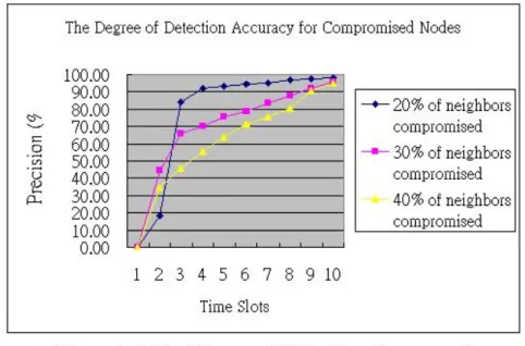
There are three cases of our simulation. Each of which were process over 200 times. We let the nodes compromised 20%, 30%, 40% of neighbors of each node. So there are N/5, 3N/10, 2N/5 compromised nodes between N nodes spread in the network. The best case in our simulation is about 98.10% detection rates in 20% compromised case. According to that graph, we can see the higher precision the later time slot. Because the numbers of compromised nodes inside the network are much less than other case, the relation of geographically locations between compromised nodes does not apparently influence the result. So the better precision occurred at the less numbers of compromised nodes in the networks. There is another one factor that could also influence the result. That is the behavior of compromised nodes. The ones who were compromised might not transmit fabricated contents of message all the time. They can sometime fabricate data and sometime tell the truth. When the value of trustworthy is almost below the threshold, they can tell the truth until the value of trustworthy recovering. That is why some compromised nodes can not be detected. On the other side, the actions which caused down the performance of the network done by compromised nodes would be limited. That’s the goodness of our scheme. The scheme not only detects the compromised nodes inside the range of clusters but also limited the damages caused by compromised ones into 1-hop cluster.
One thing should be noticed in the figure 4-4 is that the detection precisions of 20% case before time slot 3 is less than others. One of the reasons is probably the number of compromised nodes. The probabilities of compromised nodes that fabricate the message most of the time and make the values of trustworthy decreased rapidly below the threshold in higher percent of compromised cases are relatively higher than less ones. The other reasons are the size of isocluster and the relative geographical locations between compromised nodes…etc.
Figure 4-5 represent the detection rate of compromised nodes independently in each slot. By observing that, we can know the highest precision of detection rate is at time slot 3 of figure 4-5 and the largest
variation of detection rate in figure 4-4 is also from time slot 2 to time slot 3.
The time slot 2~3 is the threshold that the stupid (fabricate messages without considering the factor of trustworthy value) compromised nodes were be detected. The scenario does not mean these stupid compromised nodes were always detected from time slot 2 to time slot 3. It means that the stupid compromised nodes were usually detected earlier than smart ones (the ones who do not transmit fake message all the time and consider the effect of trustworthy values).
The ratio of detection on each case from time slot 2 to time slot 3 is: 84% for 20% compromised neighbors, 65.7% for 30% compromised neighbors and 46% for 40% compromised neighbors. At time slot 4, the ratio of detection for 40% compromised of neighbors is 55.5% (see figure 4-4). This represents that most of compromised nodes can be detected in early time slots and the range of detection variation will not vary so much. After that time slot, the remainder compromised nodes would consider the factor of trustworthy values as an important detected element. These conditions were more apparently in more compromised nodes’ cases of the network.
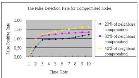
Figure 4-6 shows the false detection rate for compromised nodes. We can see the worse case in the scheme is 1.21%. That means that there are 1.21 normal nodes of the detected compromised nodes.
The better results occurred at fewer compromised nodes cases of the simulation. This is reasonable, because the numbers of compromised nodes in higher precision case are relatively less. The influence of geographically locations between compromised nodes for the result is not so much than more compromised nodes’ case. We can say that the false detection rate of compromised nodes is relative direct proportion to the number of compromised nodes.
Figure 4-7 show the false detection rate independent of each time slot.
intrusion detection system in wireless sensor network [22]. Figure 4-8 shows the effectiveness of data alteration detection compared with the decentralize IDS. We can see that the detection effectiveness of decentralized IDS decrease when increasing the buffer size. The voting based detection would not cause down rapidly as the change of buffer size.
We also evaluate the effect of traffic between clustered WSNs and un-clustered WSNs. There are ten time slots in the evaluation. We use the HEED protocol to clustering, and gather statistics with the number of the packets. The packet sums of each time slot is representing that the number of transmissions which each node transmits one packet. This condition is not usually occurred in the network. Because the sensors do not sense data in each time slot, they sleep ordinary. When it needs to be sensed, the sensors wake up and work. Figure 4-9 shows the simulation result.
5. Security Analysis
We provide a statistical voting scheme for detecting compromised nodes to protect inside attacker from modifying or fabricating data. Before analyze the security prosperities of our scheme, we should define the variables and functions of the environment first.
The scheme is implemented under the clustered WSNs. We define that there are n nodes in a 1-hop cluster with range r. Each cluster has a designated cluster head, with loss of generality, defined as V1. Other nodes
are defined as Vi, where i = 2, …, n. The trustworthy value of Vi is defined as
Wi and S is the threshold used to determine whether a node is compromised
or not. When V1 detect that Vi transmitted a fake message, V1 decreased the
value of Wi. We define the action of decreasing as d(Wi). C is represented as
the set of all compromised nodes in WSNs. The action of detection from V1
to Vi is defined as the function f(Vi) and the reasonable data range of Vi is Ri.
If f(Vi) = 1 then Vi is detected as a compromised one and vice verse. The
range of damages caused by compromised node Vi is Di. Vi ÆfV1 means the
message M transmitted by Vi was fabricated and vice verse Vi ÆtV1.
Following descriptions are the secure properties of our scheme. First, we discuss the influence of probable behaviors of compromised nodes to our scheme. Theorem 1 states that for all cluster members, there exists a reasonable data range which cluster-head can use it to execute detection. If compromised ones transmit fabricated message, cluster-head can discovered that and trustworthy values of them would be decreased. Till the values of trustworthy were less than the threshold, the source would be considered as a compromised node. Theorem 1. ∀Vi, ∃Ri Æ f(Vi), (Vi ∈ C) ∧ (Vi Æf V1) Æ f(Vi) = 1. Proof: ∵ (Vi ∈ C) ∧ (Vi Æf V1) Æ M ∉ Ri Æ (M ∉ V1) ∧ d(Wi) Æ (Di ⊆ r) ∧ (Wi < S)
Æ f(Vi) = 1
However, the compromised ones may not always report fake messages without noticing the trustworthy value. As describe in theorem 2, for all cluster members, there exists a reasonable data range which cluster-head can use it to execute detection. If compromised ones transmit fabricated message, cluster-head can discovered that and trustworthy values of them would be decreased. If the values of Wi almost approach to S, nodes would tell the truth
again. They will not be considered as compromised ones. But the fake messages were still dropped and the damages caused by compromised ones were still limited within 1-hop clusters.
Theorem 2. ∀Vi, ∃Ri Æ f(Vi), (Vi ∈ C) ∧ (If Wi S, then Vi ÆtV1,
else Vi Æf V1) Æ (Di ⊆ r) ∧ (f(Vi) = 0).
Proof:
∵(Vi ∈ C) ∧ (If Wi S, then Vi ÆtV1, else Vi Æf V1)
Æ (Wi > S) ∧ If((Vi Æf V1) Æ (M ∉ Ri))
Æ (Wi > S) ∧ If((Vi Æf V1) Æ (M ∉ V1))
Æ (Di ⊆ r) ∧ (f(Vi) = 0)
Because the sensed data are originally transmitted to cluster-heads and the detection is proceed by cluster-heads, the process of our scheme does not cause additional packet transmission. In theorem 3 we define TD as the extra
packet transmission caused by statistical voting scheme. The action that cluster-head computes Ri is defined as hvi(). The statements of theorem 3 are
that for all cluster members, there exists a reasonable data range which cluster-head can use it to execute detection. The messages from cluster members are originally transmitted to cluster-head. Cluster–head then uses them to compute Ri, so there is no need for extra packet transmission.
Theorem 3. ∀Vi, ∃f(Vi) Æ !∃TD.
Proof: ∵f(Vi)
∵ (Vi ÆfV1)∨ (Vi ÆtV1) ∉ TD
Æ !∃TD
The scheme is executed within 1-hop cluster. If the compromised node transmit the fake messages, that will be detected by cluster-heads. So the damages caused by compromised ones will not spread between clusters. In theorem 4, We define rj as the range of different clusters where j =1,2,3…..
Theorem 4. ∀rj, ∃DiÆ (Vi ∈ rj) ∧ (rj∩ rk = φ), Where i ≠j Æ (Dj ∈ rj) ∩ (Dj ∈ rk) = φ. Proof: ∵(Vi ∈ rj) Æ∃f(Vi) Æ(Dj ∈ rj)
Accord to Theorem 1 and Theorem 2 Æ Dj ∉ rk contradict the claim
Æ Dj =φ
As the proof of these theorems, we demonstrate that the statistical voting scheme can provide strong protection against compromised nodes..
6. Conclusion
In this paper we present a statistical voting scheme for detecting
compromised nodes. By means of statistical analysis, we compute the reasonable range of data to find the inside attackers. Most conventional methods address these problems at a location several hops away from the attacker, which results in high resource consumption and the spread of damage across the network. Under the framework of clustered wireless sensor networks, the statistical voting scheme can not only detect the compromised nodes but also limit the damages within a 1-hop cluster. Because the scheme is proceed by clustered-heads, it would not waste extra transmission effort in the network. Through the evaluation and security analysis, it is proved that our works provide strong protection against compromised nodes.
By stating a critical problem of our scheme, we also consider the following extension as possible future works. If the cluster-heads were compromised, the opposite clusters are not able to detect the compromised nodes. In order to solve that problem, we can apply the statistical voting scheme to the inter-clustering. Cluster-heads can detect compromised ones with each other. We will further improve the scheme, by designing and choosing the best methods in these aspects, make it more resilient and efficient.
7. Reference
[1] N. Vlajic and D. Xia, “Wireless Sensor Networks: To Cluster or Not To Cluster?,” in Proceedings of the 2006 International Symposium on a World of Wireless, Mobile and Multimedia Networks, pp. 258-268, Jane 2006.
[2] J. Y. Cheng, S. J. Ruan, R. G. Cheng, and T. T. Hsu, “PADCP: Power-Aware Dynamic Clustering Protocol for Wireless Sensor Network,” Wireless and Optical Communications Networks, 2006 IFIP International Conference on, pp. 6-, April 2006.
[3] M. Yu, A. Malvankar, and L. Yan, “A New Adaptive Clustering Technique for Large-Scale Sensor Networks,” Networks, 2005. Jointly held with the 2005 IEEE 7th Malaysia International Conference on Communication, 2005 13th IEEE International Conference on, Vol. 2, pp. 6-, Nov 2005.
[4] C. Y. Wen and W. A. Sethares, “Automatic Decentralized Clustering for Wireless Sensor Networks,” EURASIP Journal on Wireless Communications and Networking, 2005.
[5] H. Su and X. Zhang, “Optimal Transmission Range for Cluster-Based Wireless Sensor Networks With Mixed Communication Modes” in Proceedings of the 2006 International Symposium on a World of Wireless, Mobile and Multimedia Networks, pp. 244-250, Jane 2006. [6] S. Bandyopadhyay and E. J. Coyle, “An Energy Efficient Hierarchical
Clustering Algorithm for Wireless Sensor Networks”, INFOCOM 2003. Twenty-Second Annual Joint Conference of the IEEE Computer and Communications Societies. IEEE, Vol 3, pp. 1713-1723, April 2003. [7] O. Younis and S. Fahmy, “HEED: A Hybrid, Energy-Efficient,
Distributed Clustering Approach for Ad-hoc Sensor Networks,” IEEE Transaction on Mobile Computing, Vol. 4, Issue 4, Oct-Dec 2004.
[8] M. J. Handy, M. Haase, and D. Timmermann, “Low Energy Adaptive Clustering Hierarchy with Deterministic Cluster-Head Selection,” Fourth IEEE Conference on Mobile and Wireless Communications Networks, Sep 2002.
[9] K. Sun, P. Peng, and P. Ning, “Secure Distrubuted Cluster Formation in Wireless Sensor Networks,” in Proceedings of the 22nd Annual Computer Security Applications Conference (ACSAC’06), pp. 131-140, Dec 2006.
[10] K. W. Jang, S. H. Lee and, M. S. Jun, “Design of Secure Dynamic Clustering Algorithm using SNEP and µTESLA in Sensor Network,” Proceedings of the 2006 International Conference on Hybrid Information Technology, Vol 2, pp. 97-102, Nov 2006.
[11] A. Perrig, R. Szewczyk, J. D. Tygar, V. Wen, and D. E. Culler, “SPINS: Security Protocols for Sensor Networks,” Wireless Networks, Vol 8, Issue 5, pp. 521-534, Sep 2002
[12] G. Dini and I. M. Savino, “Scalable and Secure Group Rekeying in Wireless Sensor Networks,” in Proceedings of the 24th IASTED international conference on Parallel and distributed computing and networks, pp. 84-88, Feb 2006.
[13] J. H. Li, R. Levy, M. Yu and B. Bhattacharjee, “A Scalable Key Management and Clustering Scheme for Ad Hoc Networks,” Proceedings of the 1st international conference on Scalable information systems, May 2006.
[14] G. Dini and I. M. Savino, “Scalable and Secure Group Rekeying in Wireless Sensor Networks,” in Proceedings of the 24th IASTED international conference on Parallel and distributed computing and networks, pp. 84-88, Feb 2006.
[15] M. Ma and H. M. Keng, “Resilience of Sink Filtering Scheme in Wireless Sensor Networks,” Source Computer Communications, Vol 30, Issue 1, pp. 55-65, 2006.
[16] H. Yang, F. Ye, Y. Yuan, S. Lu and W. Arbaugh, “Toward Resilient Security in Wireless Sensor Networks,” in Proceedings of the 6th ACM international symposium on Mobile ad hoc networking and computing, pp. 35-45, May 2005.
[17] P. De, Y. Liu and S. K. Das, “Modeling Node Compromise Spread in Wireless Sensor Networks Using Epidemic Theory,” in Proceedings of the 2006 International Symposium on a World of Wireless, Mobile and
Multimedia Networks, pp. 237-243, Jane 2006.
[18] F. Li and J. Wu, “A Probabilistic Voting-based Filtering Scheme in Wireless Sensor Networks,” Proceeding of the 2006 international conference on Communications and mobile computing, pp. 27-32, July 2006.
[19] F. Ye, H. Luo, S. Lu, and L. Zhang, “Statistical En-route Filtering of Injected False Data in Sensor Networks,” IN Selected Areas in Communications, IEEE Journal on, pp. 839-845, Volume 23, Issue 4, April 2005.
[20] S. Zhu, S. Setia, S. Jajodia, and P. Ning, “An Interleaved Hop-by-Hop Authentication Scheme for Filtering False Data in Sensor Networks,” IN IEEE Proceedings of Symposium on Security and Privacy 2004, 2004, pp.259-271.
[21] H. Yang, F. Ye, Y. Yuan, S. Lu, and W. Arbaugh, “Toward Resilient Security in Wireless Sensor Networks,” In ACM Proceedings of MobiHoc 2005, pp.34-45, 2005.
[22] A. P. R. da Silva, M. H. T. Martins, B. P. S. Rocha, A. A. F. Loureiro, L. B. Ruiz, and H. C. Wong, “Decentralized Intrusion Detection in Wireless Sensor Networks” Proceedings of the 1st ACM international workshop on Quality of service & security in wireless and mobile networks, pp. 16-23, Oct 2005.
[23] O Dousse, C. Tavoularis and P. Thiran, “Delay of Intrusion Detection in Wireless Sensor Networks,” in Proceedings of the seventh ACM international symposium on Mobile ad hoc networking and computing, pp. 155-165, May 2006.
[24] I. F. Akyldiz, W. Su, Y. Sankarasubramanian and E. Cayirci, "A survey of sensor networks," IEEE Communications Magazine, pp. 102-114, August 2002.
[25] T. Roosta, S. Shieh and S. Sastry, “Taxonomy of Security Attacks in Sensor Networks and Countermeasures,” IEEE International Conference on System Integration and Reliability Improvements, Hanoi, Vietnam, pp. 13-15 Dec 2006.
Attack and Countermeasures” in Proceedings of the First IEEE. 2003 IEEE International Workshop on, pp. 113-127, May 2003.