建構互動式腦神經網路資料庫之神經基因表現圖譜及其三維影像處理系統---細緻結構之萃取與分析(子計畫三)(III)

(1)

行政院國家科學委員會專題研究計畫成果報告

建構互動式腦神經網路資料庫之神經基因表現圖譜及其三

維影像處理系統--細緻結構之萃取與分析(子計畫三)(3/3)

研究成果報告(完整版)

計畫類別：整合型計畫編號： NSC 97-2627-B-009-001- 執行期間： 97 年 08 月 01 日至 98 年 07 月 31 日執行單位：國立交通大學資訊工程學系（所）計畫主持人：荊宇泰共同主持人：林志陽計畫參與人員：此計畫無其他參與人員處理方式：本計畫可公開查詢

中華民國 99 年 01 月 05 日

(2)

0

行政院國家科學委員會補助專題研究計畫成果報告

建構互動式腦神經網路資料庫之神經基因表現圖譜及其三維

影像處理系統--細緻結構之萃取與分析(子計畫三)

計畫類別：□ 個別型計畫■ 整合型計畫

計畫編號：NSC 97-2627-B-009-001－

執行期間： 97 年8 月1 日至98 年7 月31 日

計畫主持人：荊宇泰

共同主持人：林志陽

計畫參與人員：

成果報告類型(依經費核定清單規定繳交)：□精簡報告■完整報告

本成果報告包括以下應繳交之附件：

□赴國外出差或研習心得報告一份

□赴大陸地區出差或研習心得報告一份

□出席國際學術會議心得報告及發表之論文各一份

□國際合作研究計畫國外研究報告書一份

處理方式：除產學合作研究計畫、提升產業技術及人才培育研究計畫、列

管計畫及下列情形者外，得立即公開查詢

□涉及專利或其他智慧財產權，□一年■二年後可公開查詢

執行單位：國立交通大學

中華民國98 年7 月31 日

附件一

建構互動式腦神經網路資料庫之神經基因表現圖譜及其三維影像處

理系統--細緻結構之萃取與分析(子計畫三)

Yu-Tai Ching Chih-Yang Lin

(3)

I 摘要本計畫應用影像處理技術，擷取果蠅腦共軛焦顯微鏡影像中的三維細微結構，例如神經結構以及橢圓體(ellipsoid body)。我們也定義了一個果蠅腦橢圓體中心為心的坐標系統。並將這些技術產生的結果用於建構世界第一個果蠅腦資料庫。為了發展下一個果蠅腦資料庫，我們也發展了一個新的果蠅腦warping技術。該技術可以精確的將Ａ果蠅腦warp進另一個Ｂ果蠅腦，並將Ａ果蠅腦中的神經帶入B果蠅腦中。同樣技術也用於antenna lob中local neuron的warping及分析。執行本計畫，我們已經為將來的果蠅研究工作奠定基礎。另外在神經萃取的工作之後，我們已經發展出比較神經的方法，該方法對研究神經發育將有重要幫助。關鍵詞：果蠅腦、共軛焦顯微鏡、神經比對

ABSTRACT

We apply computer techniques to extract fine structures, such as neuron and ellipsoid body, from the fly brain confoal microscopic images. We have defined a coordinate system for the fly brain that the coordinate system is centered at the center of the ellipsoid body. These result has been used in building the first fly brain database in the world. In order to develop the next version of the fly brain database, we also developed a warping algorithm that warps one brain to the other accurately. In the mean time, we can warp the second channel neuron in the source fly brain to the target fly brain. These works have established important foundation for the researches of the fly brain. The warping algorithm was also applied to analyze the connectivity of local neuron in antenna lobe. Following the neuron tracing algorithm, we developed a neuron comparison algorithm that can be applied to study the development of neuron.

Keywords: Drosophila, neuron tracing, brain warping, confocal microscope, fly database, neuron comparison

(4)

II

2.4.1

List of Figures

Fig. 1. The projection neuron in Drosophila’s calyx ... 3

Fig. 2. This figure shows the Drosophila’s projection neuron in the lateral horn . 3 Fig. 3. A neuron around the ellipsoid body ... 4

Fig. 4. The Ellipsoid body... 5

Fig. 5. Two fly brains are warped into target fly brain ... 6

Fig. 6. Two optic nerves of albino tadpole ... 8

Fig. 7. Six local neurons are warped into a target antenna lobe ... 9

(6)

- 1 -

1. Introduction

This project is a subproject of Professor Chiang’s fly group that studies the brain of

Drosophila. In this subproject, we developed methods and systems that help to build a

fly brain database in the past three years.

The images studied were acquired from confocal microscopy. Since this kind of images only serves to a small research community, there were not many similar previous works. Most of the groups worked on medical images such as CT or MR. Our contributions may not be judged from engineering point of view. But we are confident that we have made contribution to the research work of neural science.

The algorithms and software system we have developed in this project are listed in the following.

1. A neuron tracing algorithm: We have worked on neuron tracing algorithm for a long time. We started with vessel tracing algorithm. Since the neurons presented in image is very different from the vessel. The vessel tracing algorithm did not work. We then developed a tracing algorithm based on the gradient vector flow snake. This algorithm worked but need user interface. The algorithm developed in this project was based on the graph algorithm. We find the shortest path to establish the branches and to construct the neuronal tree. The algorithm has been applied to trace more than 5,000 neurons and has shown the robustness of the algorithm.

2. Define a coordinate system for the fly brain: We defined a coordinate system for the fly brain. The coordinate system is centered at the center of the ellipsoid body. This coordinate system allows us to align and to normalize the size of fly brain. This coordinate system also serves as a basis for our newly developed fly brain warping algorithm.

3. Developed a new warping algorithm: Professor Chen, Yun-Shen and we developed a new warping algorithm and applied the algorithm to fly brain work. This algorithm is developed based on the affine transformation and Radial Basis Function (RBF) deformation, to the fly brain research. This warping algorithm can warp fly brain from one to the other accurately. Since

the way of warping is recorded, we can warp the 2nd channel neuron to the

target brain. That means we can deposit many neurons acquired from different flies to a template. Thus we have chance to study the connectivity between neurons. This method will serve as the key operation in the next version fly brain database.

(7)

- 2 -

neuron is important. For example, a fly after training could change the morphology of a specific neuron. Another important research area is to study the plasticity of a neuron. For example, scientists are interested in the changes of a neuron as an animal grows up. We can trace the neuron and present the neuron as a tree structure rooted at soma. To compute the differences between a pair of trees can be done by solving the tree isomorphism problem. Unfortunately, computing tree isomorphism is intractable. In this project, we take advantage of the geometry information and developed a neuronal tree comparison algorithm using the greedy approach.

5. Try to establish the connectivity of local neuron in antenna lobe: There are around 50 glomerulii in the antenna lobe in the fly brain. There are local neurons that each of those has branches in some of the glomerulii. Different neuron with branches in the same glomerulus can be considered they are connected. Compute the neural network can help us understand how the neurons in antenna lobe “compute”. We have partial result that warp from one antenna lobe to another could lead us to the result that constructs the neural network.

In the following section, we present our results obtained in this project.

2. Results

2.1. A Neuron Tracing Algorithm.

The proposed method is designed based on an optimization technique in graph algorithms. The accumulated experiences from our previous work, we found it is difficult to trace neurons in 3D volume. It is also difficult to design a thinning algorithm in 3D space. But there are effective thinning algorithms in 2D space. From these observations, we developed a method that calculates the 2D skeleton of neuron in 2D space first. The true 3D skeleton of neuron is then computed from the set of 2D skeletons.

We describe the algorithm in the following.

1. We compute the skeleton of neuron in each slice. Note that although the neuron is a connected component in the volume data, there could be more than one connected component in a slice.

2. For the skeleton in each slice, we determine the set of end points in the skeleton. Note that, an end point may or may not be a true end point of the neuron fibers in 3D space. If a 2D end point is not a 3D end point, this point is generally close to the neuron fiber that moves from one slice to the other. We set a deviation that can eliminate such kind of points.

(8)

3. The third step is to compute the neuronal structure from the set of 2D skeleton. We assume that the center point, p, of the soma is available. Suppose that we have the shortest path from between all of the points to p. The farthest 2D end point, q, from p should be the true 3D end point. We compute the path from p to q and trim the 2D end points that are close to the path from p to q (since there are likely not to be the true 3D end points). This process is carried out iteratively. In each iteration, we compute the longest path from p to a 2D end point. We then trim out those 2D end points close to the path. This process iterates until the set of 2D points is empty.

This method has been applied to more than 5000 sets of data. In almost all of the cases, we could achieve very good result. Only a small portion of the data sets could not be done successfully. We believe those data sets were acquired by an individual and the quality of that images are much worse than the others. The figure 1, 2 and 3 show the tracing results.

Figure. 1. The projection neuron in Drosophila’s calyx.

Figure. 2. This figure shows the Drosophila’s projection neuron in the lateral horn.

(9)

Figure 3. A neuron around the ellipsoid body.

2.2 Define a Coordinate System for the Fly Brain.

We defined a coordinate system for the fly brain. The coordinate system is a orthogonal coordinate system that centered at the center of the ellipsoid body. To segment the ellipsoid body, the user has to provide a bounding box that encloses the region of interest. The segmentation algorithm is developed based on the intensity difference between the region of interest and the background. We then use the property that the shape of this neuropil is a donut shaped object. Once the voxels in the ellipsoid body is determined, since it is donut-shaped, we can compute a point which is the best approximation of the center of the ellipsoid body. The center of the ellipsoid body is defined to be the center of two co-centric circles, C1 and C2. Both of C1 and C2 are cantered at the center of the ellipsoid body and C2 enclose C1. C1 is the largest empty sphere and C2 is the largest enclose sphere of the ellipsoid body. Two segmentation results are presented below.

(10)

Figure 4 The Ellipsoid body is shown in yellow color.

As mentioned previously, the center of the coordinate is defined to be the center of co-centric center. The three axes are obtained the principal component analysis of the gray scale volume data.

2.3 Brain Warping

Given two fly brains, we compute the center and the axes for each brain. The preliminary alignment of two brains are aligned so that

1. Their centers are coincide and 2. Three axes are aligned.

Since axes and center are defined, a bounding box enclosing the brain can be defined. The bounding box serves as a scaling parameter to scale up or down of the brain. This alignment process serves as a preliminary alignment.

A more accurate alignment/warping can be achieved by a method developed by Professor Chen’s ( 陳永昇教授 ) lab. The alignment starts with two affined transformations, the first is a 7-degree of freedom affine transformation and the second is a 12-degree of freedom transformation. The matrices define the two affine transformation is obtained by an optimization process to compute the entries in the matrix.

Following the affine transformation, a non-rigid transformation based on Radial Basis Function is applied. It matches two volumes voxel-wise to achieve the warping process. The non-rigid transformation produces three matrices. Each of those describes one of the x, y, and z components that a voxel deforms. By using the three matrices, we are able to bring the second channel neuron into another brain.

(11)

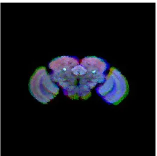
Figure 5 Two fly brains are warped into target fly brain (three fly brain ware warped together). This result show that the warping algorithm us accurate.

2.4 Neuron Comparison 2.4.1 Rigid body Registration

There have been many registration methods reported and applied to the biomedical images. Roughly they can be divided into two classes, rigid body registration and nonrigid registration. Since our task is to observe the growing process, the rigid body registration is a naturally choice. We adopt the classic Iterative Closest Points (ICP) method to register the inputs. When a pair of neuron images, the source neuron image and the target neuron image, are given, we firstly sample only 25% points from the boundary surface of the neuron randomly to form the point cloud representation of the neuron.

2.4.2 Two-level Matching

After the centerline is traced out, both the branches of the source neuron, NeuronS and the branches of the target neuron, NeuronT are reconstructed. The neuron branch is defined as the origin dendritic root, soma to the free tip of a dendritic terminal and the length of the branch is de_ned as the same as the "path length" defined by Van der Loos. By the descending order of the neuron length, we make the longer-length prefered clusters. Iteratively the longest unclustered branch is picked as the center trajectory and an extend radius is set then this forms a tube. And every unclustered branch which is covered more than 80% by the tube is collected into the same cluster,

Gi

For convenience, hereafter the variable with subscript S indicate that it is used to

describe the NeuronS and the variable with subscript T is used to describe the NeuronT

(12)

respectively. Along each branch curve, C, from the soma to tip, we sample the points,

Pi every unit-length. Then complete bipartite graph, KM,N is constructed with the

weighting function defined as below:

- 7 -

⎤

⎡

(1) where (2) and (3)

In Eq. (1), the ||C|| means the arc length of the branch curve and the in Eq. (3) means the regular Euclidean distance between two points. Denote the set of

branches of a neuron as B. W.L.O.G. assume . Let f : BSÆBT be a injective

function and f is the best assignment if

(4)

In the coarse-level matching stage, only the longest branch, Liof Giis considered.

Assume that GpS matches GqT then in the next fine-level matching we look for another

assignment again w.l.o.g. assume , to minimize

(5)

Both f and g can be found in polynomial time when the Hungarian algorithm is applied.

2.4.3 Matching Result

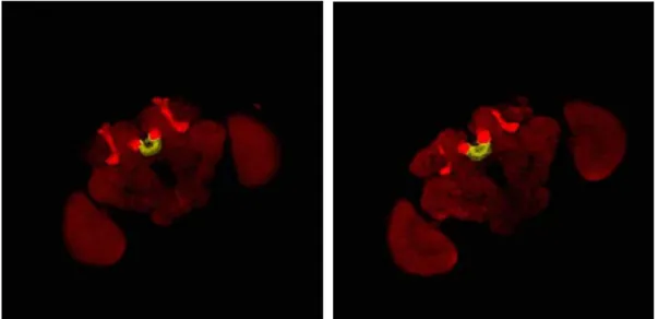
Figure shows the optical nerves of the albino tadpole. The images were taken at two

consecutive time points. The left one was taken at Ti and the right one was taken at

Ti+1. The red filaments shown in both left-hand and right- hand side represent the

alternations.

⎡

|| ||

⎤

) , ( ) T S T T C C C Dis + ) , ( ) , (C_S C_T Dis Pi C Dis =∑ || || , ( ) , ( S S T S C C C Dis C C Weight = T S i ||} , {|| min ) , ( _Si _Tj C P T i S C P P P Dis T j T∈ = || , || i _Tj | | _T S S P P | |B ≤ B

∑

∈ ∈ < ∃ S c B T S c f c fˆ: → ⇒ ( , ˆ( )) S c c weight B B , )) ) (~ B c f weight( ( q T p S | T | p S | | q G G ≤ G G g: →

∑

∈ b weight p S G b g b, ( )) (

(13)

Figure 6. Two optic nerves of albino tadpole. All the neuron centerlines were traced by the algorithm proposed last year

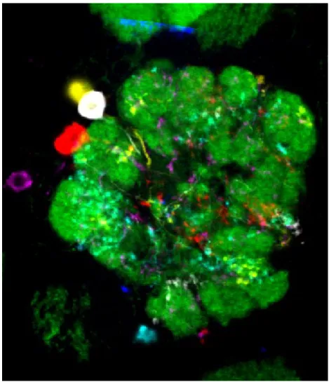
2.5 Connectivity of Local Neurons in Antenna Lobe

The topic is an extension of the warping algorithm but shows a very important research topic. There are local neurons around the antenna lobe. Each neuron has branches to several glomerulii. Scientists believe local neurons conduct computation. To understand how they compute, we must construct the neural network of local neuron.

At the present time, image of only one local neuron can be acquired. Thus, in order to study the connectivity, the only way to establish the neural network is to warp local neurons to a target one.

Warping from one antenna lobe to another is not that easy as to warp a fly brain due to the very vague boundary between glomeruli. To solve this problem, we have design a method that we define a mask for the target antenna lobe. A preliminary result shows that we have good chance to warp all of the local neurons into a target antenna lobe.

(14)

Figure 7. Six local neurons are warped into a target antenna lobe.

3. Conclusion and Discussion

In this project, we developed algorithms to trace neurons, to compare neuron, to warp brain from one to the other. These works established foundation for our future work. The future work will be much more biology oriented, i.e., we shall try to solve biology problem based on the computer techniques developed. We are confident that we (fly research groups and our group) have chance to work on unique work in the world.

Papers published or submitted

1. Ping-Chang Lee, Yu-Tai Ching, H.M. Chang, Ann-Shyn Chiang, “ A Semi-automatic Method for Neuron Centerline Extraction in Confocal Microscopic

Image Stack”, IEEE International Symposium on Biomedical Imaging, 2008