國
立
交
通
大
學
企業管理碩士學程
碩
士
論
文
台灣股市與美國那斯達克的動態相關性分析
Dynamic Conditional Correlation Analysis of
NASDAQ and Taiwan Stock Market
研 究 生:楊士漢
指導教授:周雨田 教授
台灣股市與美國那斯達克的動態相關性分析
研究生:楊士漢 指導教授:周雨田 博士
國立交通大學企業管理碩士學程
中 文 摘 要
世界是平的!全球的經濟脈動,牽一髮而動全身。對台灣股市而言,與美國市 場的相關性最為明顯。在本研究論文中,將針對美國科技類股具代表性的那斯達 克(NASDAQ)綜合指數、台灣大盤指數(TAIEX)以及台灣電子期貨指數(EXF)進行相關 性的研究。本文將運用 Robert Engle 教授所提出著名的動態條件相關性模型 (DCC, Dynamic Conditional Correlation)來針對台灣與美國指數間連動性做深入的探討。 本文內容將針對美國 NASDAQ 綜合指數的隔日報酬(daily close‐to‐close rate of return)是否對於台灣市場具有報酬和波動性的外溢效果(spillover effect)做實證研 究。根據實證結果顯示,不管對於 TAIEX 或是 EXF,NASDAQ 均具有統計的顯著 報酬外溢效果,其中對於台灣市場的隔日報酬影響最為顯著。此外,台灣市場的 隔夜報酬(close‐to‐open rate of return)具有過度反應的現象(overreaction),因為台 灣和美國時差的關係,美國開盤和收盤時台灣並沒有交易,因此,開盤時會受到 美國收盤的狀況產生過夜的漲跌反應,但隨著開盤後,國內資訊的影響性凌駕了 國外資訊,在交易時間中,會回歸到市場應有的價值水準。本研究將將針對台灣 市場的三種報酬率(隔日、隔夜、當日報酬)與美國 NASDAQ 的隔日報酬做相關性 實證。 Keywords: 動態條件相關性, 相關性, 股票市場, 那斯達克, 時間序列Dynamic Condition Correlation Analysis of NASDAQ and Taiwan
Stock Market
Student: Shih-Han Yang Advisor: Dr. Ray Yeutien Chou
Master of Business Administration
National Chiao Tung University
Abstract
The world is flat. The world economies link more and more closely recently. For Taiwan stock market, the most influential markets come from the United States. In this research article, NASDAQ, TAIEX (Taiwan Stock Exchange Index) and EXF (Taiwan Electronic Sector Index Futures) are chosen to estimate the correlations. Professor Robert Engle’s DCC (Dynamic Conditional Correlation) model is employed to model the correlations between each two time series.
The price changes and volatility spillover effects will also be estimated in this article. By the results, the price changes spillover effects from NASDAQ are all significant to both TAIEX and EXF, and the most significant one is the C2C (close-to-close) return. There might be an overreaction on the open price of Taiwan market to the return of NASDAQ. After the overreaction of open price, the market index was adjusted to the proper price within the trading hours. Finally, a trading strategy is proposed here to put theory into practice. We could possibly trade to gain some profit by the correlation between Taiwan and the United States.
Acknowledgements
Within the wonderful two years I spent in National Chiao Tung University, I’ve gotten much help from professors, classmates and friends. I couldn’t finish my duties without the warm hands definitely, including this thesis. First of all, thank Dr. Ray Yeu-Tien Chou very much; Professor Chou gave me so many advices that I could finish the thesis in time. I thank Professor Edwin Tang; he is always enthusiastic, and he is our CHIEF of MBA program. I love all my classmates of NCTU MBA. Hey guys, you are the best. I can’t forget anything I experienced with you in these two years, especially the funny days in Europe. Wish all the classmates have an excellent future. I thank all my friends for the beers, jokes and comfort.
Surely, I should thank all my families for their support, my father told me to seek my own dreams without any fears. More challenges, more efforts should I make. I will always keep the concept in my mind, no matter in school or in my career life. I don’t know how to express my appreciation for you, and I will do my best to do all what I need to do. Thank you very much.
Table of Contents
中 文 摘 要 ... I
ABSTRACT ... II
ACKNOWLEDGEMENTS ... III
1. INTRODUCTION ... 1
1.1
B
ACKGROUND ANDM
OTIVATION OFT
HISR
ESEARCH... 1
1.2
R
ESEARCHO
BJECTIVE... 3
1.3
L
IMITATION OF THER
ESEARCH... 5
1.4
F
RAMEWORK OF THER
ESEARCH... 6
2. LITERATURE REVIEW ... 7
3. METHODOLOGY ... 10
3.1
D
EFINITION OFR
ATE OFR
ETURN... 10
3.2
T
WO‐
STEPE
STIMATIONM
ETHOD... 12
3.3
DCC
M
ODEL... 15
3.4
DCCX
M
ODEL‐
E
XTREMER
ETURNE
FFECT... 19
4.2
S
AMPLES
ELECTION... 21
4.3
D
ESCRIPTIVES
TATISTICS... 22
4.4
R
ESULTS OFT
WO‐
STEPE
STIMATION... 24
4.5
R
ESULTS OFDCC
M
ODELE
STIMATION... 26
4.6
R
ESULTS OFDCCX
‐
E
XTREMER
ETURNE
FFECTS... 29
5. CONCLUSION ... 32
APPENDIX - FIGURES AND TABLES ... 34
F
IGURE1
C
LOSEP
RICE... 34
F
IGURE2
R
ETURNC
HARTS... 35
F
IGURE3
C
ORRELATIONC
HARTS... 39
T
ABLE1
D
ESCRIPTIVES
TATISTICS... 42
T
ABLE2
U
NCONDITIONALC
ORRELATIONM
ATRIX... 43
T
ABLE3
T
WO‐S
TEPE
STIMATION... 43
T
ABLE4
DCC
M
ODELE
STIMATIONR
ESULTS... 47
T
ABLE5
DCCX
M
ODELE
STIMATIONR
ESULTS... 48
1. Introduction
1.1 Background and Motivation of This Research
Investors are looking forward to taking advantage of a price spread between two or more financial markets, such as bonds, stocks, derivatives, commodities and currencies markets. Nowadays, the stock market provides investors an easy-to-liquidate, easy-to-trade market, so investing stocks is one of the most popular investment instruments. Not only the investors, traders but also top tier analysts of investment banking companies are developing many methods to forecast the securities prices, including quantitative and experiential methods. Quantitative methods are based on a mathematical model built to describe the market behaviors. By statistical techniques, a regression curve can be found to fit the historical data with a minimum difference, however, the explanatory power depends upon the adequate selection of independent variables. In statistics, several methods taught us how to select the adequate independent variables, such as forward selection, backward selection, and stepwise selection methods.
Technical analysis of historical data is an example of experiential methods. Ralph Elliot proposed Wave Theory to explain the United States stock markets in 1930s. Elliot
found that the stock prices changed with an observable pattern, and which duplicates in forms of price performance not in price range or time span. No matter which method is employed, the objective is identical, to gain money from the stock markets.
Unfortunately, no one can predict the real price of any stock tomorrow. Because the stock exchange lists the companies owned publicly, the price of the stock is negotiated by the bid and ask price. The bid price stands for the price which buyers are willing to pay, and the ask price is the price at which sellers are willing to sell. The next unpredictable step is called Random Walk in finance. Random walk is a mathematical formalization of a trajectory that consists of taking successive steps in random directions. It implies that the price is like a walking drunkard, the next step depends on the present place he stands in, and we will never know where he will step ahead. The logarithm of stock price follows a continuous random walk, see Lo and MacKinlay (1988). That is to say, it is impossible to forecast the next step of stock price.
Because of the different time zones, there are always stock markets trading all day long around the world. A phenomenon can be observed that the linkages among the stock markets around the world are getting stronger and stronger, especially the dependence upon the stock market indices of the United States of America. Many academic studies show that the spillover effects of return and volatility exist between
the markets, see Darbar and Deb (1997) and Chou, Lin and Wu (1999).
I have cared about the Taiwan stock markets for several years; I could find that the relationship of securities markets between Taiwan and the United States was getting stronger. With the high transparency of international events and trading activities, the events happened in the United States usually could impact the open price of Taiwan stock market. The open price means the first traded price of the trading day. Therefore, I want to study the correlation of the securities markets between Taiwan and the United States and expect to propose a trading strategy based on the correlation.
1.2 Research Objective
Because of the increasing foreign participation in the Taiwan stock market, the linkages between Taiwan stock market and other countries are strengthened, especially the United States stock markets. Spillover effect1 will be studied in this article, including
the price change and volatility spillover effects between Taiwan and the United States markets, and correlation between the two countries’ markets will be modeled as well. The exchange trading indices include several industries, such as manufacturing, information technology, electronics and etc. For example, the United States Dow
Jones index covers 30 listing manufacturing companies, and NASDAQ Composite Index covers over 3600 high-tech companies. Each index stands for its specific industry performance respectively. The chosen industry of this research is the electronic industry. The reason why electronic industry selected is that the electronic industry is a representative one in Taiwan and its traded volume of electronic industry sector is weighted by around 60% of the daily total traded volume of TAIEX. So it is reasonable to choose electronic industry sector on behalf of Taiwan stock market performance. The index chosen is NASDAQ Composite Index (abbreviated as NASDAQ) for the United States stock market and Electronic Sector Index Futures (abbreviated as EXF2) for the Taiwan market. As the name said, the underlying index of
EXF is the Taiwan Stock Exchange Electronic Sector Index. However, the Taiwan Exchange Index (TAIEX) is employed to compare with NASDAQ, too. The research results will show two pair-wise correlations, NASDAQ with EXF and NASDAQ with TAIEX.
The objectives of this research are:
1. The price changes and volatility spillover effect between Taiwan and the United
2 The trading hours of EXF are from 08:45AM to 1:45PM Taiwan time, Monday through Friday of the
regular business days of the Taiwan Stock Exchange. EXF has a daily price limit of +/- 7% of previous day’s close price.
States markets.
2. The correlation of NASDAQ and EXF. 3. The correlation of NASDAQ and TAIEX.
4. Extreme return effects of NASDAQ on EXF and TAIEX.
1.3 Limitation of the Research
The chosen objects, NASDAQ and EXF, are one of the many indices in the United States and Taiwan, respectively. This research provides a method to analyze the correlation between two stock markets, but not a general result for all the markets in the world. Even if for NASDAQ and EXF, the results might be different from the empirical results in this article, because of the time period covered in the sample data. The properties of the data employed in this article will be shown in chapter 4.
1.4 Framework of the Research
The framework of this research article is structured as the flow chart below.
1. Introduction
2. LITERATURE REVIEW
4. Empirical Results 3. Methodology
2. Literature Review
There are many reports or research literatures studying the relationship between two or more time series numbers. Several multivariate GARCH models have been proposed to show the covariance of time series data in the literature, including VECH model, see Bollerslev, Engle and Wooldridge (1995), the diagonal VECH, BEKK model, see Engle and Kroner (1995), and the dynamic conditional correlation (DCC) model, see Engle (2002). The method used in this article is the last one, DCC model.
Grubel (1968) proposed the concept of internationally diversified portfolios. After that, the relationship of assets was taken into account when managing the investment portfolios. In the beginning, the coefficient of correlation of two financial instruments was used to describe their co-movement. A mathematical function is used to describe the relationship between, given one variable, and then the other is determined. It gives a curve that minimizes the overall difference. However, the method is too simplified that many determinant factors are ignored. Then, the concept of time-varying covariance was employed, see Bollerslev, Engle and Wooldridge (1995) for details. Chou, Lin and Wu (1999) employed the multivariate GARCH model to examine the Taiwan stock market price and the volatility linkages with those of the United States.
They found a substantial spillover effect from the United States market to Taiwan market using the Taiwan close-to-open3 returns, because of the incapability of
reflecting the market information into the market price when market is closed. Also, they concluded that the “US induced” volatility amounts to 12 percent to total daily stock volatilities of the Taiwan market.
Darbar and Deb (1997) employed the multivariate GARCH model to examine the linkages among four equity markets – the US market, the UK market, Canada market and the Japanese market. They concluded that the Japanese and U.S. stock markets have significant transitory covariance, but zero permanent covariance. The other pairs of markets examined display significant permanent and transitory covariance. They also concluded that, while conditional correlations between returns are generally small, they change considerably over time, and basing diversification strategies on these conditional correlations is potentially beneficial.
There are also some researches to study the linkage between Taiwan stock market and other counties’. Most of them employed the multivariate GARCH model to analyze the markets. This study differs from them in two respects. First, it uses the dynamic conditional correlation model (DCC model), see Engle (2002), which employs the
3 Close-to-open return means the overnight return, the rate of return of open price and the previous
time-varying dynamic structure into the model, to analyze the markets. It allows the correlation matrix to be time-varying. Second, the scope of this study is specified in two levels, the electronic industry sector index futures and the TAIEX (Taiwan Exchange Stock Index), the correlations between the indices and NASDAQ will be examined respectively. For the empirical results using DCC model, Engle and Sheppard (2001) proposed the theoretical and empirical properties of DCC multivariate GARCH model, however, they took the stock markets within the United States for reference instead of international markets.
3. Methodology
The purpose of this research is to survey the linkage of the stock markets in Taiwan and the United States. First of all, the spillover effects will be estimated. In this article, the two-step estimation method will be employed to model the price changes and volatility spillover effect between the markets. And then DCC model will be used to estimate the correlation. As implied by the name, DCC model is a correlation formula with a dynamic structure, and which takes the time-varying covariance into consideration. The details will be elaborated in the following section.
The analysis software tools used for this article are Microsoft Excel 2007 and Eviews version 5.
3.1 Definition of Rate of Return
The type of rate of return common in use is continuous compounding rate of return, and which is also used in this article. The definition of continuous compounding is shown as the below equation:
ROI ln PP (1) In the equation above, ROI is the return of investment, defined as the natural log of the final price of investment instrument divided by the initial investment value. However,
we multiply the ROI value by 100 times to get the numerical part of the percentage into the following calculation.
In order to count the effect of cut point of stock price in the rate of return, I divided the rate of return into three types, close-to-close (C2C), close-to-open (C2O, overnight return), and open-to-close (O2C, intra-day return) returns, where the C2O return is also called overnight return. The close-to-open means the rate of return of investment is the natural log of the open price of the investment instrument (for example, Wednesday’s open price) divided by the previous trading day’s close price (for example, Tuesday’s close price). By the same token, the elements of the other types of rate of return are shown as the following table respectively.
1. C2C Rate of Return ln P P
′ 100% (2)
2. C2O Rate of Return ln P P
′ 100% (3)
3. O2C Rate of Return ln PP 100% (4) Types of rate of return
close-to-close (C2C) close-to-open (C2O) open-to-close (O2C) Elements
Final Price (Pf) Close price Open price Close price
Initial Price (Pi)
Previous trading day’s close price
Previous trading
It deserves to be mentioned that the rate of return of NASDAQ used in the following methods is the close-to-close one. Because we aim to find out the spillover effect from the United States stock market to Taiwan market, the reference rate of return is fixed, the close-to-close rate of return of NASDAQ. For the comparison object, the various rates of return of Taiwan stock market will be considered in the following analysis respectively.
3.2 Twostep Estimation Method
In order to identify the price changes and volatility spillover effects from the United States market to Taiwan market, I use the two-step estimation method, MA(1)-GARCH(1,1) model, for the two markets, see Chou, Lin and Wu (1999) for details. For the two-step estimation method, we estimate the return and residual first and then estimate the variance. We can estimate the return and residual of the influencing economy (the United States) by uni-variate GARCH model in the first step, and the squared term of resulting residual together with the return are used as the explanatory variables in the mean and conditional variance of the influenced economy (Taiwan) in the second step. The index t is the day time, denoting either the opening or closing time. The WD dummy variable is the weekend effect dummy variable, defined to be 1 as the return covers a weekend (close-to-close and close-to-open return) or a
Monday (open-to-close return) and 0 otherwise. It helps us to identify whether the weekend effect significant or not. Weekend effect4 is a term used to describe the phenomenon in financial markets in which stock returns on Mondays are often significantly lower than those of the immediately preceding Friday. The mathematical formulas of two-step estimation method are shown as below.
R b b WD b e e (5) h E e I a a e a h a WD (6)
The first equation, we call it mean equation, is a MA(1) model. Rit is the market
return for market i at day t, and eit, i=1 and 2, are white noise. The second equation, we
call it variance equation, is a GARCH(1,1) model, eit-12 is the squared term of residual,
and hit-1 is the conditional variance of Rit based on an information set containing all the
price information at day t-1.
4 The weekend effect has been a regular feature of stock trading patterns for many years. A number of
empirical results offer explanations for this market behavior. Some theories suggest that the tendency for companies to release bad news on Friday after the markets close accounts for depressed stock prices on Monday. Others state that the weekend effect might be linked to short selling, which would affect stocks with high short interest positions. Or, the effect could simply be a result of traders' fading optimism
In order to test whether Taiwan market is affected by the United States stock market or not, the most recent United States market return is introduced into the mean equation of Taiwan market return and squared term of the United States market residuals is introduced into the variance equation of Taiwan market return, too. The two markets are indexed by i: 1 for Taiwan market (domestic market), and 2 for the United States market (foreign market), and the model used in this research is defined by following:
R b b WD b e b R e (7) h E e |I a a e a h a WD a e (8)
In the two equations above, the foreign market return and foreign squared term of residual are designed to capture the return spillover and volatility spillover, respectively. If the statistical result of b3 is significant, it implies that a change of price return of the
United States stock market will cause a change of price return of Taiwan market. If the statistical result of a4 is significant, it implies that the volatility spillover effect exists
from the United States market to Taiwan market.
The estimation results will be tested by maximum-likelihood estimation method. Besides the t-statistics for each of the coefficients, the likelihood ratio statistics (LR)
will be computed for joint significance of the coefficients. The Leung-Box Q statistics for the squared normalized residuals will also be computed, denoted as LB-QS. All the estimation results will be arranged in the following chapter.
3.3 DCC Model
Engle (2002) proposed a dynamic structure to analyze the correlation of two time series data, and that is the Dynamic Conditional Correlation (DCC) model, and which is modified from the Constant Conditional Correlation (CCC) model, see Bollerslev (1990), to let the correlation matrix time-varying.. The DCC model was proposed to solve the conditional covariance problems, and that can be simplified estimated by uni-variate GARCH models for each series’ variance process. The DCC model estimates a conditional correlation by employing the transformed standardized residuals from the GARCH estimation step and then estimating the time-varying conditional estimator in the next step. An advantage of DCC model is easy-to-estimate; although it is not linear, it can be estimated simply by two stages based on the maximum likelihood method. This article will show the empirical results of using DCC model to estimate the correlation of NASDAQ and Taiwan market indexes in the chapter 4.
between two series data (r1 and r2 with zero means) traditionally, and those are
defined by:
COV E r ,, r , , (9) ρ , E , , ,
E , E , . (10)
The covariance and correlation are computed by previous data. However, there are two problems, one is too many premature data are used, and the other is that the previous lags assigned equal-weighted will cause the problem of uncoupling correlation estimation.
Here, we consider the DCC model with two assets,
H D R D , where D diag h, , (11)
R diag Q / Qdiag Q / , (12)
Q S ℓℓ′ A B A Z Z′ B Q , (13)
or in a bi-variate model like the empirical case in this article,
q , q , q , q , 1 a b 1 q q 1 a z, z, z , z , z , z , b q , q , q , q , . (14)
In the equations above, Ht is the covariance matrix, Dt is the 2 2 diagonal matrix of
time varying standard deviations from uni-variate MA(1)-GARCH(1,1) models with h on the ith diagonal, and R
t is the time varying correlation matrix. A and B are
represents the unconditional covariance of standardized residuals and Q is the conditional one. In equation (13), Z , Z D r , is the standardized residual vector, and the conditional variances of all the components of Z equal 1, where r is the return of asset that is mean zero of the residuals.
And the log-likelihood of this estimator can be written as following, and which can simply be maximized to get the parameters of the model:
L ∑T 2 log 2π log |H | r′H r (15.a)
∑T 2 log 2π log |D R D | r′D R D (15.b)
∑T 2 log 2π 2log |D | log |R | ε′R ε (15.c)
In Engle (2002), Engle gave us sufficient conditions for the consistency and asymptotic normality of the estimators, see Newey and McFadden (1994) for details. Let the parameters in the covariance matrix Dt be denoted as θ and the additional
parameters in the correlation matrix Rt be denoted . The log-likelihood can be
rewritten to be a summation of a volatility part and a correlation part. The new log-likelihood is:
L θ, L θ L θ, . (16) In the equation above, the volatility part is
According to Engle (2002), the volatility term can be expressed as the sum of individual GARCH likelihoods:
L θ ∑ ∑ log 2π log h , ,
, . (18)
And the correlation part is
L θ, ∑ log|R | ε′R ε ε′ε . (19)
Owing to the estimation processes of volatility and correlation part are independent from each other; we could estimate them by maximizing the likelihood in the two-step approach,
θ arg max L θ (20) and then we can take the resulting value of θ into the second step:
arg max L θ, . (21) We can get the estimated values of θ and by the two steps above.
By the two step estimation designed in the DCC model, we can estimate for each residual series in the first step, and in the second step, residuals, transformed by their standard deviation estimated during the first step, are used to estimate the parameters of the dynamic correlation. As a result of the estimations, we can get the correlation between two markets series data; the United States and Taiwan market data were employed in this article.
3.4 DCCX Model Extreme Return Effect
Besides the correlation of the market return between the United States market and Taiwan market, we want to know furthermore if the extreme return effect exists. The extreme return effect means that when an extreme return (positive or negative) occurs in the foreign market (influencing market), an extreme return will be taken place in the domestic market (influenced market). On the other hand, the extreme return effect test will help us to check the impact of an extreme return of the influencing market. In order to test if the extreme return effect significant, a dummy variable was designed into the DCC model, called modified DCC model (DCCX model), see Liao (2007). The dummy variable was set to 1 when the return of influencing market deviates over the criteria from the mean value of return, 0 otherwise; here in this study, the criteria are over one, two, and three times standard deviation of return, respectively. After adding the exogenous variable of extreme return effect into the DCC model, the DCCX model will be as follows:
H D R D , where D diag h, , (22)
R diag Q / Qdiag Q / , (23)
Q S ℓℓ′ A B CX A Z Z′ B Q C X , (24)
3.1. The estimation method is identical to the standard DCC model. The main purpose of this study of extreme return effect is to see if the coefficient C is significant or not, where the value of coefficient C indicates the offset to the original correlation derived from the standard DCC model.
4. Empirical Results
The NASDAQ (acronym of National Association of Securities Dealers Automated Quotation) is an American stock exchange established in 1971 in New York City. It is the largest electronic screen-based equity securities trading market in the United States. With approximately 3,200 companies, it lists more companies and on average trades more shares per day than any other U.S. market. That is the reason why NASDAQ was chosen here as a representative of high-tech stock market in the United States. For the Taiwan market, the Electronic Sector Index Futures (EXF) was chosen as the counterparty to NASDAQ.
4.1 Data Sources
The historical price data of NASDAQ employed in this article were from the Yahoo! Finance website5, and that of EXF were downloaded from the official website of Taiwan Futures Exchange6.
4.2 Sample Selection
The NASDAQ began trading on February 8, 1971, and the EXF was first traded on
5 The address of Yahoo! Finance is http://finance.yahoo.com/
July 21, 1999 in Taiwan Futures Exchange. The daily return time series data of each market are used in this article, and the sample period of data employed in this research is from August 2, 1999 to December 31, 2007 of East U.S.A. time zone (GMT-5). The sample size is 1,999 for both the two markets data after deleting no-trading day’s data in any market, including holidays, events and etc.
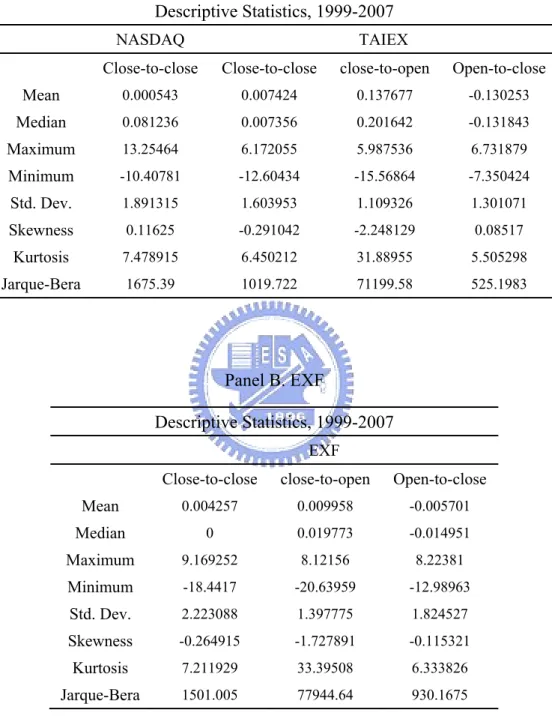
4.3 Descriptive Statistics
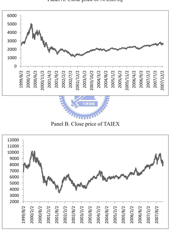
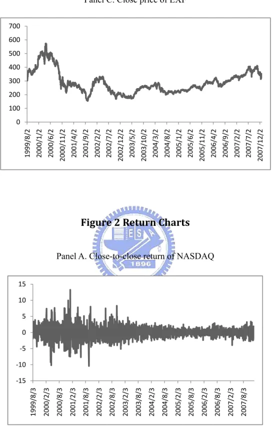
First of all, the historical close price data of NASDAQ, TAIEX and EXF from August 02, 1999 to December 31, 2007 are shown in Figure 1. A quick glance at the charts, we could observe the overall depression after the 911, 2001 attack, and the gradual recovery since 2003. However, the absolute price data contain different scenarios inside; we should take the rate of return into consideration about the further analysis.
< Figure 1 is inserted about here >
The close-to-close, close-to-open and open-to-close returns are computed by the equation (3), (4) and (5) respectively, shown in the Figure 2 below, and whose descriptive statistics are shown in Table 1. The overnight returns (close-to-open return) of TAIEX and EXF accompany the lowest mean value and volatility. The overnight return volatiles with the preceding close price and the is influenced by foreign markets over the no-trading night, and the other returns (close-to-close, open-to-close) both
contain the daily trading hours that might be influenced by all the available information no matter domestic or foreign news. For this reason, the overnight return volatiles with lower variation than the other ones.
< Figure 2 is inserted about here > <Table 1 is inserted about here >
We can also do preliminary analysis for the series from the descriptive statistics; all the series are left-skewed except for close-to-close return of NASDAQ and open-to-close return of TAIEX, because of the negative value of skewness, and all the stock return time series appear to be leptokurtic because the values of kurtosis are larger than 3.
<Table 2 is inserted about here >
Table 2 shows us the simple unconditional correlation between each two series. We can conclude some findings from the simple correlation. First, the close-to-close return of NASDAQ did influence the overnight return (close-to-open return) of TAIEX and EXF, and the correlation coefficients are 0.573 and 0.554 respectively, however, relatively lower correlation exist between NASDAQ and other returns of TAIEX and EXF. It reveals that the foreign market returns did influence the domestic overnight returns more than other types of returns.
4.4 Results of Twostep Estimation
In the two-step estimation, we use the MA(1)-GARCH(1) model to fit the influencing market (NASDAQ) in the first step and the squared term of the resulting residual together with the return are respectively used as explanatory variables in the second step. Our purpose is to model the price changes and volatility spillover effect between the two countries. Table 3 shows us the two-step estimation results of foreign and domestic markets.
<Table 3 is inserted about here >
The estimation model is shown in the description panel of Table 3. As is expected, the time-varying conditional heteroskedasticity is shown by the significant t-statistics of the coefficients of the lagged squared residuals (a1) except for the C2O return of
EXF and the lagged conditional variance terms (a2). The b3 and a4 are coefficients of
price changes and volatility spillover effects respectively. By the estimation results in Table 3, we can conclude some inferences. First of all, the price change spillover effect (coefficient b3) from NASDAQ return to the C2C returns of both TAIEX and EXF is
the largest. It means that among the three types of returns, the C2C returns of TAIEX and EXF were affected by NASDAQ most. The market value of Taiwan Stock Exchange market is about NTD (New Taiwan Dollar) 22 trillion (or U.S. Dollar 0.73
trillion), and the foreign investment institutions have around 34% in hand. Therefore, the foreign funds are very powerful to influence the TAIEX. The foreign investment institutions have a global view of investment, so they will modulate their funds dynamically. Once NASDAQ soars (rises) or plunges (drops), the foreign investment institutions will modulate their foreign (outside the United States) investments to maximize their profits. Taiwan Stock Exchange market is one of the major stock exchange markets in Asia, so the inference of why C2C return of both TAIEX and EXF got the influence from NASDAQ most is possibly from the foreign traders, who adjusted their funds in Taiwan extremely following the performance of the United States stock markets.
Secondly, the C2O returns (overnight returns) of both TAIEX and EXF were also influenced by NASDAQ significantly, however, the volatilities were not. It means that the overnight return of Taiwan stock market was affected by the preceding close price of NASDAQ. Because of no-trading at night, the open price of Taiwan stock market reflects all the available information from the foreign markets, mainly from the United States markets. So it is reasonable to interpret the estimation results of C2O return. However, there were no significant volatility spillover effects from NASDAQ to Taiwan market.
The final inference is about the O2C return. There were significant price change and volatility spillover effects from NASDAQ to TAIEX and EXF, however, the coefficient of price change spillover effect are with a negative sign. The negative coefficients mean that NASDAQ return influenced Taiwan market return in the opposite direction. The result gives us hints that there might be an overreaction on the open price of Taiwan market to the return of NASDAQ. After the overreaction of open price, the market index was adjusted to the proper price within the trading hours. The investors predict the stock price based on all the information set they have, and they reflect their anticipation on the stock prices. Once many investors anticipate the future prices pessimistically or optimistically in the meanwhile, the market might be overreacted. And this is the reasonable interpretation of the negative coefficient of O2C return.
For the weekend effect, the t-statistics of a3 and b1 are insignificant, so the weekend
effect is not obvious to those series. It means that there was no significant difference between the trading days before and after the weekend.
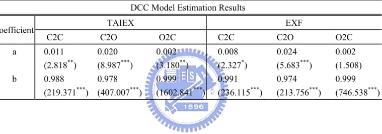
4.5 Results of DCC Model Estimation
This article employed the DCC model to model the correlation with a time-varying covariance between the United States and Taiwan market. Table 4 shows us the results
of DCC model estimation. Except for the coefficient a of O2C return of EXF, all other coefficients a and b of the DCC model estimation are significant and positive.
<Table 4 is inserted about here >
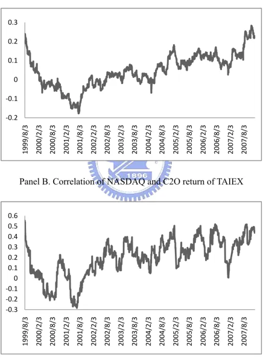
The main purpose of the DCC model estimation is to compute the correlation between two series. The correlation is a numerical data between 0 and 1, and which will tell us the relationship between the two series. Figure 3 shows the correlation results derived from the standard DCC model which was mentioned in chapter 3.
<Figure 3 is inserted about here >
A universal tendency observed in these charts is the upward trend, and which means that the correlation between the respective series was getting stronger and stronger within the empirical time span. We could categorize the patterns of these correlation charts into two types, C2C and C2O returns are the same type, O2C return is the other. The analysis will be started with the first type – for C2C and C2O returns. For C2C and C2O returns, the correlation could be divided into two parts, the former parts were going downwardly, and the later parts were going up. We also can find the critical point occurring in around September 2001 when the 911 attack was taken place. From 1998 to 2001, the dot-com bubble (or called internet bubble) assaulted the United States economy. A huge number of internet companies were
eager to list on NASDAQ to raise fund. The NASDAQ Composite index peaked at 5,048.62 on March 10 2000, but the index was less than 1,700 on September 10 2001. The NASDAQ Composite index plunged about 66% in one and half year. However, the industrial structure of Taiwan stock market is founded on manufacturing, so the direct impact of dot-com bubble from the United States was not serious. So that the correlations of NASDAQ and Taiwan market indexes before 911 attack were going downwardly. After that, owing to the attack, the world economy faced a series of psychological pessimism; investors expected the economy to depress. The linkages among the world markets were getting stronger and stronger. The pessimistic expectation assaulted the markets all over the world, and the impact was really greater than the dot-com bubble. This is the inference that why the correlations were going up after 911 attack. Another point we should take care about is that the correlation got an obvious jump in the second half year of 2007, and that is because the sub-prime mortgage crisis7 erupted in the United States. The subprime crisis is ongoing and
resulting in universal financial problems, attacking not only the stock markets but the
7 The subprime mortgage crisis is an economic problem manifesting itself through liquidity issues in the
banking system, and which is triggered a global financial crisis during 2007 and 2008. The crisis began with the eruption of the US housing bubble and high default rates on subprime and other adjustable rate mortgages (ARM) made to higher-risk borrowers with lower income or lesser credit history than prime borrowers.
banking systems. As a result, it caused the stronger correlation between NASDAQ and Taiwan stock market indexes.
For the O2C returns, the patterns of correlation appear as a line going upwardly. Although the estimated coefficient (a) was not significant for the correlation of NASDAQ and EXF, the pattern of which is very similar to that of NASDAQ and TAIEX. However, the range of the correlation is approximately from -0.15 to +0.1, obviously narrower than that of the first type of pattern correlations, from -0.4 to 0.6. The values of the correlations are negative until after the beginning of year 2005. As the inference in the two-step estimation results in chapter 4.4, the O2C returns of Taiwan indexes overreacted to NASDAQ, and it caused the negative price change spillover effect from NASDAQ to either TAIEX or EXF. It is reasonable to get the negative correlation of C2C return of NASDAQ and O2C return of either TAIEX or EXF. With the linkages among the world markets getting stronger, the correlations are going up slightly with the time, however, the correlations are not so far away from zero (no matter positive or negative), and it implies that the relationships are not very obvious.
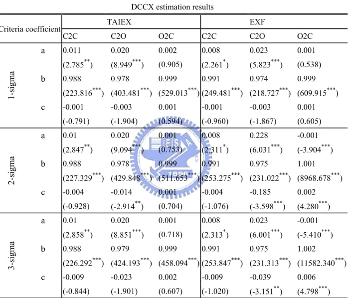
4.6 Results of DCCX Extreme Return Effects
The results are shown in Table 5. There were three scenarios tested by DCCX model, 1-sigma (one time standard deviation away from the mean value of return), 2-sigma, and 3-sigma respectively. The coefficient c stands for the influence of the extreme return occurring in the influencing market (NASDAQ) on the influenced market (Taiwan stock market).
<Table 5 is inserted about here >
By the estimation results of DCCX model, all the coefficients c of the C2C returns of both indexes are insignificant, and it implies that the extreme return effect does not influence either TAIEX or EXF significantly. The results of O2C returns of TAIEX are insignificant as well. However, for C2O returns, almost all the estimation results of coefficient c for these two indexes are significant, and all of them are negative. There are some inferences for the results of C2O returns. When there is an extreme return (no matter 1, 2 or 3 times standard deviation away from the mean value of return) occurring in NASDAQ, the influences on Taiwan indexes are significant and negative. Negative influence means when the extreme return occurs, it will cause the correlation of NASDAQ and either TAIEX or EXF lower. Because there is a price limit constraint of 7 percent away from the previous trading day’s close price in the Taiwan Exchange Index, it will not always reflect the influence from the United States
completely when the extreme return occurs. It is obvious that the incomplete reflection of the NASDAQ impact will lower the correlation between the two markets. Therefore, the significant coefficients c are all negative for C2O returns.
For O2C return of EXF, the result of 1-sigma scenario is not significant but the results of the others are. It implies that for O2C return of EXF, it contains the domestic information available within the trading hours, so when the extreme return is only one time standard deviation away from the mean value of return, the influence on the correlation will be insignificant. However, when the extreme returns are two or three times standard deviation away from the mean, the influence will become significant on the correlation. Furthermore, the influence is positive, and it will enhance the correlation for O2C return of EXF.
5. Conclusion
The United States economy is the most influential one in the world. Especially for the emerging or developing countries' economies, the relationships with the United States' are obviously strong. By the results obtained by this research, we could find that the linkage between Taiwan stock market and NASDAQ is noticeable.
The price changes spillover effects from NASDAQ are all significant to both TAIEX and EXF, and the most significant one is the C2C return, because of the high holding percentage of foreign investment institutions in the Taiwan stock market. There might be an overreaction on the open price of Taiwan market to the return of NASDAQ. After the overreaction of open price, the market index was adjusted to the proper price within the trading hours. The correlations are trending upward after 911-attack in September 2001. The world economies linked more closely after the disaster, and we can see the quantitative evidences from the results of DCC model estimations. By the results of DCCX model estimation, we can conclude that the C2O returns are affected by the extreme returns occurring in NASDAQ most negatively. A strategy of day-trading could be proposed here based on the results found in this research article. We can long (buy) the TAIEX or EXF when NASDAQ plunges (big
drop) and short (sell) when NASDAQ rallies (big rise). The reasons why we trade in this way is that there might be an overreaction occurring in the Taiwan markets, especially when there is an extreme return occurring in NASDAQ. However, within the trading day hours, the domestic information will dominate the foreign information, and then the stock price will converge to the reasonable position. We can observe that by the negative coefficient b3 for O2C return in the two-step estimation results. No matter what investment strategies you use, remember not to lose any of your money. And this is the best policy for investment.
Appendix -
Figures and Tables
Figure 1 Close Price
Panel A. Close price of NASDAQ
Panel B. Close price of TAIEX 0 1000 2000 3000 4000 5000 6000 1999/8/ 2 2000/1/ 2 2000/6/ 2 2000/11 /2 2001/4/ 2 2001/9/ 2 2002/2/ 2 2002/7/ 2 2002/12 /2 2003/5/ 2 2003/10 /2 2004/3/ 2 2004/8/ 2 2005/1/ 2 2005/6/ 2 2005/11 /2 2006/4/ 2 2006/9/ 2 2007/2/ 2 2007/7/ 2 2007/12 /2 2000 3000 4000 5000 6000 7000 8000 9000 10000 11000 12000 1999/8/ 2 2000/2/ 2 2000/8/ 2 2001/2/ 2 2001/8/ 2 2002/2/ 2 2002/8/ 2 2003/2/ 2 2003/8/ 2 2004/2/ 2 2004/8/ 2 2005/2/ 2 2005/8/ 2 2006/2/ 2 2006/8/ 2 2007/2/ 2 2007/8/ 2
Panel C. Close price of EXF
Figure 2 Return Charts
Panel A. Close-to-close return of NASDAQ 0 100 200 300 400 500 600 700 1999/8/ 2 2000/1/ 2 2000/6/ 2 2000/11 /2 2001/4/ 2 2001/9/ 2 2002/2/ 2 2002/7/ 2 2002/12 /2 2003/5/ 2 2003/10 /2 2004/3/ 2 2004/8/ 2 2005/1/ 2 2005/6/ 2 2005/11 /2 2006/4/ 2 2006/9/ 2 2007/2/ 2 2007/7/ 2 2007/12 /2 ‐15 ‐10 ‐5 0 5 10 15 1999/8/ 3 2000/2/ 3 2000/8/ 3 2001/2/ 3 2001/8/ 3 2002/2/ 3 2002/8/ 3 2003/2/ 3 2003/8/ 3 2004/2/ 3 2004/8/ 3 2005/2/ 3 2005/8/ 3 2006/2/ 3 2006/8/ 3 2007/2/ 3 2007/8/ 3
Panel B. Close-to-close return of TAIEX
Panel C. Close-to-open return of TAIEX ‐15 ‐10 ‐5 0 5 10 15 1999/8/ 3 2000/2/ 3 2000/8/ 3 2001/2/ 3 2001/8/ 3 2002/2/ 3 2002/8/ 3 2003/2/ 3 2003/8/ 3 2004/2/ 3 2004/8/ 3 2005/2/ 3 2005/8/ 3 2006/2/ 3 2006/8/ 3 2007/2/ 3 2007/8/ 3 ‐15 ‐10 ‐5 0 5 10 15 1999/8/ 3 2000/2/ 3 2000/8/ 3 2001/2/ 3 2001/8/ 3 2002/2/ 3 2002/8/ 3 2003/2/ 3 2003/8/ 3 2004/2/ 3 2004/8/ 3 2005/2/ 3 2005/8/ 3 2006/2/ 3 2006/8/ 3 2007/2/ 3 2007/8/ 3
Panel D. Open-to-close return of TAIEX
Panel E. Close-to-close return of EXF ‐16 ‐11 ‐6 ‐1 4 9 14 1999/8/ 3 2000/2/ 3 2000/8/ 3 2001/2/ 3 2001/8/ 3 2002/2/ 3 2002/8/ 3 2003/2/ 3 2003/8/ 3 2004/2/ 3 2004/8/ 3 2005/2/ 3 2005/8/ 3 2006/2/ 3 2006/8/ 3 2007/2/ 3 2007/8/ 3 ‐15 ‐10 ‐5 0 5 10 15 1999/8/ 3 2000/2/ 3 2000/8/ 3 2001/2/ 3 2001/8/ 3 2002/2/ 3 2002/8/ 3 2003/2/ 3 2003/8/ 3 2004/2/ 3 2004/8/ 3 2005/2/ 3 2005/8/ 3 2006/2/ 3 2006/8/ 3 2007/2/ 3 2007/8/ 3
Panel F. Close-to-open return of EXF
Panel G. Open-to-close return of EXF ‐15 ‐10 ‐5 0 5 10 15 1999/8/ 3 2000/2/ 3 2000/8/ 3 2001/2/ 3 2001/8/ 3 2002/2/ 3 2002/8/ 3 2003/2/ 3 2003/8/ 3 2004/2/ 3 2004/8/ 3 2005/2/ 3 2005/8/ 3 2006/2/ 3 2006/8/ 3 2007/2/ 3 2007/8/ 3 ‐15 ‐10 ‐5 0 5 10 15 1999/8/ 3 2000/2/ 3 2000/8/ 3 2001/2/ 3 2001/8/ 3 2002/2/ 3 2002/8/ 3 2003/2/ 3 2003/8/ 3 2004/2/ 3 2004/8/ 3 2005/2/ 3 2005/8/ 3 2006/2/ 3 2006/8/ 3 2007/2/ 3 2007/8/ 3
Figure 3 Correlation Charts
This figure shows us the correlation charts with the DCC model. The underlying stocks are NASDAQ with TAIEX and EXF, including the daily C2C, C2O, and O2C returns results.
Panel A. Correlation of NASDAQ and C2C return of TAIEX
Panel B. Correlation of NASDAQ and C2O return of TAIEX ‐0.2 ‐0.1 0 0.1 0.2 0.3 1999/8/ 3 2000/2/ 3 2000/8/ 3 2001/2/ 3 2001/8/ 3 2002/2/ 3 2002/8/ 3 2003/2/ 3 2003/8/ 3 2004/2/ 3 2004/8/ 3 2005/2/ 3 2005/8/ 3 2006/2/ 3 2006/8/ 3 2007/2/ 3 2007/8/ 3 ‐0.3 ‐0.2 ‐0.1 0 0.1 0.2 0.3 0.4 0.5 0.6 1999/8/ 3 2000/2/ 3 2000/8/ 3 2001/2/ 3 2001/8/ 3 2002/2/ 3 2002/8/ 3 2003/2/ 3 2003/8/ 3 2004/2/ 3 2004/8/ 3 2005/2/ 3 2005/8/ 3 2006/2/ 3 2006/8/ 3 2007/2/ 3 2007/8/ 3
Panel C. Correlation of NASDAQ and O2C return of TAIEX
Panel D. Correlation of NASDAQ and C2C return of EXF ‐0.15 ‐0.1 ‐0.05 0 0.05 0.1 0.15 1999/8/ 3 2000/2/ 3 2000/8/ 3 2001/2/ 3 2001/8/ 3 2002/2/ 3 2002/8/ 3 2003/2/ 3 2003/8/ 3 2004/2/ 3 2004/8/ 3 2005/2/ 3 2005/8/ 3 2006/2/ 3 2006/8/ 3 2007/2/ 3 2007/8/ 3 ‐0.2 ‐0.1 0 0.1 0.2 0.3 0.4 1999/8/ 3 2000/2/ 3 2000/8/ 3 2001/2/ 3 2001/8/ 3 2002/2/ 3 2002/8/ 3 2003/2/ 3 2003/8/ 3 2004/2/ 3 2004/8/ 3 2005/2/ 3 2005/8/ 3 2006/2/ 3 2006/8/ 3 2007/2/ 3 2007/8/ 3
Panel E. Correlation of NASDAQ and C2O return of EXF
Panel F. Correlation of NASDAQ and O2C return of EXF ‐0.4 ‐0.2 0 0.2 0.4 0.6 0.8 1999/8/ 3 2000/2/ 3 2000/8/ 3 2001/2/ 3 2001/8/ 3 2002/2/ 3 2002/8/ 3 2003/2/ 3 2003/8/ 3 2004/2/ 3 2004/8/ 3 2005/2/ 3 2005/8/ 3 2006/2/ 3 2006/8/ 3 2007/2/ 3 2007/8/ 3 ‐0.2 ‐0.15 ‐0.1 ‐0.05 0 0.05 0.1 1999/8/ 3 2000/2/ 3 2000/8/ 3 2001/2/ 3 2001/8/ 3 2002/2/ 3 2002/8/ 3 2003/2/ 3 2003/8/ 3 2004/2/ 3 2004/8/ 3 2005/2/ 3 2005/8/ 3 2006/2/ 3 2006/8/ 3 2007/2/ 3 2007/8/ 3
Table 1 Descriptive Statistics
Panel A. NASDAQ and TAIEX Descriptive Statistics, 1999-2007
NASDAQ TAIEX
Close-to-close Close-to-close close-to-open Open-to-close
Mean 0.000543 0.007424 0.137677 -0.130253 Median 0.081236 0.007356 0.201642 -0.131843 Maximum 13.25464 6.172055 5.987536 6.731879 Minimum -10.40781 -12.60434 -15.56864 -7.350424 Std. Dev. 1.891315 1.603953 1.109326 1.301071 Skewness 0.11625 -0.291042 -2.248129 0.08517 Kurtosis 7.478915 6.450212 31.88955 5.505298 Jarque-Bera 1675.39 1019.722 71199.58 525.1983 Panel B. EXF Descriptive Statistics, 1999-2007 EXF
Close-to-close close-to-open Open-to-close
Mean 0.004257 0.009958 -0.005701 Median 0 0.019773 -0.014951 Maximum 9.169252 8.12156 8.22381 Minimum -18.4417 -20.63959 -12.98963 Std. Dev. 2.223088 1.397775 1.824527 Skewness -0.264915 -1.727891 -0.115321 Kurtosis 7.211929 33.39508 6.333826 Jarque-Bera 1501.005 77944.64 930.1675
Table 2 Unconditional Correlation Matrix
Correlation Matrix
NASDAQ TAIEX EXF
Return C2C C2C C2O O2C C2C C2O O2C
NASDAQ C2C 1 0.272 0.573 -0.153 -0.137 0.554 0.235 TAIEX C2C 0.272 1 0.593 0.727 0.685 0.545 0.905 C2O 0.573 0.593 1 -0.122 -0.018 0.864 0.528 O2C -0.153 0.727 -0.122 1 0.860 -0.065 0.665 EXF C2C -0.137 0.685 -0.018 0.860 1 -0.067 0.779 C2O 0.554 0.545 0.864 -0.065 -0.067 1 0.574 O2C 0.235 0.905 0.528 0.665 0.779 0.574 1
Table 3 TwoStep Estimation
Two-Step Estimation Method Using Daily NASDAQ, TAIEX, and EXF
Panel A estimation: h a a e a h a WD Panel B estimation: , h a a e a h a WD a e , Panel C estimation: , h a a e a h a WD a e ,
This table shows us the two-step estimation for the daily return series of NASDAQ, TAIEX and EXF market. Panel A shows us the estimation results for the daily return of NASDAQ. In Panel B, we present the estimation results of the Taiwan Stock Exchange index. Panel C shows us the estimation results of the daily return of EXF. We use MA(1)-GARCH(1,1) model to estimate the coefficients. WDit stands for
weekend dummy variable. Lik fcn is the log likelihood function and the numbers in parentheses are t-statistics values (* indicates significant at 5% level, ** indicates significant at 1% level, and *** indicates significant at 0.1% level).
Panel A: Model estimation for the NASDAQ index Coefficent NASDAQ b0 0.049 (1.572) b1 0.020 (0.291) b2 -0.020 (-0.900) a0 0.006 (0.308) a1 0.054 (5.821***) a2 0.944 (105.216***) a3 0.005 (0.043) lik fcn -3634.062 Skewness -0.116 Kurtosis 3.799 LB-Q(15) 12.542 LB-QS(15) 14.127
Panel B: Model estimation for the TAIEX
Coefficient Close-to-close Close-to-open Open-to-close
b0 0.052 0.229 -0.115 (1.883) (8.100***) (-4.856***) b1 -0.061 -0.044 -0.079 (-0.805) (-0.529) (-1.309) b2 -0.025 0.007 -0.045 (-1.095) (0.086) (-1.938) b3 0.273 0.255 -0.117 (14.047***) (5.263***) (-5.884***) a0 -0.046 0.014 -0.037 (-1.632) (0.473) (-2.252*) a1 0.050 0.268 0.046 (4.958***) (2.424*) (4.857***) a2 0.942 0.731 0.945 (92.163***) (12.998***) (94.069***) a3 0.103 0.183 0.071 (0.736) (1.289) (1.082) a4 0.047 0.023 0.039 (2.817**) (1.168) (3.123**) lik fcn -3463.288 -2711.434 -3097.203 Skewness -0.519 -1.659 -0.148 Kurtosis 6.195 31.535 3.909 LB-Q(15) 12.324 41.217 10.003 LB-QS(15) 13.710 4.290 17.218
Panel C: Model estimation for the EXF
Coefficient Close-to-close Close-to-open Open-to-close
b0 0.065 0.112 0.019 (1.908) (2.224*) (0.629) b1 -0.068 -0.014 -0.128 (-0.636) (-0.197) (-1.467) b2 -0.106 -0.152 -0.062 (-4.661***) (-1.660) (-2.622**) b3 0.352 0.214 -0.124 (12.683***) (2.462*) (-4.528***) a0 -0.101 -0.005 -0.100 (-2.074*) (-0.168) (-3.271**) a1 0.063 0.162 0.065 (4.792***) (1.531) (5.499***) a2 0.927 0.862 0.918 (79.968***) (15.050***) (73.002***) a3 0.302 0.118 0.266 (1.461) (0.961) (2.293*) a4 0.100 0.009 0.103 (2.469*) (0.417) (3.687***) lik fcn -4081.521 -3203.558 -3732.805 Skewness -0.635 -2.797 -0.297 Kurtosis 8.758 72.001 4.571 LB-Q(15) 6.227 45.336 8.676 LB-QS(15) 9.728 1.421 20.522
Table 4 DCC Model Estimation Results The standard DCC model:
q , q ,
q , q , 1 a b q1 q1 a z z , z , z ,
, z , z ,
b qq , q ,
, q ,
This table provides us the estimation results (coefficients a and b) of the standard DCC model employing the daily return of NASDAQ, TAIEX and EXF.
The numbers in parentheses are t-statistics values (* indicates significant at 5% level, ** indicates significant at 1% level, and *** indicates significant at 0.1% level).
DCC Model Estimation Results
coefficient TAIEX EXF
C2C C2O O2C C2C C2O O2C
a 0.011 0.020 0.002 0.008 0.024 0.002
(2.818**) (8.987***) (3.180**) (2.327*) (5.683***) (1.508)
b 0.988 0.978 0.999 0.991 0.974 0.999
Table 5 DCCX Model Estimation Results
This table provides us the estimation results (coefficients a, b and c) of the DCCX model employing the daily rate of return of NASDAQ, TAIEX and EXF.
The numbers in parentheses are t-statistics values (* indicates significant at 5% level, ** indicates significant at 1% level, and *** indicates significant at 0.1% level).
DCCX estimation results
Criteria coefficient TAIEX EXF
C2C C2O O2C C2C C2O O2C
1-sigma a 0.011 0.020 0.002 0.008 0.023 0.001 (2.785**) (8.949***) (0.905) (2.261*) (5.823***) (0.538) b 0.988 0.978 0.999 0.991 0.974 0.999 (223.816***) (403.481***) (529.013***) (249.481***) (218.727***) (609.915***) c -0.001 -0.003 0.001 -0.001 -0.003 0.001 (-0.791) (-1.904) (0.594) (-0.960) (-1.867) (0.605) 2-sigma a 0.01 0.020 0.001 0.008 0.228 -0.001 (2.847**) (9.094***) (0.753) (2.311*) (6.031***) (-3.904***) b 0.988 0.978 0.999 0.991 0.975 1.001 (227.329***) (429.848***) (511.653***) (253.275***) (231.022***) (8968.678***) c -0.004 -0.014 0.001 -0.004 -0.185 0.002 (-0.928) (-2.914**) (0.704) (-1.076) (-3.598***) (4.280***) 3-sigma a 0.01 0.020 0.001 0.008 0.023 -0.001 (2.858**) (8.851***) (0.718) (2.313*) (6.001***) (-5.410***) b 0.988 0.979 0.999 0.991 0.975 1.002 (226.292***) (424.193***) (458.094***) (253.847***) (231.313***) (11582.340***) c -0.009 -0.023 0.002 -0.009 -0.039 0.006 (-0.844) (-1.901) (0.607) (-1.020) (-3.151**) (4.798***)
REFERENCES
Bollerslev, T. I. M., 1990, Modelling the Coherence in Short‐run Nominal Exchange Rates: A Multivariate Generalized ARCH Model, ARCH: Selected Readings 72, 498‐505.
Bollerslev, T. I. M., R. F. Engle, and J. M. Wooldridge, 1995, A Capital‐Asset Pricing Model with Time‐varying Covariances, ARCH: Selected Readings.
Chou, R. Y., J. L. Lin, and C. Wu, 1999, Modeling the Taiwan Stock Market and International Linkages, Pacific Economic Review 4, 305‐320.
Darbar, S. M., and P. Deb, 1997, Co‐movements in international equity markets,
Journal of Financial Research 20, 305‐322.
Engle, R., 2002, Dynamic Conditional Correlation: A Simple Class of Multivariate Generalized Autoregressive Conditional Heteroskedasticity Models, Journal of
Business & Economic Statistics 20, 339‐350.
Engle, R. F., and K. F. Kroner, 1995, Multivariate Simultaneous Generalized Arch,
Econometric Theory 11, 122‐150. Engle, R. F., and K. Sheppard, 2001, Theoretical and Empirical properties of Dynamic Conditional Correlation Multivariate GARCH, (NBER). Grubel, H. G., 1968, Internationally Diversified Portfolios: Welfare Gains and Capital Flows, The American Economic Review 58, 1299‐1314. Liao, Wei‐Yi, 2007, Explaining the Great Decoupling of the Equity‐Bond Linkage with a Modified Dynamic Conditional Correlation Model, Taiwan ETDS. Lo, A. W., and A. C. MacKinlay, 1988, Stock market prices do not follow random walks: evidence from a simple specification test, Review of Financial Studies 1, 41‐66.
Newey, W. K., and D. McFadden, 1994, Large Sample Estimation and Hypothesis Testing, Handbook of Econometrics 4, 2111‐2245.