影像處理與電腦視覺技術應用於駕駛輔助系統之研究

國

立

交

通

大

學

電機與控制工程學系

博 士 論 文

影像處理與電腦視覺技術應用於駕駛輔助系統之研究

A Study of Image Processing and Computer Vision Techniques for

Driving Assistance Systems

研 究 生：林全財

指導教授：吳炳飛 教授

影 像 處 理 與 電 腦 視 覺 技 術 應 用 於 駕 駛 輔 助 系 統 之 研 究

A Study of Image Processing and Computer Vision

Techniques for Driving Assistance Systems

研 究 生：林全財 Student：Chuan-Tsai Lin

指導教授：吳炳飛 Advisor：Prof. Bing-Fei Wu

國 立 交 通 大 學

電機與控制學系

博 士 論 文

A Dissertation

Submitted to Department of Electrical and Control Engineering College of Electrical Engineering

National Chiao Tung University in partial Fulfillment of the Requirements

for the Degree of Doctor of Philosophy

in

Electrical and Control Engineering

June 2009

Hsinchu, Taiwan, Republic of China

iii

影 像 處 理 與 電 腦 視 覺 技 術 應 用 於 駕 駛 輔 助 系 統 之 研 究

研究生：林全財 指導教授：吳炳飛教授

國立交通大學電機與控制工程學系博士班

中文摘要

本論文主要探討應用於駕駛輔助系統之影像處理與電腦視覺技術，包括車道偵測、車 輛偵測、前車距離估測、誤差估測及攝影機動態校正。電腦視覺為基礎(Vision-based)的駕 駛輔助系統利用安裝在智慧車內的攝影機拍攝前方路況，透過車道與車輛偵測技術估測車 道位置、前方車輛與智慧車的距離，這些資訊可以用來提高駕駛安全。本論文主要包含三 個部份，第一部份簡介電腦視覺技術應用於駕駛輔助系統。第二部份為分析偵測道路所得 的資訊及降低誤差的方法，第三部份則提出一些演算法，以應用於估測車輛距離及誤差、 動態校正、以及車道與車輛偵測。 本論文提出一些新的方法來估測前車與智慧車的距離、快速估計前方物件的大小、距 離與物件大小估測結果的誤差分析、及動態校正攝影機參數以降低誤差。首先，利用攝影 機模型將世界座標的地平面座標轉換成影像座標，用以估計前方車輛與攝影機的相對位 置，然後，利用一個新的估計方法估計前車的大小與投射的大小。這個方法利用前方車輛 輪胎與地面的接觸點估計前車與攝影機的距離，並且利用前方車輛的其它頂點之投射位 置，估計車輛的真實大小。因為前車投射的大小會隨著其與攝影機之距離而改變，論文中 提出一個簡單且快速估計投射高度的方法，它能簡化繁複計算及降低計算時間，使得此設 計能應用於即時處理系統。 距離估測的誤差分析結果顯示出當估測車輛與攝影機之間的距離時，攝影機的安裝參 數也會影響到估測的結果，我們藉由誤差分析來找出最合適的攝影機參數以降低誤差。此

外，因為車輛會因路況不平或載重不平衡而晃動或傾斜，安裝在車上的攝影機的外在參數 也會隨著車輛的行進晃動而改變，因此，我們亦提出了動態校正的方法，以取得正確的攝 影機參數，降低估測誤差。實驗結果顯示我們的方法可以準確的估測車輛大小及距離。

論文中也提出了一個快速估測投射的車道與車道線寬度的方法，用以預測車道的可能 位置。另外，設計了一個車道線擷取狀態機 Lane Marking Extraction (LME) Finite State Machine (FSM)，用以辨識影像中的車道線；並將 cubic B-spline 應用於曲線擬合以重建道路 邊界。另外還發展了一個統計搜尋演算法用以決定在不同亮度條件下所設定的車道線擷取 門檻值。此外，有時會有部份車道線被遮蔽而影響偵測，我們應用模糊演算法來判斷車道 線可能被遮蔽的情形，進而利用已有的車道線資訊及估算的車道寬度補償被遮蔽的部份資 訊。最後，為了加速偵測、減少偵測誤差及影像雜訊干擾，亦規劃一個 ROI (Region of Interest) 決定策略，它能提高偵測系統的穩健性並加快偵測速度。 另外，本論文發展了一個以模糊邏輯演算法為基礎的外形大小相似性演算法(Contour Size Similarity, CSS)。利用偵測和估測的影像中車輛大小的比較結果及模糊規則來辨識車 輛。車輛偵測主要針對和智慧車相同車道的前方車輛。實驗結果顯示提出的方法可以有效 的偵測車輛並估計其距離，而且當有車輛切入前方車道時，偵測的目標也會轉移到目前因 切入而成為離智慧車最近的這一輛車。最後章節呈現了本篇論文的結論與未來的研究展望。

v

A Study of Image Processing and Computer Vision

Techniques for Driving Assistance Systems

Student：Chuan-Tsai Lin Advisor：Prof. Bing-Fei Wu

Department of Electrical and Control Engineering

National Chiao Tung University

ABSTRACT

The dissertation aims to explore techniques of image processing and computer vision applicable to driving assistance system, including lane detection, vehicle detection, estimation of the distance to the preceding car, error estimation, and dynamic calibration of cameras. The vision-based driving assistance system films the front road scenes with a camera equipped on the intelligent vehicle, computes lane positions and the distance to the preceding car by the lane and vehicle detection and then adopts the obtained information to improve driving safety. The dissertation mainly includes three sections. The first section is a brief introduction of the application of computer vision techniques to the driving assistance system. The second section presents analyses of the information obtained from lane detection and approaches for reducing errors. The third section proposes some algorithms and their application to the range estimation, error estimation, dynamic calibration, and detection of lanes and vehicles.

The dissertation presents several approaches to estimate the range between the preceding vehicle and the intelligent vehicle, to compute vehicle size and its projective size, and to dynamically calibrate cameras. First, a camera model is developed to transform coordinates from the ground plane onto the image plane to estimate the relative positions between the detected vehicle and the camera. Then, a new estimation method is proposed to estimate the actual and projective size of the preceding vehicle. This method can estimate the range between the preceding vehicle and the camera with the information of the contact points between vehicle tires and the ground and then estimate the actual size of the vehicle according to the positions of its vertexes in the image. Because the projective size of a vehicle varies with its distance to the camera, a simple and rapid method is presented to estimate the vehicle’s projective height, which

allows a reduction of the computation time in the size estimation of the real-time systems.

Errors caused by the application of different camera parameters are also estimated and analyzed in this study. The estimation results are used to determine suitable parameters during camera installation to reduce estimation errors. Finally, to guarantee robustness of the detection system, a new efficient approach of dynamic calibration is presented to obtain accurate camera parameters, even when they are changed by camera vibration arising from on-road driving. Experimental results demonstrate that our approaches can provide accurate and robust estimation of range and size of the target vehicles.

In the dissertation, an approach for rapidly computing the projective lane width is presented to predict the projective lane positions and widths. Lane Marking Extraction (LME) Finite State Machine (FSM) is designed to extract points with features of lane markings in the image and a cubic B-spline is adopted to conduct curve fitting to reconstruct road geometry. A statistical search algorithm is also proposed to correctly and adaptively determine thresholds under various kinds of illumination. Furthermore, parameters of the camera in a moving car may change with vibration, so a dynamic calibration algorithm is applied to calibrate camera parameters and lane widths based on the information of lane projection. Besides, a fuzzy logic is used to discern the situation of occlusion. Finally, an ROI (Region of Interest) determination strategy is developed to narrow the search region and make the detection more robust with respect to the occlusion on the lane markings or complicated changes of curves and road boundaries.

The developed fuzzy-based vehicle detection method, Contour Size Similarity (CSS), performs the comparison between the projective vehicle sizes and the estimated ones by fuzzy logic. The aim of vehicle detection is to detect the closest preceding car in the same lane with the intelligent vehicle. Results of the experiments demonstrate that the proposed approach is effective in vehicle detection. Furthermore, the approach can rapidly adjust to the changes of detection targets when another car cuts in the lane of the intelligent vehicle. Finally, a conclusion and future works are also presented.

vii

誌 謝

終於等到這榮耀的一刻，感覺收獲滿滿，充實自在，辛苦耕耘，含淚收割的果實真是 甜美。回首近六年來的酸甜苦辣，感謝有這些波濤起伏的過程，豐富了我生命的色彩。心 中充滿感謝，感謝很多人的幫助，讓我可以完成這艱鉅的使命。 感謝敬愛的指導教授 吳炳飛教授，嚴謹的教學態度與孜孜不倦的研究精神，啟發我 很多教學及研究的方法，恩師所給的兼具理論與實務的研究方向，使我可以深入探索影像 處理與電腦視覺研究領域的奧秘，進而在這幾年的研究及學習上獲益匪淺。恩師的成長經 歷及奮鬥過程更是學生的榜樣，值得終身學習。 感謝口試委員曾定章教授、張志永教授、賈叢林教授、蘇崇彥教授、陳彥霖教授在論 文口試時的細心斧正與指導，使論文更臻完善。感謝林昇甫教授、張志永教授、鄒應嶼教 授、董蘭榮教授及林一平教授在課業上的教導，使我能順利完成博士班的課業。感謝阿霖 在論文寫作上提供了很多很好的建議，感謝忠哥、暐哥、馬哥、世孟、坤卿、重甫在研究 上，分享了很多的經驗，感謝阿誠、淑閔、秉宗、至明、威儀、正隆及實驗室的學長學弟， 在準備實驗裝備上的協助。感謝和我一起修課的東龍、堯俊、則全、富章、信元、松傑、 學長同學學弟們，一起準備考試、團隊合作完成作業，你們是我的最佳拍檔，我想我會很 懷念在 CSSP 實驗室夜宿苦戰的日子。 感謝碩士班的指導教授劉立頌教授，奠定我理論及研究的基礎。您對學生的關心鼓勵 與親切的教導，也讓我學習到做人處世應有的態度，對事物的看法更為宏觀。 感謝彰化師大附工鍾校長瑞國、劉校長豐旗、與黃校長榮文的鼓勵與對進修的支持， 讓我能有機會持續充實本職學能。 感謝彰化師大附工電子科的老師同仁，瑞祥老師、朝發老師、志洋老師、永安老師、 文漢老師、旺泉老師、文欽老師、建斌老師、志文老師、玉燕老師、明聰老師、及萬金老 師在很多方面的教導與協助；生活上、工作上、專業教學上的經驗分享讓我減少很多獨自 摸索的時間，也讓我的進修學習過程更為順利。感謝勝正、曜忠、天助、泰天、俊宏、冠 宇、豐溢、志偉、信宏、行健、穎俊、勝民、美惠、國隆及這一路相伴的很多學長、同學 與好朋友們，謝謝你們的鼓勵及分享了很多學習上、工作上的寶貴經驗，讓我在無形中增 添了很多智慧，慶幸我有很多好朋友在我的學習歷程中，給我各方面的支援。還有很多曾

經教導我、幫助我、鼓勵我的師長、同仁、朋友，無法一一致意，謹在此表達由衷的感謝， 謝謝您們。 感謝父親母親哥哥姊姊家人們，您們的支持與鼓勵是我的最大動力來源，您們也是我 最有力的後盾。感謝兩個寶貝俞叡與庭陞，你們兩個小調皮總在將家裡搞得天翻地覆的時 候，讓老爸有個鍛練身體運動的機會，你們天真無邪的歡笑聲，也讓我能發現人生的更重 要價值，一切憂愁隨之飄散。感謝摯愛的妻子曉蕙，無論家庭的照料、論文的校稿、甚至 連道路實驗時，擔任實驗車的駕駛助手，都有極高效能的表現，你是最佳賢內助，感謝有 你。 感謝父母、家人、親朋好友們在我遭逢挫折，論文屢次被拒的極度低潮時，對我的支 持鼓勵，讓我雖深陷困厄，仍然從未曾想過放棄，終於能在畢業前能有五篇國際期刊論文 及一個發明專利的成果，謹將這榮耀獻給您們。未來也期許自己能秉持虛心求知的精神持 續學習，在面對人生的各種挑戰上，盡力扮演好自己的角色。 林全財 於 交通大學電機與控制工程學系 CSSP 實驗室 2009/6/1

ix

Contents

摘要...iii

ABSTRACT ...v

誌謝 ...viii

Contents ...ix

List of Figures ...xii

List of Tables ...xv

Chapter 1 Introduction ...1

1.1 Motivation ...1

1.2 Literature Survey ...2

1.2.1 Range Estimation and Dynamic Calibration ...2

1.2.2 Lane Detection ...4

1.2.3 Vehicle Detection ...7

1.3 Research Objectives and Organization of the Thesis ...8

Chapter 2 Range Estimation and Dynamic Calibration ...11

2.1 Introduction ...11

2.2 Position and Size estimation using Projective Geometry ...12

2.2.1 Coordinates transformation Model ...12

2.2.2 Rapid Estimation of Projective Height ...15

2.3 Range and Error Estimation ...19

2.3.1 Digitalized Equation of Range Estimation ...19

2.3.2 Error Estimation ...21

2.3.2.1 Quantization errors ...21

2.3.2.2 Influence of Changes in Translation ...22

2.3.2.4 Influence of Changes in Camera Pan Angles ...24

2.3.2.5 Influence of Changes in Camera Swing Angles ...25

2.4 Dynamic Calibration Method ...27

2.5 Application and Experimental Results ...28

2.5.1 Performance Evaluation on Range Estimation ...29

2.5.2 Simulation Results of Height Estimation ...32

2.5.3 Dynamic Calibration of the Swing Angle ...33

2.5.4 Comparative Performance Evaluation ...34

Chapter 3 Lane Detection ...37

3.1 Introduction ...37

3.2 Camera Model with Dynamic Calibration ...38

3.2.1 Camera Model ...38

3.2.2 Rapid Estimation of the Projective Width ...41

3.2.3 Dynamic Calibration ...42

3.3 Lane Detection ...46

3.3.1 Model of Lane Markings ...46

3.3.2 Lane Marking Extraction ...47

3.3.3 ROI Determination Strategy ...51

3.3.4 Post processing by Fuzzy Reasoning ...59

3.3.5 Reconstruction Process of Occluded lanes ...61

3.3.6 Overall Process of Lane Detection ...64

3.4 Experimental Results ...65

3.4.1 Lane Detection Results ...66

3.4.2 Comparative Performance Evaluation ...81

3.4.3 Comparative Analysis ...89

Chapter 4 Vehicle Detection ...91

xi

4.2 Vehicle Model ...91

4.2.1 Vehicle Features ...92

4.2.2 Adaptive Edge Detection ...94

4.3 Vehicle Detection Based on Contour Size Similarity ...94

4.3.1 Vehicle Detection Procedures ...95

4.3.2 Fuzzy Match ...97

4.3.3 Vehicle Recognition Based on Fuzzy Rules ...100

4.3.4 Vehicle Recognition Based on a Defuzzifier ...100

4.4 Experimental Results ...100

4.4.1 Vehicle Detection Results ...101

4.4.2 Comparative Analysis ...104

Chapter 5 Conclusion and Future Works ...106

5.1 Range Estimation and Dynamic Calibration ...106

5.2 Lane Detection ...106

5.3 Vehicle Detection ...107

5.4 Future works ...108

Appendix A Relation of Projected Width and v-coordinate ...109

Appendix B Adaptation to Illumination Conditions ...111

Reference ...115

Vita ...126

Publication List...127

List of Figures

Figure 1-1. Structure of the thesis...10

Figure 2-1. Coordinate transformation between image plane and ground plane...13

Figure 2-2. The projective geometry of a camera model. (a) A cuboid C. (b) Side

view. (c) Top view...14

Figure 2-3. Relation between M-N image coordinates and u-v image

coordinates………..………...21

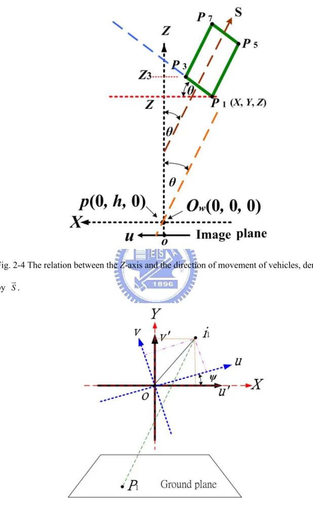
Figure 2-4. The relation between the Z-axis and the direction of movement of

vehicles, denoted by S

ur

...26

Figure 2-5. Relation between the Coordinates (u, v) and (u’, v’)...26

Figure 2-6. Projection of a vehicle and lane markings in the image coordinates....28

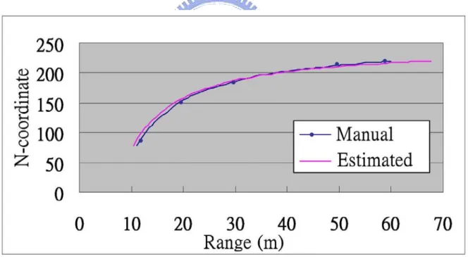
Figure 2-7. A comparison between the manual range measurement and the

estimated range...29

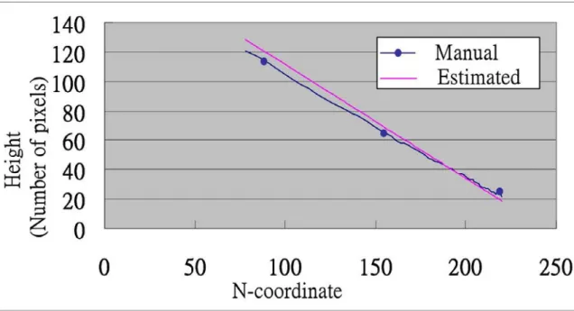
Figure 2-8. A comparison between the manual height measurement and the

estimated height...30

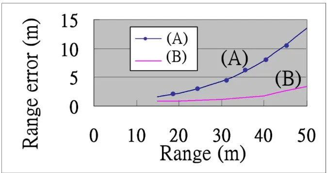
Figure 2-9. A comparison of estimation results between Schoepflin’s approach and

ours...31

Figure 2-10. Estimation of a cuboid’s projective height...32

Figure 2-11. Dynamic calibration of the swing angle...33

Figure 2-12. The swing angle calculated by Liang et al’s and our approaches. (a)

Straight lane markings. (b) The curve of lane markings...36

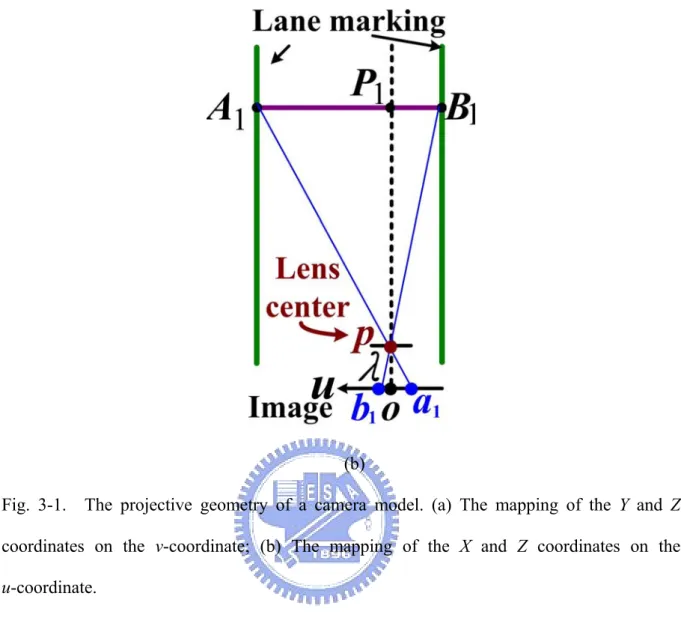
Figure 3-1. The projective geometry of a camera model. (a) The mapping of the Y

and Z coordinates on the v-coordinate; (b) The mapping of the X and Z

coordinates on the u-coordinate...40

Figure 3-2. Relation between w

L

(v) and the v-coordinate...40

xiii

Figure 3-4. Lane Marking Model on a road with lane markings. (a)Actual lane

marking image; (b)The gray level distribution of (a); (c) The gray level

distribution of lane markings in the image coordinates; (d) The variance

of gray level in a row of lane marking...46

Figure 3-5. The lane marking’s relative positions to P

A

and P

B

in different

states...48

Figure 3-6. State diagram of LME FSM...49

Figure 3-7. The flow chart of the selection of ROI determination strategies...51

Figure 3-8. ROI of fixed area...53

Figure 3-9. (a)Bi-directional expansion scheme; (b) Tendency expansion

scheme……….55

Figure 3-10. The acquirement of BFT in a fixed area...56

Figure 3-11. The select of ROI and its range. (a)(b)(c) The application of the

expansion approach; (d) The adoption of the tracking approach...58

Figure 3-12. The B-spline model for lane marking detection...63

Figure 3-13. Procedures of the lane marking detection...64

Figure 3-14. The result of the dynamic calibration of camera’s tilt angle...66

Figure 3-15. The estimated lane width in every frame...67

Figure 3-16. The gray level of lane markings under different illumination. (a)

General light;(b) Strong sunshine; (c)Dusk ; (d) Night...68

Figure 3-17. (a) Curves; (b) A slope; (c)(d) A cloverleaf interchange...72

Figure 3-18. (a)(b)(c)(d)(e)(f) Situations of occlusion with different obstacles...75

Figure 3-19. Results of the nighttime road scene. (a)(b) With road lamps; (c)(d)

Without road lamps...77

Figure 3-20. The detection results under strong sunlight. (a)(b) No occlusion of

vehicles; (c)(d) with the occlusion of a vehicle...79

Figure 3-21. The detection result of a motorcycle inside and outside the lane. (a)

Inside; (b) Outside...80

Figure 3-22. Results of the road scene that the lane markings are occluded with

shadows, signs of braking. (a) Results of Jung and Kelber’s [41]; (b)

Results of the proposed approach...82

Figure 3-23. Results of road scenes with a curve lane and occlusion. (a)Results of

Jung and Kelber’s [41]; (b) Results of the proposed approach...83

Figure 3-24. Results of the road scene under strong sunlight. (a)Results of Jung and

Kelber [41]; (b) Results of the proposed approach...84

Figure 3-25. Results of the nighttime road scene. (a). Results of Jung and Kelber’s

[41]; (b) Results of the proposed approach...86

Figure 3-26. Results of the road scene with a S-shaped lane. (a)(b) Results of Jung

and Kelber’s [41]; (c)(d) Results of the proposed approach...88

Figure 4-1. (a) The projection of an obstacle in the image. (b) The projection of a

pattern in the image. (c) The relation between H

w

and h

i

...93

Figure 4-2. Vehicle detection flowchart...96

Figure 4-3. (a) Size of the obstacle projected on the image. (b) Size of the vehicle

projected on the image...97

Figure 4-4. (a) The membership function of F

h

(b) The membership function of

F

v

...99

Figure 4-5. Vehicle detection with regular illumination...101

Figure 4-6. Vehicle detection with patterns on the road...102

Figure 4-7. Vehicle detection under sunny conditions...102

Figure 4-8. The results of vehicle detection with vehicles cutting in the lane of the

autonomous vehicle...103

Figure 4-9. Results of lane and vehicle detection. ...104

Figure B-1. The gray level distribution with a row of lane marking in the search

window...111

xv

List of Tables

Table 2-1 Relations between N and Z coordinates...19

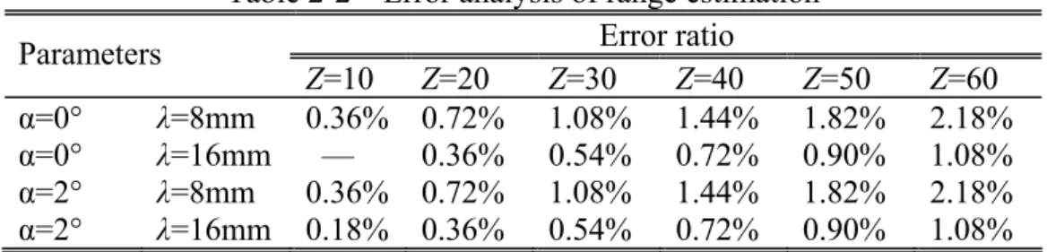
Table 2-2 Error analysis of range estimation...20

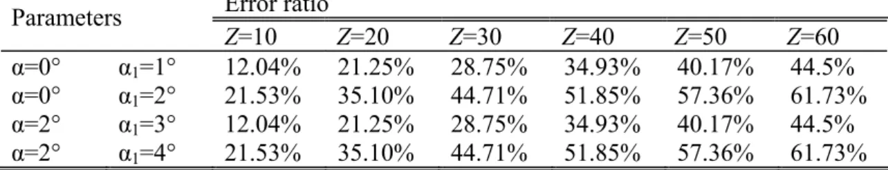
Table 2-3 Error analysis of range estimation caused by change of tilt angles ...22

Table 2-4 Variation ratio between P

1

and P

3

on the Z-coordinate...24

Table 2-5 Variations between (u, v) and (u’, v’)...25

Table 2-6 Experimental results of camera angle estimation...31

Table 2-7 Comparison of Approaches...35

Table 2-8 A comparison in estimation results of camera angle and errors...35

Table 3-1 Denotations of the five G

d

conditions...50

Table 3-2 The computation timings under different conditions by the proposed

system...…66

Table 3-3 Results of lane width estimation in the four situations...69

Table 3-4 The obtained parameters under different illumination conditions……...70

Table 3-5 Comparison of different algorithms...90

Chapter 1

Introduction

1.1 Motivation

Driving assistance systems have become an active research area in recent years for developing intelligent transportation systems (ITS). On average, there is at least one man dying of vehicle crash every minute and more than 10 million people getting injured in the auto accidents, 2 or 3 million of whom are seriously wounded. Therefore, researches concerning crash avoidance, the reduction of injury and accidents, and the manufacture of safer vehicles are very important. Vehicle accident statistics reveal that the greatest threat to a driver comes from other vehicles. Accordingly, the objective of automatic driving assistance systems is to provide drivers with the information with respect to the surrounding traffic environment to lower the possibility of collision [1]-[3].

Currently, various sensors have been applied to driving assistance systems. Driving assistance systems require information regarding lanes, the preceding vehicle and its range to the intelligent vehicle. Lane detection usually entails vision-based techniques, which require the use of single cameras or stereo cameras. Approaches to vehicle detection and range estimation are multiple. Besides vision-based techniques, laser sensors are often adopted. If a system involves several or many kinds of sensors, the cost will rise and the complexity of the system will increase. By contrast, the use of only a single camera can significantly reduce the cost.

the camera can affect the results of range estimation; however, the parameters are easily changed by the vibration caused by the vehicle movements. Therefore, setting parameters correctly to reduce errors and dynamic camera calibration are necessary issues for researches. Besides, vehicles often move rapidly so driving assistance systems should be able to promptly respond to results of lane and vehicle detection to avoid the occurrence of traffic accidents. Hence, the acceleration of detection is also a major research issue. Furthermore, adaptive lane and vehicle detection systems are required to cope with changes of weather and illumination in the outdoor environment. Accordingly, the objective of this study is to develop methodologies for adaptive and real-time driving assistance systems [4]-[8].

1.2 Literature Survey

1.2.1 Range Estimation and Dynamic Calibration

Previous studies often adopted laser, radar or computer vision techniques in range estimation issues. For example, Chen [9] presented a radar-based detector to find obstacles in the forward collision warning system, where a vision-based module was adopted to confirm that the detected object is not an overhead structure to avoid false alarms of the warning system. Segawa et al. [10] developed a preceding vehicle detection system for collision avoidance by using a combination of stereo images and non-scanning millimeter-wave radar. In Hautiere et al.’s method [11], a depth map of the road environment is computed and applied for detecting the vertical objects on the road. Stereo-vision based techniques can also be applied on range estimation. By comparing the disparities of two images, obstacles can be detected and their distance to the experimental vehicle can also be estimated [11][12]. However, the methods above need multiple cameras or at least one set of radar to detect obstacles and estimate the range. If only one single camera is required, the cost and the complexity of the system will be significantly decreased. Nevertheless, the estimation results

of a single camera are often influenced by external camera parameters and thus serious errors arise. For example, an outdoor camera is often affected by the wind or rain. Furthermore, camera parameters vary with the pressure of tires, unbalanced load or bumpy roads when the camera is mounted on a moving vehicle. Therefore, automatic calibration is necessary to deal with the above issues. Studies of camera calibration usually adopted points in the world coordinates or certain distinctive patterns [13]-[15]. For instance, Wang and Tsai [13] proposed a camera calibration approach using a planar hexagon pattern drawn on the ground. However, this approach may only be suitable for calibration of fixed cameras. Schoepflin and Dailey [14] supposed the camera swing angle was zero and searched for the vanishing point by extending lane markings in the image to calibrate the tilt angle. Nevertheless, when the camera swing angle is not zero, errors may arise. Liang, et al. [15] calibrated the tilt angle of a moving camera with the coordinate of the vanishing point. However, the assumption of vehicles staying in the center of lanes may not be reasonable under typical driving conditions and thus such methods may cause more errors on roads with curves. Therefore, it is better if calibration targets are objects available on the road and errors caused by incomplete assumptions should be estimated. In fact, camera intrinsic parameters are usually fixed while extrinsic parameters such as angles and heights are variable. Intrinsic parameters can be obtained by analyzing a sequence of images captured by cameras [16]-[19]. To solve the problem of changing extrinsic parameters, we propose an approach of automatic calibration to provide robust range estimation for vision-based systems.

Object features, like sizes and shapes, are widely employed in the recognition of objects [20]-[25]. Yilmaz et al.[20] adopted a method of contour-based object tracking to detect pedestrians and to solve the problem of occlusion between objects. Lin et al.[21] computed the number of people in crowded scenes by detecting features of human heads. Pang et al.[22] analyzed vehicle projections with geometry and divided their occlusions in the images to

provide essential information to the traffic surveillance systems. Broggi et al.[23] utilized inverse perspective mapping to transfer images of the front driving lanes into a bird’s view of parallel lanes to detect and identify vehicles with a bounding box. However, most of the above-mentioned approaches may need the prior information about the projective size and shape of the target object, and it may not be possible to obtain this information accurately and rapidly in many situations. Moreover, the loss of dimensional information during the transformation from 3-D coordinates to 2-D image coordinates often increases difficulties in estimating the projective size and shape of the target object. To solve the problem, we regard a vehicle as a cuboid and with the world coordinates of the cuboid’s vertex on the ground, we can estimate the world coordinates of other vertices in the cuboid, determine their projective positions and estimate the size of the cuboid. Since vehicle sizes are within certain ranges, cuboids on the drive lanes whose sizes fit general vehicle sizes should be vehicles. So our method can be applied to vehicle recognition.

1.2.2 Lane Detection

There are many ways lane detection can be achieved. In early studies, Dickmanns et al. [26]-[28] conducted 3-D road recognition by adopting horizontal and vertical mapping models, the approach of extracting features with edge elements, and recursive estimation techniques. The results were applied to their test vehicle (VaMoRs) to function as autonomous vehicle guidance. Broggi et al. [29][30] used IPM (Inverse Perspective Mapping ) to transfer a 3-D world coordinate to a 2-D image coordinate, and detected road markings using top-view images. Kreucher and Lakshmanan [31] suggested detecting lane markings with frequency domain features that capture relevant information about edge-oriented features. The objectives of many studies on lane detection include autonomous vehicle guidance and driving assistance such as lane-departure-warning and Driver-Attention Monitoring systems. Some

assumptions in common are as follows: 1) The road is flat or follows a precise model. 2) The appearance of lane markings follows strict rules. 3) The road texture is consistent. The main difficulty in lane detection is how to recognize roads efficiently in various situations, including complex shadowing and changes in illumination [32][33]. Furthermore, the vibration of a moving camera causes changes in camera parameters and thus leads to errors in geometric transformation. To solve the problem, dynamic calibration of cameras is required to improve robustness [34]-[36].

The task of lane detection can be summarized as two main sections: 1) The acquirement of features. 2) A road model for reconstructing road geometry. In addition, to accelerate the detection and make it robust, some approaches are added such as narrowing the search region, the determination of ROI (Region of Interest), dynamic calibration for the camera and position-tracking methods using consecutive images.

The first step of detecting lanes is to extract their features. On most occasions there are lane markings on both the left and the right side of the driving lane, while sometimes only the boundaries of the road exist without any lane marking. Most parts of the lane markings are like two parallel ribbons with some variations, for example, being straight or curved, solid lines or dashed lines, and in the color of white, yellow or red. The occlusion of trees and buildings and their shadows makes it more difficult to detect positions of lanes. Also, visibility varying with illumination increases difficulty to detections [37]-[41].

In acquiring features, there are four major types of methods: pixel-based, edge detection-based, marking-based, and color-based methods. The pixel-based type is to classify pixels into certain domains and put pixels of the road boundaries in one category [42]-[44]. The edge detection-based type involves conducting edge detection in the image first. Then, find straight lines with Hough transform [45][46] or adopt an ant-based approach to start a bottom-up search for possible path of the road boundary in the image [47]-[50] or determine

search regions by road models for detection of road boundaries [1][51]-[53]. Those two methods are time-consuming, and easily cause errors when complex shadows or obstacle occlusion exist. The marking-based type is based on features of lane markings. For example, Bertozzi and Broggi [29] proposed IPM and black-white-black transitions to detect lane markings. This method may effectively deal with some situations of shadows or obstacle occlusions. However, the vibration caused by the moving vehicle may influence the extrinsic parameters of the camera, and thus arouse unexpected mapping distortions on images, which may cause errors on lane detection results. The color-based type is to utilize color information of the road in the image [44][54]-[56]. In this way, there is more information about the lane and better abilities to resist noise. However, it takes more computation time to extract color features of interest.

Since shadows of trees or other noises usually exist and some lane markings are dash lines, the detected features of road boundaries are often incomplete. Therefore, the methods of interpolation or curve fitting are needed to reconstruct the road geometry. Kreucher and Lakshmanan [31] used a deformable template shape model to detect lanes. They believed that two sides of a road respectively approximate a quadratic equation, so they established their coefficients to determine the curvature and orientation of the road. However, curve fitting cannot be done by a quadratic equation on the lanes with S-shaped turns. So Wang et al. [57] adopted spline interpolation which can be used in various curves to connect line segments. However, when there are vehicles in the lane occluding parts of the lane boundary, some errors may arise, because this approach found a vanishing point depending on Hough transform followed by line-length voting. Thus, vehicles on the lanes may form spurious lines which may influence the determination of the vanishing line. Furthermore, Hough transform and Canny edge detector utilized in Wang et al.’s approaches may take more computation time.

Another issue to promote lane detection efficiency and depress noise sensitivity is to set appropriate ROI. Lin et al.[58] applied the information of both lane boundaries obtained from initial detection in the first frame to the finding of ROI on Hough domain. Then ROI was adopted as search parameters of lane boundaries in the subsequent frames. The method can effectively accelerate lane detection process on a straight lane but errors may arise on road curves. Chapuis et al.’s method [59] utilized an initially determined ROI to recursively recognize a probabilistic model to conduct iterative computation, and adopted a training phase to define the best interesting zone. The initially set ROI is effective in the general roads; however, diverse road curves may make the initial ROI too large on the farther part of the road and thus raise noise sensitivity. Therefore, an effective method is needed for adaptive determination of ROI and adjustment to changes of road curves in the image sequences, and thus ROI can be significantly narrowed to obtain more accurate and faster lane detection results.

1.2.3 Vehicle Detection

Besides lane detection, detections of obstacles and vehicles are also important issues in the research of crash avoidance and vehicle following. Some investigations exploited stereo visual systems to detect obstacles by comparing differences between two images [60][61]. Two cameras were required by those approaches, and thus the cost increased. In some previous studies, an obstacle was recognized as a vehicle by its shape and symmetry [12][62]-[64]. Practically, features of the vehicles presented in the images are also helpful to the detection. Sun et al. analyzed features of vehicles in the images, segmented and recognized vehicles with a Gabor filter and neural network techniques. In their study, the possible positions of vehicles were checked with hypothesis generation (HG) first and then the presence of the vehicles was verified by hypothesis verification (HV) [65][66]. Some

researchers performed optical flow analysis to detect obstacles. In consecutive images, positions of an object only have slight changes. Therefore, in the subsequent images, an object is found by the prediction of its motion based on its previous position [67]-[69]. Still, some problems may increase the detection time and make it difficult to achieve real-time vehicle detection. For example, the range between the camera and a recognizable vehicle is about 5-60m. The size of the vehicle in the range of 5m has changed enormously from that in the 60m. Besides, the diversity of vehicle colors, shapes, and sizes complicates the design of classifiers in vehicle recognition. Therefore, to detect vehicles rapidly, the feature of a rectangle-like contour in most vehicles should be adopted and the problem that projective sizes of vehicles vary with their range to the camera should be taken into consideration.

In vehicle detection, an approach of geometry transformation is proposed to estimate the projective sizes of vehicles. Furthermore, Contour Size Similarity (CSS) approach is presented to discover vehicles that threaten driving safety. With only one single camera applied, the cost of CSS is far less than that of a stereo vision approach. Furthermore, the search area of the vehicle detection can be narrowed based on results of lane detection, because only the closest preceding car in the lane of the autonomous vehicle is interested. Once the closest car is detected, the approach of vehicle detection starts to compute its range to the camera [70][71]. When another vehicle cuts in, the approach can also shift its detection target immediately.

1.3 Research Objectives and Organization of the Thesis

The objective of this dissertation is to develop advanced vision-based methodologies for driving assistance systems. The developed approaches consist of range and size estimation, error analysis of the estimated results, dynamic camera calibration, lane model, lane detection, the approach of Contour Size Similarity, and vehicle detection. For driving assistance systems,

information concerning the positions of lanes and the preceding vehicles are important. In the study, a camera model is first adopted to estimate the actual and the projective sizes of the detected targets and approaches to reduce detection errors and accelerate detection are also developed. Then, lane positions in the images are extracted by Lane Marking Extraction (LME) Finite State Machine (FSM) based on information of properties of lane markings. B-spline is also used to reconstruct road boundaries. Afterwards, the approach of contour size similarity is presented to detect vehicles within the driving lane and estimate their range to the camera. The obtained information is applied to driving assistance systems to improve driving safety.

The material in dissertation is organized according to the approaches used in driving assistance systems. A simplified overview is shown in Fig. 1-1. In Chapter 2, the dissertation presents new approaches to estimate the range between the preceding vehicle and the intelligent vehicle, to estimate vehicle size and its projective size, and to dynamically calibrate cameras. A lane model is presented in Chapter 3. For lane detection, a LME FSM is designed to extract lane markings with a lane model. Then, the obtained lane boundaries can be applied to determine the search region of vehicle detection. In Chapter 4, the developed fuzzy-based vehicle detection method, Contour Size Similarity (CSS), performs the comparison between the projective vehicle sizes and the estimated ones to recognize the target vehicle by fuzzy logic. The target of vehicle detection is the closest preceding car in the same lane with the intelligent vehicle. The experimental results demonstrate that our approaches effectively detect vehicles under different situations.

Chapter 2

Range Estimation and Dynamic

Calibration

2.1 Introduction

Accurate and real-time detection of vehicle position, speed and traffic flows are important issues for driving assistance systems and traffic surveillance systems [1][72]-[74]. During the detection, errors often arise because of camera vibration and constraints such as the limitations of image resolution, quantization errors, and lens distortions [34][75]. Therefore, accurate error estimation is important in vehicle detection issues, and image processing techniques for position estimation or motion detection are necessary in many situations [7][76]-[78]. However, most of the previous studies have not involved methods of reducing errors caused by changes of camera parameters, while some important issues like error estimation and the way to set appropriate camera parameters were seldom considered. This may influence the determination of camera parameters and the specifications of a detection system. Therefore, we propose an effective strategy to reduce errors of range estimation by determining the most suitable camera parameters.

In this study, we apply error estimation to determine proper camera parameters and then estimate actual and projective sizes of target objects to facilitate vehicle recognition. An approach to rapidly compute projective sizes is also proposed to significantly reduce the computational cost of vehicle detection process for real-time and embedded systems. Then, a

dynamic calibration approach is presented to calibrate the tilt and swing angles of the camera with information of lane markings and vehicles in the image. The experimental results demonstrate that our work can provide accurate and robust range and size estimation of target vehicles. The rest of this chapter is organized as follows: Section 2.2 presents position and size estimation using projective geometry. Section 2.3 explores range estimation and error estimation with various camera parameters. Section 2.4 proposes a dynamic calibration approach to deal with the problem of camera vibration and variation in camera angle. Section 2.5 displays experimental results of range and height estimation, dynamic calibration of camera angles, and comparisons with other approaches.

2.2 Position and Size estimation using Projective Geometry

The position of any point in the 3-D world coordinates (X, Y, Z) projected to a 2-D image plane (x, y) can be calculated through perspective transformation [13]. Mapping a 3-D scene onto the 2-D image plane is a many-to-one transformation. However, mapping a point on the front horizon of the camera onto an image plane is a one-to-one transformation. Therefore, the relative position between the camera and any point on the ground can be estimated by the coordinate transformation between image plane and ground plane.

2.2.1 Coordinates Transformation Model

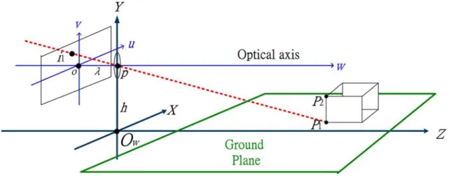
Figure 2-1 shows the coordinate transformation between image plane and ground plane, where Ow denotes the origin of the world coordinates (X, Y, Z), and O represents the origin of

the image coordinates (u, v). Let λ be the focal length of the camera; p denote the lens center;

h represent the height. As shown in Fig.2-2(a), there is a cuboid C associated with a target

object, whose lengths, widths and heights are L1, W1, and H1, respectively. Let P1(X, 0, Z) be

inferred from the size of C. Other vertices can be estimated in the same way. Based on the cuboid’s size and the position of its vertex, P1, the projective positions of other vertices in a

cuboid can be estimated to accurately estimate the contour and size of the cuboid’s projection.

Fig. 2-1. Coordinate transformation between image plane and ground plane.

Figure 2-2(b)(c) presents the side view and top view of the image formation. In the figure, tilt angle α denotes the angle between the Z-axis and the optical axis, pE. P1(X, 0, Z) projects

onto i1(u, v) on the image plane, and the transformation between the two coordinates can be

expressed as (2.1) and (2.2) by applying trigonometric function properties and our previous study [34], where ||Z|| and ||X|| respectively denote the range and lateral position between P1

and the camera.

1 ( ) tan - tan 2 v Z v _{= ⋅}h ⎛⎛ ⎞₋ − ⎛ ⎞⎞ ⎜ ⎟ ⎜ ⎟ ⎜_{⎝ ⎠ ⎝ ⎠}⎟ ⎝ ⎠ π α λ (2.1) 1 ( , ) tan - tan 2 u v X u v _{= − × ⋅}h ⎛⎛ ⎞₋ − ⎛ ⎞⎞ ⎜ ⎟ ⎜ ⎟ ⎜_{⎝ ⎠ ⎝ ⎠}⎟ ⎝ ⎠ π α λ λ (2.2)

(a)

(b)

(c)

Fig. 2-2. The projective geometry of a camera model. (a) A cuboid C. (b) Side view. (c) Top view.

Let P2 and P3 respectively project onto i2(u2, v2) and i3(u3, v3). The PP is the height of 1 2

cuboid C, whose projective height is hi12 in (2.3). The distance between P1 and P3 is the width

of C ; its projective width is wi13 in (2.4).

Based on (2.1)-( 2.4), if P1 of the cuboid can be found in the image, then the position and

size of the cuboid can be estimated. Likewise, the relation between v2 and H1 can be obtained

by (2.3), as shown as (2.5). Further by applying (2.5), we can have the height of the cuboid C as in (2.6). 12 2 i h = − , (2.3) v v where

_{( )}

1 tan 2 v Z h − ⎡⎛ ⎞ ⎛ ⎞⎤ = × _⎢⎜ − _⎟− _{⎜ ⎟⎥} ⎝ ⎠ ⎝ ⎠ ⎣ ⎦ π Z λ tan α ,

( )

1 2 1 tan 2 v Z h H − ⎡⎛ ⎞ ⎛ ⎞⎤ = × _⎢⎜ − _⎟− _{⎜ ⎟⎥} − ⎝ ⎠ _{⎝ ⎠} ⎣ ⎦ π Z λ tan α 13 1 i w W Z = ×λ (2.4) 1 2 1 tan 2 1 tan 2 h H v h H ⎧ _{⎛ ⎞} ⎛ ⎞ ⎫ − − ⎪ ⎜_⎝ ⎟_⎠ ⎜ ₋ ⎟ ⎪ ⎪ ⎝ ⎠ ⎪ = λ ⋅ ⎨ _{⎛ ⎞}⎬ ⎛ ⎞ ⎪ _{+ ⎜ − ⎟×⎜ ⎟}⎪ ⎪ ⎝ _{⎠ ⎝} − ⎠⎪ ⎩ ⎭ π Z α π Z α (2.5) 2 1 2 tan 2 tan 2 _tan 2 v h H h Z v ⎛ _⋅⎛ _⋅ ⎛ ₋ ⎞₋ ⎞⎞⎛ ⎞ ⎜ _{⎛ ⎞} ⎜_⎝ ⎜_⎝ ⎟_⎠ ⎟ ⎜_⎠⎟ ⎟ ⎜ ⎟⎜ ⎟ = ⋅ _⎜ − _⎟− − ⎜ ⎝ ⎠ ⎟⎜ _⋅ ⎛_{⎜ −} ⎞_⎟ ⎟ ⎜ ⎟ ⎜ ⎟_{⎝ ⎝ ⎠ ⎠} ⎝ ⎠ π Z α π λ α π λ _{λ α} (2.6)

2.2.2 Rapid Estimation of Projective Height

A cuboid’s projective size varies with its relative position with the camera. From (2.3), we can estimate its projective height. When applied to driving assistance, the rapid size estimation of the front vehicle’s projection can provide helpful information for vehicle recognition and determination of vehicle size.

( )

tan 2 tan 2 h Z v Z h Z ⎧ _⋅ ⎛ ₋ ⎞₋ ⎫ ⎜ ⎟ ⎪ ⎪ ⎪ ⎝ ⎠ ⎪ = ⎨ _{⎛ ⎞}⎬ ⎪ _{+ ⋅ ⎜ − ⎟}⎪ ⎪ ⎝ ⎠⎪ ⎩ ⎭ π α λ π α (2.7)

From (2.1), we can obtain the relation between Z and v as shown in (2.7). In Fig. 2-2 (b),

there is an object whose height is H1. Therefore, supposing that P1(X, 0, Z) projects onto i1(u,

v), we can re-write (2.3) to turn hi12(v) into a linear equation shown in (2.8). Since the camera

is mounted on an experimental vehicle for object detection, when α is too large, the farther

part of the lane will not appear in the image. Therefore, α is usually between 0-6 degrees. Also, the height of the camera is restricted by the height of the vehicle roof, to be lower than 1.5 meters. Furthermore, the range Z of the preceding vehicle is usually over 10m, and thus

we can obtain (2.9) and (2.10). Then, substitute (2.9) and (2.10) into (2.8) to get (2.11). Also, by substituting (2.1) into (2.11), we obtain hi12(v) as shown in (2.12). Equation (2.13) means

the first derivative for v to hi12(v). Let ξ = (π/2- α), and τ = tan-1(v/λ). (2.15), (2.16) and (2.17)

derive from (2.13) and (2.14). In this study, let α<6°, so ξ>84°, to get (2.18) and (2.19). Then they are substituted to (2.17) to obtain (2.20) and (2.21). (2.21) shows the first derivative of hi12(v) is a constant. Therefore, the relation between the projective height of

1 2

PP , hi12(v), and the projected v-coordinate of P1 can be expressed by a linear equation as

(2.22).

( )

1 12 1 tan ( ) tan 2 2 tan ( ) tan 2 2 i h Z h H Z h v h Z h H Z ⎧ _⋅ ⎛ ₋ ⎞_{− − ⋅} ⎛ ₋ ⎞₋ ⎫ ⎜ ⎟ ⎜ ⎟ ⎪ ⎪ ⎪ ⎝ ⎠ ⎝ ⎠ ⎪ = _⎨ − _⎬ ⎛ ⎞ ⎛ ⎞ ⎪ _{+ ⋅ ⎜ − ⎟ − + ⋅ ⎜ − ⎟}⎪ ⎪ ⎝ ⎠ ⎝ ⎠⎪ ⎩ ⎭ π π α α λ π π α α (2.8) tan tan 2 2 h Z+ ⋅ ⎛_⎜ − ⎞_⎟≅ ⋅Z ⎛_⎜ − ⎞_⎟ ⎝ ⎠ ⎝ ⎠ π π α α (2.9) where h<1.5, α < 6°, Z > 10.

1 ( ) tan tan 2 2 h H− + ⋅Z ⎛_⎜ − ⎞_⎟≅ ⋅Z ⎛_⎜ − ⎞_⎟ ⎝ ⎠ ⎝ ⎠ π π α α (2.10) where H1 < 2.

( )

1 12 i H h v Z × ≅ λ (2.11)

( )

1 12 1 tan - tan 2 i H h v v h − × ≅ ⎛⎛ ⎞ ⎛ ⎞⎞ ⋅ _{⎜⎜ ⎟}− _{⎜ ⎟⎟} ⎝ ⎠ ⎝ ⎠ ⎝ ⎠ λ π α λ (2.12)

( )

1 12 1 cot - tan 2 i v d dh v H dv h dv − ⎛⎛ ⎞₋ ⎛ ⎞⎞ ⎜ ⎟ ⎜ ⎟ ⎜ ⎟ × ⎝⎝ ⎠ ⎝ ⎠⎠ ≅ × π α λ λ (2.13)

(

)

1 tan

_{( )}

( )

tan

_{( )}

( )

cot tan tan + ξ × τ ξ − τ = ξ − τ (2.14)

( )

( )

( )

(

)

12 1 1 2 2 tan tan i d d dh v H f f dv h − × ≅ × ξ − τ λ (2.15) where 1

(

( )

( )

)

(

( )

( )

)

1 tan tan tan tan d d f dv + ξ × τ = ξ − τ × ,

( )

( )

(

)

(

( )

( )

)

2 tan tan 1 tan tan d d f dv ξ − τ = + ξ × τ × .

( )

( )

( )

( )

( )

( )

1 2 1 2 1 ta n ta n ta n 1 ta n ta n i d h v d v v v d d v v H d v d v h v ≅ ⎛ _{+ ξ ×} ⎞ ⎛ _{ξ −} ⎞ ⎜ ⎟ ⎜ ⎟ ⎛ _{ξ −} ⎞_× ⎝ ⎠ ₋⎛ _{+ ξ ×} ⎞_× ⎝ ⎠ ⎜ ⎟ ⎜ ⎟ × _{× ⎝ ⎠ ⎝ ⎠} ⎛ _{ξ −} ⎞ ⎜ ⎟ ⎝ ⎠ λ λ λ λ λ λ (2.16) ( ) ( ) ( ) ( ) ( ) 12 1 2 tan 1 tan 1 tan tan i v v dh v H dv h v ξ ⎛ _{ξ −} ⎞_{× − +}⎛ _{ξ ×} ⎞ ⎛_{× −} ⎞ ⎜ ⎟ ⎜ ⎟ ⎜ ⎟ × _{⎝ ⎠ ⎝ ⎠ ⎝ ⎠} ≅ × ⎛ _{ξ −} ⎞ ⎜ ⎟ ⎝ ⎠ λ λ λ λ λ λ (2.17)

( )

tan ξ >>v λ (2.18) where ξ > 84°.

( )

tan

( )

( )

1 tan ξ × ξ >>⎛_⎜ v ×tan ξ + ⎞_⎟ ⎝ 2 ⎠ λ λ λ (2.19)

( )

( )

( )

( )

(

)

12 1 2 tan tan tan i dh v H dv h ξ ξ × × ≅ × ξ λ _λ (2.20)

( )

12 1 i dh v H dv ≅ h (2.21)

( )

1 12 1 i H h v v C h ≅ × + (2.22) where C1 is a constant.

From the sequential images, we get the actual projective height of PP_{1 2}. Let the projective

height of P P_{1 2} be hi12(va) when P1 projects onto va, and the height be hi12(vb) when projecting

onto vb. Then, by substituting the obtained hi12(va) and hi12(vb) into (2.22), C1 and H1 can be

obtained as expressed in (2.23) and (2.24).

( )

( )

(

)

12 12 1 i a i b a b h h v h v H v v ⋅⎡_⎣ − ⎤_⎦ ≅ − (2.23)

( )

1 1 i12 a a H C h v v h ≅ − × (2.24) By comparing (2.3) and (2.22), we can find that the proposed approach of projective height estimation significantly reduces the computation cost. Also, the comparison between (2.6) and (2.23) shows that the proposed approach requires much less computation timing for estimating the actual height of the target object.

2.3 Range and Error Estimation

Inaccurate camera parameters often cause estimation errors. Even if the parameters are initially set accurately, they could be changed by external forces, or by the use of mechanical devices, causing the estimated value to be different from the real value. The range estimation results are discussed below.

2.3.1 Digitalized Equation of Range Estimation

To estimate range with a single camera, the equation evolved by the camera model should be digitalized first. Therefore, an affine transformation from real image coordinates (u, v) to bitmap image coordinates (M, N) can be obtained by (2.25). Figure 2-3 displays the relationship between the M-N bitmap image coordinates and the u-v real image coordinates, where the left bottom images denotes the origin Q(0, 0).

1 _{/ 2,} 1 _{/ 2,}

x m y n

M = −d− × +u M = −N d− × +v N (2.25) where dx and dy are respectively horizontal and vertical physical distances between adjacent

pixels, and the frame size is Mm by Nn pixels.

Table 2-1 Relations between N and Z coordinates

The units of N and Z are the numbers of pixels and meters respectively. Z-coordinate (Meter) Parameters N=0 N=100 N=200 N=300 N=400 N=492 α=0° λ=8mm 5.715 9.63 30.56 ∞ ∞ ∞ α=0° λ=16mm 11.43 19.25 61.11 ∞ ∞ ∞ α=2° λ=8mm 4.91 7.61 16.76 ∞ ∞ ∞ α=2° λ=16mm 8.71 12.66 23.12 130.82 ∞ ∞ α=6° λ=16mm 5.87 7.48 10.26 16.27 38.66 ∞ α=8° λ=16mm 5.03 6.19 8.01 11.29 18.94 49.35

Table 2-2 Error analysis of range estimation Error ratio Parameters Z=10 Z=20 Z=30 Z=40 Z=50 Z=60 α=0° λ=8mm 0.36% 0.72% 1.08% 1.44% 1.82% 2.18% α=0° λ=16mm — 0.36% 0.54% 0.72% 0.90% 1.08% α=2° λ=8mm 0.36% 0.72% 1.08% 1.44% 1.82% 2.18% α=2° λ=16mm 0.18% 0.36% 0.54% 0.72% 0.90% 1.08%

* “—“ means beyond the field of view.

The relation between N-coordinates and v-coordinates is shown in (2.25). Substitute (2.25) into (2.1), we have the coordinate transformation of Z and N as shown in (2.26), which is the digitalized equation of range estimation.

(

)

(

)

1 / 2 tan - tan 2 n y N N d Z= ⋅h _⎜⎜⎛⎛_⎜ ⎞_⎟− − ⎜_⎜⎛ − × ⎞⎟_⎟⎟⎞_⎟ ⎝ ⎠ _{⎝ ⎠} ⎝ ⎠ π α λ (2.26)

The Range Estimation is analyzed as follows. This study utilized a Hitachi KP-F3 camera with a physical pixel size of 7.4(H)×7.4(V) μm, that is dx = dy =7.4 μm, the number of pixels

is 644×493, and h=1.3 meters. In the analyses, with different camera parameters, Table 2-1 shows the mapping relation between the N-coordinate and the Z-coordinate based on (2.26).

N=0 is mapped to the smallest Z-coordinate in the field of view. The table shows that the smaller Z-coordinate can be included in the field of view when the focal length is smaller or the tilt angle is larger. When α=0°, the mapping of N>246 is Z=∞ . Here ∞ means that the

Z-coordinate approaches infinity. Therefore, with a larger α, a smaller Z-coordinate is still in the field of view. The range of the N-coordinate onto which the Z-coordinate is mapped will be relatively larger. For example, the mapping range is N=[0, 246] when α=0°, and N=[0, 492] when α=8°. So a larger α leads to a compact mapping, thus the estimation errors can be accordingly reduced. However, if α is too large, the mapping range of Z shrinks and distant objects are out of the field of view. When α=8° and λ=16 mm, the Z-coordinate will be [5.03, 49.35] meters in the camera’s field of view. Hence, it should make the focal length smaller or α<8°, the range of estimation can be larger than 49.35 m.

Fig. 2-3. Relation between M-N image coordinates and u-v image coordinates.

2.3.2 Error Estimation

Factors influencing the accuracy of range estimation will be discussed and their impact will be estimated in this section.

2.3.2.1 Quantization errors

Image digitization may causes quantization errors, errors in range estimation are particularly caused by spatial quantization, and are within ±½ pixels [79][80]. The results of range estimation are dominated by the projective v-coordinate of P1. Therefore, the largest

quantization error in mapping to the Z-coordinate can be estimated with the condition that the errors of v are within ±½ pixels. Based on (2.26), when Y=0, the range of Z should be between the largest range ZL and the smallest range ZS as shown in (2.27)( 2.28) and eq the

Table 2-3 Error analysis of range estimation caused by change of tilt angles Error ratio Parameters Z=10 Z=20 Z=30 Z=40 Z=50 Z=60 α=0° α1=1° 12.04% 21.25% 28.75% 34.93% 40.17% 44.5% α=0° α1=2° 21.53% 35.10% 44.71% 51.85% 57.36% 61.73% α=2° α1=3° 12.04% 21.25% 28.75% 34.93% 40.17% 44.5% α=2° α1=4° 21.53% 35.10% 44.71% 51.85% 57.36% 61.73%

Table 2-2 displays the largest quantization error in the range Z=[10, 60] m with specific α and λ. As can be seen from Table 2-1, the relation between quantization errors and the

N-coordinate can be derived from the relation between Z and N-coordinate. In Table 2-2, the largest quantization error grows with an increasing Z. The larger the focal length of the camera is, the smaller the quantization errors become. The tilt angle of the camera will not influence the largest quantization error according to the analysis results shown in Table 2-2.

( )

(

)

1 / 2 0.5 tan - tan 2 n y L N N d Z _{= ⋅}h ⎛_⎜⎛ ⎞₋ − _⎜⎛ − − × ⎞_⎟⎟⎞ ⎜ ⎟ _{⎜ ⎟} ⎜_{⎝ ⎠ ⎝ ⎠}⎟ ⎝ ⎠ π α λ (2.27) ( )

(

)

1 / 2 0.5 tan - tan 2 n y S N N d Z _{= ⋅}h ⎛_⎜⎛ ⎞₋ − ⎛ − + × ⎞⎞_⎟ ⎜ ⎟ ⎜ ⎟ _{⎜ ⎟} ⎜_{⎝ ⎠ ⎝ ⎠}⎟ ⎝ ⎠ π α λ (2.28) max(| L|,| S |) q Z Z Z Z e = − − Z (2.29)

2.3.2.2 Influence of changes in translation

The analyses of translation can be divided into the directions of X, Y and Z. The origin of the world coordinates is on the ground below the camera, so the Z-coordinate is the range between the preceding vehicle and the camera. Therefore, the subsection will analyze how the changes of X and Y translation influence the range estimation on the Z-coordinate.

X-translation: in (2.1), the projective position of P1 onto the v-coordinate determines the

position of P1 onto the v-coordinate. So X-translation seldom influences the accuracy of range

estimation.

Y-translation: if the ground is flat, the Y-translation of every point on the ground is zero. When the ground is uneven or when the height of the camera is changed because of vibrations, then the initially determined camera height h may be influenced. Let h denote the initially determined height, and h2 denote the actual height. According to (2.26), the Z-coordinate

mapping result can be obtained by (2.30). If the original height h is adopted, then the error coming from changes of height will be Zdh in (2.31) and the error ratio is erh in (2.32).

Accordingly, errors caused by the Y-translation can be suppressed by increasing the camera height or making the changes of height smaller.

(

)

(

)

1 2 2 / 2 tan - tan 2 n y h N N d Z _{= ⋅}h ⎛_⎜⎛ ⎞₋ − _⎜⎛ − × ⎞_⎟⎟⎞ ⎜ ⎟ _{⎜ ⎟} ⎜_{⎝ ⎠ ⎝ ⎠}⎟ ⎝ ⎠ π α λ (2.30) ( ) 1 (( ) ) 2 / 2 tan - tan 2 n y dh N N d Z ₌ h h_{− ⋅} ⎛_⎜⎛ ⎞₋ − ⎛_⎜ − × ⎞_⎟⎟⎞ ⎜ ⎟ _{⎜ ⎟} ⎜_{⎝ ⎠ ⎝ ⎠}⎟ ⎝ ⎠ π α λ (2.31)

(

2

)

dh rh h h h Z e Z h − = = (2.32)

2.3.2.3 Influence of changes in camera tilt angles

If vibrations cause the tilt angle of the camera to change from α to α1, the result of

mapping is computed by (2.33). Therefore, if the original α is applied, the error ratio of range estimation caused by changes of tilt angles is erα in (2.34).

(

)

(

)

1 / 2 tan - tan 2 n y N N d Z h − α1 ⎛_{⎛ ⎞} ⎛ − × ⎞⎞ ⎜ ⎟ = ⋅ _{⎜⎜ ⎟}− ⎜_⎜ ⎟_⎟⎟ ⎝ ⎠ _{⎝ ⎠} ⎝ 1 ⎠ π α λ (2.33) r | | Z Z e Z α1 α − = (2.34)

To estimate errors caused by tilt angle changes of the camera during the range estimation, let h be 1.3 meters, and focal length λ be 8 mini-meters. The analysis of errors is shown in Table 2-3. As depicted in Table 2-3, when both α=0° and α=2° have a variation of 1°, the obtained errors are the same. So the initially set tilt angle does not influence the errors of results. However, errors increase when changes of tilt angle grow larger. The error ratio is about 40% at Z=50 meters with a change of 1° on the tilt angle, revealing that changes of angles significantly affect the results of range estimation. With the same camera parameters but the focal length being changed to 16mm, the result will remain unchanged, which demonstrates that the focal length is not related to errors arising from changes of tilt angles. This is because when the focal length varies, the estimated ranges Z and Zα1 will still remain

the same, representing that the error ratio will still keep constant.

2.3.2.4 Influence of changes in camera pan angles

Table 2-4 Variation ratio between P1 and P3 on the Z-coordinate

Variation ratio θ Zd (m) Z=30m Z=40m 1° 0.024 0.08% 0.006% 5° 0.122 0.41% 0.31% 10° 0.243 0.81% 0.61%

Figure 2-2(c) shows the condition that the Z-axis parallels the preceding direction of vehicles, denoted by Sur. However, the condition may not be always valid. For example, in Fig. 2-4, the pan angle between Sur and the Z-axis is θ, the variation between P1 and P3 on the

Z-coordinate is Zdp as expressed in (2.35) and the variation ratio is modeled by (2.36). When

the distance between P1 and P3 is 1.4m, the related value of Zdp and the variation ratio are

shown in Table 2-4. In Table 2-4, the influence turns smaller with a smaller pan angle or a larger range. Even when θ=10°and the range is 30m, the variation ratio is still less than 1%, which shows that pan angles have little influence on the range estimation.

1 cos dp Z =W × θ (2.35) dp dp Z e Z = (2.36)

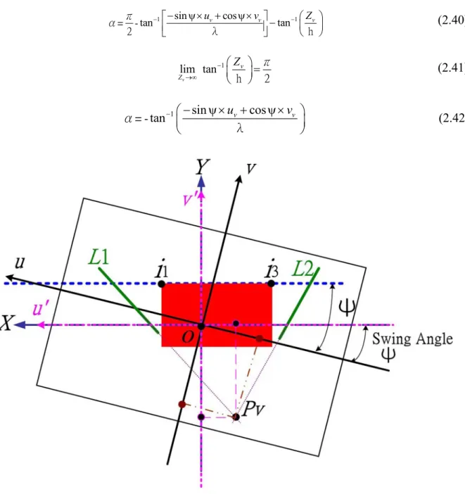
2.3.2.5 Influence of changes in camera swing angles

The swing angle, i.e. the u-v image plane rotation angle, denotes the angle between the

u-axis in the image coordinates and the X-axis in the world coordinates. As shown in Fig. 2-5,

let P1 project onto i1 and let i1 be (u, v) on the u –v plane and (u’, v’) on the u’ –v’ plane. (u, v)

and (u’, v’) are the coordinates when ψ≠0 and ψ=0, respectively. The transformation of the two coordinates can be computed by (2.37).

, , u u v v ψ ψ ψ ψ ⎡ ⎤ ⎡ ⎤ ⎡ ⎤ = ⎢ ⎥ ⎢ ⎥ ⎢ ⎥ ⎣ ⎦ ⎣ ⎦ ⎣ ⎦ cos -sin sin cos (2.37) If ψ≠0, from (1), we can obtain the results of range estimation by using (2.38).

Table 2-5 shows that the variation between the two coordinates grows with the increasing ψ,

u and v. Even if ψ is very small, it still has a great influence when the coordinates are far away

from the image center.

1 sin cos ( ) tan - tan 2 u v Z v _{= ⋅}h ⎛⎛ ⎞₋ − ⎛− ψ × + ψ × ⎞⎞ ⎜ ⎟ ⎜ ⎟ ⎜_{⎝ ⎠ ⎝ ⎠}⎟ ⎝ ⎠ π α λ (2.38)

Table 2-5 Variations between (u, v) and (u’, v’) (u’, v’)

(u, v)

ψ=1° ψ=2°

(100,200) (98.24,101.73) (96.45,103.43) (200,200) (196.48,203.46) (192.90,206.86)

Fig. 2-4 The relation between the Z-axis and the direction of movement of vehicles, denoted by Sur.