基於基因演算法應用於異質性網路單晶片系統之快速任務排程方法

(1)

國立交通大學

電子工程學系電子研究所碩士班

碩士論文

基於基因演算法應用於異質性網路單晶片

系統之快速任務排程方法

A Fast GA-Based Task Scheduling for

Heterogeneous NoC system

研究生：宓彥廷

(2)

基於基因演算法應用於異質性網路單晶

片系統之快速任務排程方法

A Fast GA-Based Task Scheduling for

Heterogeneous NoC system

研究生：宓彥廷

Student：Yan-Ting Mi

指導教授：周景揚博士

Advisor：Dr. Jing-Yang Jou

國立交通大學

電子工程學系電子研究所碩士班

碩士論文

A Thesis Submitted to

Department of Electronics and Institute of Electronics

College of Electrical Engineering and Computer Science

National Chiao Tung University

in Partial Fulfillment of the Requirements

for the Degree of Master of Science

in Electronics Engineering

August 2008

(3)

基於基因演算法應用於異質性網路單晶

片系統之快速任務排程方法

研究生 : 宓彥廷

指導教授 : 周景揚博士

國立交通大學

電子工程學系電子研究所碩士班

摘要

網路單晶片是為了應付未來極為複雜的系統單晶片的通訊需求所提出的一種新的設計方式。在這篇論文中，我們提出一個基於基因演算法的任務排程方法，把應用排程至一個異質性網路單晶片。這個任務排程方法試著去為每一個任務找到最適合的處理器，使得系統的資料處理率提升至最大。在基因演算法中，隨著任務數目的增加，排程所需的時間也會跟著增加，而且在資料處理率的表現也會變差。所以我們提出分割的基因演算法來改良這樣的狀況。實驗結果顯示，我們提出的演算法可以有效提升基因演算法的效能，而且排程時間上也有明顯的改良。

(4)

A Fast GA-Based Task Scheduling for

Heterogeneous NoC system

Student : Yan-Ting Mi Advisor : Dr. Jing-Yang Jou

Department of Electronics Engineering

Institute of Electronics

National Chiao Tung University

ABSTRACT

Network-on-Chip is a new design paradigm to meet the communication requirement of future billion-transistor System-on-Chip. In this thesis, we propose a genetic algorithm based task scheduling technique to schedule the applications to the heterogeneous Network-on-Chip architecture. The task scheduling process attempts to arrange the allocation of processor for each task such that the system throughput is maximized. In genetic algorithm, with the increasing of task number, the scheduling time will increase, and the performance in system throughput will become worse. So we propose a partition genetic algorithm to

(5)

improve this kind of situation. The experimental results show that proposed algorithm not only upgrade the performance of genetic algorithm, but also shorten the scheduling time obviously.

(6)

Acknowledgements

First of all, I would like to express my sincere appreciation to my advisor Professor Jing-Yang Jou for his guidance and instruction during my master studying. Then, I would also like to give my gratitude to my co-guidance advisor Professor Lan-Da Van for his guidance. I have the honor of being their student very much. Also, I would be indebted to Cheng-Yeh Wang, Geeng-Wei Lee, Zwei-Mei Lee, Bu-Ching Lin, and Liang-Yu Lin for their great help on my research and getting so much knowledge from them. Specially thanks to all members of EDA lab for their friendship. Finally, I would show my gratitude to my family and all my friends for their encouragement.

(7)

List of Tables

Table 4.1：The parameters of GAs ...45 Table 4.2：2-step method (Task 300/Ratio 2)...47 Table 4.3：Partition (Task 200/Ratio 2)...49 Table 4.4：Comparison under different throughput demand (Task 200/Ratio 1) ...50 Table 4.5：Comparison under different throughput demand (Task 300/Ratio 1) ...51 Table 4.6：Comparison under different throughput demand (Task 400/Ratio 1) ...52

(10)

List of Figures

Figure 1.1：NoC with 16 resources ...4

Figure 2.1：Layered-micronetwork design methodology...7

Figure 2.2：Graphic-based chromosome representation ...9

Figure 2.3：Sub-graph crossover operation ...10

Figure 2.4：Rotation and reflection of SB for the shape crossover operation ... 11

Figure 2.5：Design flow ...13

Figure 2.6：NoC platform ...14

Figure 2.7：Switch architecture ...14

Figure 2.8：Switch interface...15

Figure 2.9：Processing element model ...17

Figure 2.10：Task graph of H.263 decoder ...18

Figure 2.11：Resource requirement of tasks...18

Figure 3.1：Example of task graph...23

Figure 3.2：GA-based task-scheduling flow ...27

Figure 3.3：Example of task graph ...29

Figure 3.4：Pseudo code of the initial population process...29

Figure 3.5：Detailed demonstration of an initial solution ...30

Figure 3.6：Roulette wheel method ...31

Figure 3.7：Proposed crossover flow ...33

Figure 3.8：Partition with Blevel ...35

Figure 3.9：Adjust boundary ...37

Figure 3.10：Conditional crossover...38

Figure 3.11：Resource location ...39

Figure 3.12：Mutation operation...40

Figure 3.13：Buffer length assignment...41

(11)

Figure 4.1：Experimental flow...44

Figure 4.2：TGFF output file ...45

Figure 4.3：Improvement of 2-step method (Task 300/Ratio 2) ...48

Figure 4.4：Partition (Task 200/Ratio 2)...49

Figure 4.5：Throughput curves in 200 tasks (Ratio 1) ...51

Figure 4.8：Improvement of 4 crossover schemes (Task 200/Ratio 1) ...54

Figure 4.11：Improvement of 4 crossover schemes (Task 200/Ratio 4)...55

(12)

Chapter 1 Introduction

1.1 Technology Trend

With the advance of semiconductor technology, it is possible to integrate multi-billion of transistors on a chip. As a result, hundreds of cores (processor, DSP, FPGA, and so on) will be integrated on a single chip. However, this will introduce several new problems for designers.

First, the ever-shrinking feature size causes the gate delay scaling down linearly, while the wire delay remains constant. Thus, the wire delay will become more critical than the gate delay [1]. Although the wire delay can be managed with wire pipelining techniques, it is unavoidable for designers to deal with the problem of timing

(13)

uncertainty. On the other hand, the clock skew can not be neglected and clock synchronization becomes another problem. It is almost impossible to synchronize all components on a chip with single clock. The globally-asynchronous, locally synchronous (GALS) technique may be the most suitable solution [2].

Second, the most popular architecture in current System-on-Chip (SoC) design is shared-bus based network architecture. Nevertheless, due to the weakness of high data transmission contentions between masters, the system performance will be reduced and the power consumptions will be raised. Moreover, buses can only handle 3 to 10 computation elements [3][4][5]. Following the technology trend, communication between components becomes the bottleneck of system performance. Thus, designers should search for new communication architecture to improve this kind of situation.

Third, it becomes more complex to design a system with lots of computing components while considering the limited time to market. The traditional design flow is not sufficient to conquer this problem. The design trend is toward system level design, and a communication-driven system design methodology should be considered.

1.2 Concept of Network-on-Chip

A new design methodology called Network-on-Chip (NoC) has been presented to improve the on-chip communication, this uses the technique of computer network

(14)

and parallel computing [6]. Network-on-Chip is the concept of viewing the system as a network of cores. In many cases, on-chip network can be designed in regular structures, thus, the electrical properties of global wire can be optimized and well managed. It's helpful for using aggressive signaling circuits and reducing power dissipation [3][7]. As well, the cores can communicate with each other through the network. Obviously, the methodology of NoC not only achieves the concept of Global Asynchronous Locally Synchronous (GALS) paradigm with ease but also alleviates the wire delay problem and other DSM problems. The NoC concept enables designers to design and reuse each core designed in one synchronous clock domain, and the communications between cores through the network. Hence, components can communicate with each other asynchronously [6][8].

Compared with the traditional share-bus architecture, NoC provides better performance scalability. First, it can provide high bandwidth and reduce power consumption effectively through a Peer-to-Peer communication. Second, by managing the network channel properly, multiple communications originated by multiple cores can be handled at the same time.

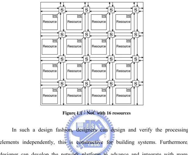
Many proposed network platforms use the regular architecture. As shown in

Figure 1.1, this is a network platform with a 2D-mesh topology. Every switch is

(15)

Figure 1.1：NoC with 16 resources

In such a design fashion, designers can design and verify the processing elements independently, this is constructive for building systems. Furthermore, designer can develop the network platform in advance and integrate with many applications [9]. Thus, we can not only amortize the development cost of network platform across many applications but also reduce time to market pressure by reuse the NoC platform.

1.3 Motivation

With the advance of the technology, while applications become more complex, the multi-core or NoC hardware will be required. When hardware design goes to multi-cores or NoC, the task scheduling becomes a important issue. Since it evolves the resources allocation and task assignment, and this is very important for system

(16)

performance and hardware utilization.

An application can be modeled as a task graph with communication and computation information. We use a heterogeneous system which includes different kind of resources for different tasks. Given a network platform with heterogeneous computing resources, the task scheduling problem is defined to decide proper allocation of resource to the task, which can in turn optimize the system performance. On the other hand, when task graph becomes more complex and task number becomes larger, traditional crossover methods can not handle the big task graphs well. Thus, we present the partition genetic algorithm method to reduce scheduling time and get better performance. It divides the task graph into several partitions by considering the execution order and communication amount between tasks.

1.4 Thesis Organization

The rest in this thesis is organized as follows. Chapter 2 introduces related works, our design flow and some basic concepts. Chapter 3 presents our task scheduling method. We use genetic algorithm with shape crossover method to reduce communication overhead, furthermore, we use partition method to improve the crossover procedure, which can lead to better throughput between generations. The experimental flow and results are shown and discussed in Chapter 4. Finally, conclusions and future works are given in the last chapter.

(17)

Chapter 2 Preliminary

In this chapter, we first introduce several related works in design methodology and scheduling. Then we talk about our design flow and NoC platform. The architecture and characteristics of our NoC platform is presented here. Finally, we introduce the concept of genetic algorithm and why it is suitable to deal with task scheduling problem.

(18)

2.1 Related Works

2.1.1 Design Methodology

There are many researches in NoC domain. In [6], it proposes using layered-micronetwork design methodology to address future SoC designs. As shown in Figure 2.1, every layer is specialized and optimized for target application domain in this vertical design flow.

Figure 2.1：Layered-micronetwork design methodology

In [10], a circuited switched two-dimensional mesh network called SoCBUS is proposed. It introduces the concept of packet connected circuit (PCC). By this theory, packet is switched through the network and locking the circuit as it goes. PCC is similar to circuit switching which has the advantage of bandwidth guarantee and deadlock-free. The integrated modeling, simulation and implementation environment are proposed In [11]. NoC infrastructure and processors are modeled, and simulation is performed to find the optimal network configuration.

(19)

[12] presents the Xpipes which contains a library of soft macros (switches, network interfaces and links), therefore, domain-specific heterogeneous architectures can be instantiated and synthesized. Xpipes provides a tool called XpipeCompiler, which can automatically instantiates a customized NoC from the library. Precisely, designer uses the library from Xpipes to describe the network architecture, and the information on the network architecture is specified in an input file for XpipeComplier. This tool can generate a SystemC hierarchical description of whole system, and it can be compiled and simulated at the cycle-accurate and signal-accurate level. [13] presents an algorithm called NMAP. It can map cores onto NOC architecture under bandwidth constraints. This can be used for both single-path routing and spilt-traffic routing. In [14], the author uses a simple packet switching communication model to reduce communication time. He proposes a two-step genetic algorithm to map a parameterized task graph onto 2D-mesh NoC architecture, which minimizes the overall execution time of the task graph.

2.1.2 Scheduling

In [15], we get the basic algorithm and concept about using genetic algorithm to deal with multiprocessor scheduling problem. We learn the partition skill to handle genetic algorithm in [16]. It provides the method to divide task graph into several partitions according to the execution time relation. Then it analyzes the benefit of partition genetic algorithm and show the experimental result to prove it. In [17] we can get the graphic based crossover method and chromosome representation thought.

(20)

It considers the communication overhead and data dependency among crossover. Since NoC is a communication-driven architecture, we consider the case when communication is the bottleneck of system. Thus, crossover with lower communication overhead can get great improvement in system performance.

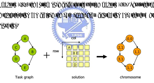
In [17] it proposes new crossover schemes which take the dependency of tasks into consideration to obtain better performance. As shown in Figure 2.2, it uses a graphical chromosome which contains the information of task graph and the allocations of tasks. For example, the top node of the chromosome indicates that task A maps to (0,0), the bottom node indicates that task E maps to (1,1). Thus, this kind of representation can include the data dependency information and this is a great innovation. A B E C D col row A C D B E 0,0 2,1 3,1 1,1 1,1 solution

Task graph chromosome A B E C D A B E C D col row A C D B E 0,0 2,1 3,1 1,1 1,1 solution

Task graph chromosome Figure 2.2：Graphic-based chromosome representation

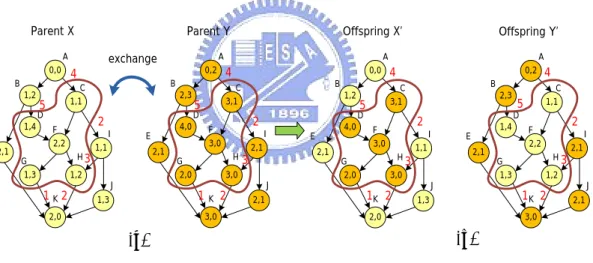
The first proposed crossover scheme in [17] is the sub-graph crossover operator which exchanges a sub-graph in a well-coded graph-based representation. The exchange process of the sub-graph crossover is illustrated in Figure 2.3. First of all, it randomly chooses a task on the task graph. For example, in Figure 2.3(a), the task F

(21)

which locates at (2,2) is chosen for Parent X and the task F which locates at (3,0) is chosen for Parent Y. Next, it selects a number x ranges from 1 to n-1 randomly, where n is the total task number of the graph. In this case, the Parent X, as shown in Figure

2.3(a), has the number x of 5. Finally, a breadth first search (BFS) is performed on

chosen task until the number of visiting tasks reaches x. As a result, it can obtain the sub-graphs in Figure 2.3(a), and it labels the communication amount for the cutting edges. For instance, the communication amount between the Task A and the Task C is 4. Finally, we exchange sub-graphs to generate the offspring X’ and Y’, the result is shown in Figure 2.3(b). 0,0 1,2 _1,1 1,4 2,2 1,3 1,2 1,1 2,1 2,0 1,3 A C B D E F I G H J K 0,2 2,3 _3,1 4,0 3,0 2,0 3,0 2,1 2,1 3,0 2,1 A C B E I G H exchange Parent X Parent Y D F J K 0,0 1,2 3,1 4,0 3,0 2,0 3,0 1,1 2,1 2,0 1,3 A C B E I G H D F J K 0,2 2,3 1,1 1,4 2,2 1,3 1,2 2,1 2,1 3,0 2,1 A C B E I G H D F J K

Offspring X’ Offspring Y’

(a) (b) 4 4 4 4 5 5 5 5 2 2 2 2 2 2 2 2 3 3 3 3 1 1 1 1

Figure 2.3：Sub-graph crossover operation

Although sub-graph crossover considers about the dependency of tasks, it is still not good enough. It can be further improved by taking the suitability between the parents and the exchanged sub-graph into account. Therefore, the author presents another crossover method by considering the communication overhead between sub-graph and surrounding tasks.

(22)

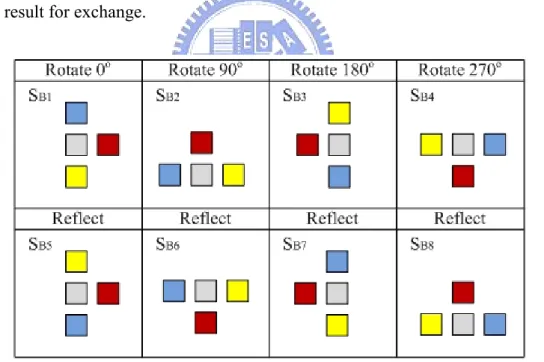
Second, in order to ease the communication cost, it proposes systematic rotation and reflection scheme to adjust one shape diagram to increase search space. For simple demonstration, in this case, it can rotate and reflect SB to obtain eight candidates as shown in Figure 2.4 named as SB1, SB2, SB3, and so on, where SB is identical to SB1. These candidates are evaluated by calculating the communication cost that they cause. The communication cost is defined as Σci*di, where ci is the

input or output communication amount of the sub-graph and di is Manhattan distance

of that communication. After calculating the communication cost for the eight candidates, it selects the candidate with the minimum communication cost as the final shape result for exchange.

(23)

2.2 Our Design Flow

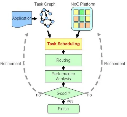
Our design flow is shown in Figure 2.5. There are two input information in our methodology. First, an application can be partitioned into communicating tasks, and the characteristics of tasks and data dependency is modeled as a task graph. Second, the NoC platform contains network architecture and heterogeneous computing resources (the task graph and NoC platform will be later explicitly explained). The task scheduling process determines which task should map to which resource. The process not only tries to reduce the communication time by mapping the interacting tasks into the same resource (make it an intra-resource communication) under memory constraints, but also tries to map tasks onto most appropriate resources to improve the computation time of each task. Next, the routing process [18] assigns a specific connect path for each communication between tasks. After the routing process, we can make a system performance analysis. If the results do not meet our requirement, we will iteratively refine our application or NoC platform and execute task scheduling and routing until the results satisfy our requirement.

(24)

Figure 2.5：Design flow

2.3 Our NoC Platform

As Figure 2.6, our NoC platform consists of switches and processing elements, each switch connects to neighbor switches and a corresponding processing element, and all of these components construct the network architecture. Processing elements can communicate with each other by passing messages through the switches of the network.

(25)

switch switch switch

PE PE PE

PE PE

PE

PE PE PE

switch switch switch

PE PE PE

PE PE

PE

PE PE PE

Figure 2.6：NoC platform

The architecture of our switch is shown in Figure 2.7. The switch has four ports connecting to neighboring switches and one port connecting to local processing element. Each port is composed of input and output stage.

(26)

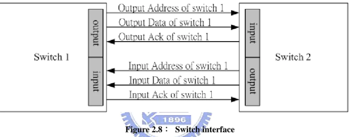
As shown in Figure 2.8, the interface of switch is composed of input and output channel. Each channel includes Address-line, Data-line and Ack-line. The Address-line delivers the input or output address of the packet. The Data-line delivers data transmitted. And the Ack-line feeds acknowledgement back to source switch or processing elements to report the result of transmission. Output channel and input channel are complementary to each other.

Figure 2.8： Switch interface

Our platform has five features: (1) circuit switching

(2) dedicated connection path (3) virtual channel flow control (4) weighted round-robin scheduling (5) pipeline bus

Feature (1) and (2) provide the bandwidth guarantee and small memory usage of network switches. Feature (3) and (4) can prevent deadlock and improve the utilization of network. Finally, feature (5) can improve the performance of network.

(27)

The details of switch and network architecture are explicitly described in [18]. There are two kinds of processing element in our NoC platform, processor and FPGA. This makes the NoC platform a fully programmable platform. It undoubted that processor is a programmable processing element. FPGA is a dedicated hardware that can be reconfigured when designing. Since our platform is fully programmable, we can reduce the development cost by reuse it in many different applications without any architectural modification.

The processor is highly flexible processing element. It can execute tasks with nice management. But in most cases, processors cannot provide better performance than a dedicated hardware in executing tasks with data dependency. On the other hand, dedicated hardware cannot have good flexibility like processors. Hence, our platform contains another type of processing element to overcome this issue. An FPGA work like a dedicated hardware, but it has the advantage of being reconfigured in design period. Consequently, our platform has the ability to execute various tasks efficiently.

Figure 2.9 shows both the processor and FPGA model. Every processing element

contains a network interface(NI) to communicate with local switch. The buffer is temporary memory which uses for storing the input and output data when communicating with other processing elements. As before-mentioned, our platform is consisting of two different types of processing elements. FPGA contains a FPGA core, and processor contains a processor core and local memory, which can store the program and intermediate data in execution.

(28)

buffer NI FPGA buffer NI FPGA buffer NI Processor memory buffer NI Processor memory

Figure 2.9：Processing element model

2.3.1 Task Graph

Applications can partition into many tasks due to the parallelism. Figure 2.10 shows a task graph example which is a H.263 decoder. A node represents a task and it functionality. Take node C as an example, it functionality is IDCT which performs an inverse discrete cosine transformation of a frame produced by task B. The edge represents a data transmission and it communication amount. For instance, when task B has completed, it transmit c2 unit data to task C. An edge also shows the data dependency between tasks, a task cannot be executed until it receives the data from all its predecessor. For example, task G cannot be executed until it receives c5 unit data from task D and c6 unit data from task E, this can insure the correctness of program.

(29)

B IQ C IDCT E R P-f D R I-f c1 A VLD G out c2 c4 c3 c5 c6 B IQ C IDCT E R P-f D R I-f c1 A VLD G out c2 c4 c3 c5 c6

Figure 2.10：Task graph of H.263 decoder

In addition to the task graph, there is a processing element database to specify the details of tasks when performing on the specific processing elements. As shown in Figure 2.11, processing element database contains the executing time of the task and the memory usage (program and intermediate data) when executing on a processor. If the task is executing on an FPGA, it shows the execution time and the capacity usage (logics) of the task.

FPGA Processor task ∞ , ∞ 6 , 8 6 , 8 10 , 10 3 , 4 4 , 6 (e, c) 10 , 10 12 , 10 12 , 10 15 , 12 5 , 8 10 , 4 (e, m) VLD IDCT out R P-f R I-f IQ e : executing time m : memory usage c : capacity usage ∞ , ∞ 6 , 8 6 , 8 10 , 10 3 , 4 4 , 6 (e, c) 10 , 10 12 , 10 12 , 10 15 , 12 5 , 8 10 , 4 (e, m) VLD IDCT out R P-f R I-f IQ FPGA Processor task e : executing time m : memory usage c : capacity usage

(30)

2.3.2 Performance Evaluation

Since the application is executed consecutively, we take throughput instead of execution time as the system performance metric. Take video compressing as an example, we may compress the entire movie into a more compact form, like Mpeg4. A movie may contain thousands of frames, therefore, when we evaluate the system performance of the video compressing ability, we may take frame per second as the rating of system performance rather than second per frame. As a result, we take throughput as the metric of system performance. More precisely, our system performance evaluation is to calculate how many times the application can be performed in a period.

2.4 Genetic Algorithms

Task scheduling tries to allocate a set of tasks to resources such that the performance is optimal. Nevertheless, it is known as NP-complete. Therefore, people often use heuristic algorithms to deal with task scheduling problem [14][18][19][20][21].

In considering about the system performance, there are several important aspects. First, since the NoC platform contains heterogeneous computing resources, and tasks maybe suited to be executed on some kind of resources, thus, the execution time of a task depends on the resource it used. Second, the communication time

(31)

between tasks highly depends on the communication distance. Therefore, communication time can be greatly improved by mapping the communicating tasks onto the same resources. However, this may violate the constraints as mention before. Moreover, the suitability of tasks and resources are neglected. As the result, the task scheduling problem must be solved with considering the trade-off among execution time, communication time and constraints.

Typically, Genetic algorithms are good at finding near-optimal solutions in a large search-space. As well, genetic algorithms do not require the knowledge of the search-space, they only need a measure of solution, it differ from many traditional optimization techniques [14][22][23]. In other words, we do not need to know how to arrange these tasks to get the best performance, we only have to define the performance of the solution. As a result, Genetic algorithms are quite suitable for the task scheduling problems.

Genetic algorithms are search algorithms based on the mechanics of natural selection and natural genetics. Genetic algorithms are different from other traditional optimization methods in very four fundamental ways [22] :

(1) Genetic algorithms use a coding of the parameter set instead of parameters themselves.

(2) Genetic algorithms search from a population of search nodes rather than a single one.

(32)

auxiliary knowledge.

(4) Genetic algorithms use probabilistic transition rules, not deterministic rules.

In order to employ genetic algorithms to solve our problem, first we need to encode the possible solutions of the optimization problems as a set of chromosomes. Each chromosome represents a solution to the problem, and a cluster of solutions form a population. Next we generate the initial population, the chromosomes in the initial population are often generated randomly or heuristically. After that, we have to evaluate the fitness value of the chromosomes, this can judge how good the chromosome is to the problem, and it is important in the procedure of evolution.

In evolution process, we optimize the population by using genetic operators: selection, crossover and mutation. The genetic algorithms select chromosomes from current generation by their fitness value. The higher fitness value the chromosome has, the higher probability it will be selected. In crossover and mutation procedures, next generation is generated by means of exploring the search-space. Finally, we evaluate the fitness value of chromosomes in the next generation, then add them into the current generation. In order to keep the size of population, some bad chromosome will be discarded. We can pick the better result generation by generation until the saturation condition is met, and we can find the solution in the best chromosome when genetic algorithms terminate.

(33)

Chapter 3 Task Scheduling

In this chapter, the proposed task scheduling method is presented. Procedures of our method will be explained explicitly in following articles. In addition, we will discuss the partition work and communication improvement in our algorithm into depth. We believe that proposed algorithm can improve the scheduling result and shorten scheduling time obviously.

(34)

3.1 Assumption

First, we need to define the constraints and make some assumptions.

There are two ways to implement a task, software(program) or hardware (logic). Since local memory of processor and total capacity of the FPGA is limited, we should consider these two constraints. Memory constraint of processor restricts the size of programs and intermediate data of tasks. The capacity constraint of an FPGA is similar to memory constraint. It limits the total logics of tasks which are assigned to an FPGA.

There should be some buffers for performing a task. For instance, in Figure 3.1 we can see, before task A is executed, it has to wait for 4 units data from task B and 2 units data from task C. Totally, task A needs 6 units input buffer for these input data. Besides, when task A is executing, the generated result needs to be stored in output buffer. Therefore, the minimum buffer requirement is 9 units.

D C B A 4 2 3 D C B A 4 2 3

(35)

However, this is not sufficient if our buffer has only the summation of input data and output data. First, when task A is executing, it receives 4 units data from task B and 2 units data form task C and stores them in input buffer. Moreover, the output buffer should prepare 3 units data for result of task A, and these requirements fill the buffer. Thus, neither task B nor task C can transmit data to task A until this job is finished, and this prevent the system from being executed continuously. Second, if output buffer of task A is full (task D does not finish receiving data from task A), it has to wait until the output buffer is clear, which means that it is idling during this period. Hence, in order to overcome this problem, we set our minimum buffer requirement to 18 units, which is twice of the minimum buffer requirement. Then the task can receive and transmit data whenever task is executed or not. This can greatly improve the system performance.

We don’t need to decide the execution order when more than two tasks are allocated to the same FPGA, because tasks are implemented in different parts of FPGA, none of them use the same component of the FPGA. But when more than two tasks are allocated to the same processor, the situation is different, we have to decide the execution order dynamically. It is not fitting to decide the execution order of the tasks in advance because of the dynamic behavior of communication. In addition, before the task is executed, it has to wait for all its input data.

(36)

According to above reasons, we choose a dynamic First In First Serve(FIFS) strategy to determine the execution order of tasks. It has two advantages. (1)Flexibility to conquer the uncertainty of network. (2)Raise the utilization of processor by considering about the data availability of tasks [24]. A FIFS strategy is implemented as a queue. The task is pushed into the queue when all the input data are ready and output buffer size is sufficient. Then processor can execute the tasks according to the order.

3.2 Problem Formulation

Task scheduling problem can be formulated as follows: Given:

(1) A task graph G(V,E) with communication and computation information (2) An NoC platform with following characteristics:

(a) mesh size

(b) memory size of processor (c) capacity size of FPGA

(d) buffer size of processing element

(37)

Goal:

Use our algorithm to efficiently schedule each task to maximize system throughput

3.3 GA-based Task Scheduling Flow

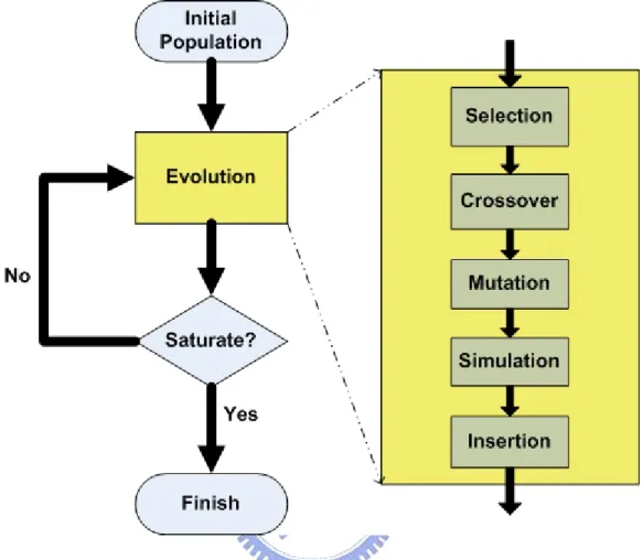
The proposed GA-based task scheduling flow is illustrated in Figure 3.2. It includes the following procedures. Initial population and evolution composed of selection, crossover, mutation, simulation and insertion. First, we generate the initial population. Then the evolution process tries to explore the search space until it reaches the saturation condition we set. Finally, the best chromosome in the population is our solution.

(38)

Figure 3.2：GA-based task-scheduling flow

3.4 Initial Population

We use a meta-random scheme to generate the initial population of chromosome and it is divided into two steps:

(1) We use topological sorting scheme to sort the tasks in the task graph. (2) The tasks are mapped onto the NoC platform in this order.

(39)

In step 2, we must consider 3 conditions:

(a) If the task has no precedence, the task is mapped randomly.

(b) If the task has only one precedence, the task is mapped according to the allocation of its precedence.

(c) If the task has more than one precedence, the task is mapped according to the allocation of its precedence and the communication amount between the task and its precedence.

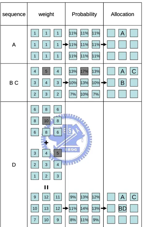
We take Figure 3.3 as an example to demonstrate initial population, and the mapping steps of initial population are illustrated in Figure 3.5. First, a topological sort is performed on the task graph, and the topological order is given by A, B, C, and D. Next, task A is randomly mapped to the NoC platform. Then, task B and task C are mapped according to the allocation of task A. Comparing to task D, task B and task C have a higher probability of being mapped onto the allocations close to task A. Finally, task D is mapped according to the allocations of task B and task C. As we can see, edge B→D and edge C→D have different communication amounts. Thus, the probability should be higher for the allocations that are nearer to task B than those nearer to task C. By above descriptions, we can summarize the initial population process as listed in Figure 3.4, where the ticket in the pseudo code [22] means the probability.

(40)

D C B A 2 1 2 3 D C B A 2 1 2 3

Figure 3.3：Example of task graph

1. topological sort

2. according to the topological sort order, place the tasks. 2.1 random place the root since it has no parent 2.2 foreach task T in topological sort order

{ find free allocations (free resources) for T for each free allocation X

{ //calculate the ticket of X ticket = 0

for each parent P of the task

{ //the nearer of the distance between //the tasks, the higher of the ticket points //the more of the communication amount, //the higher of the ticket points

ticket += [(row_max+col_max-1)-manh_distance(X, P)] * Commu_amount(T,P) }

}

place the task T according to the location of its parent(s) using roulette wheel method [32]

}

[22]

(41)

A 11% 11% 11% 11% 11% 11% 11% 11% 11% 13% 17% 10% 7% 10% 13% 13% 10% 7% A

sequence Probability Allocation

A B C B C 6 8 8 6 8 10 6 8 6 3 4 2 1 2 3 5 4 3 9 12 10 7 10 13 11 12 9 9% 13% 11% 8% 11% 14% 12% 13% 9% A BD C D 1 1 1 1 1 1 1 1 1 4 5 3 2 3 4 4 3 2 weight A 11% 11% 11% 11% 11% 11% 11% 11% 11% 13% 17% 10% 7% 10% 13% 13% 10% 7% A

sequence Probability Allocation

A B C B C 6 8 8 6 8 10 6 8 6 3 4 2 1 2 3 5 4 3 9 12 10 7 10 13 11 12 9 9% 13% 11% 8% 11% 14% 12% 13% 9% A BD C D 1 1 1 1 1 1 1 1 1 4 5 3 2 3 4 4 3 2 weight

(42)

There are two reasons for us to use a meta-random scheme to generate chromosomes. First, a pure random scheme may cause a very poor performance. Second, the diversity of the chromosomes in the initial population should be kept as high as possible, this can in turn the genetic algorithms to have a higher probability of exploring a larger search-space. As a result, a meta-random scheme is used to generate the chromosomes.

3.5 Selection

Because of the principle of eugenics, an individual chromosome with a higher fitness value has a higher probability to produce another generation. Hence, pairs of parents from the population were selected using the roulette wheel method. Each chromosome in the population has a roulette wheel slot which is proportional to its fitness value. Then we can select the chromosome by spinning the roulette wheel. As illustrate in Figure 3.6, Chromosome A has the largest fitness value, so it occupies the largest space in the roulette wheel. The selected chromosomes will mate in the next stage by spinning the roulette wheel many times.

A chromosome B C D E 5 fitness 4 2 3 1 A B C D E spin A chromosome B C D E 5 fitness 4 2 3 1 A B C D E spin A B C D E spin

(43)

3.6 Crossover

3.6.1 Proposed Crossover Method

The genetic algorithms use crossover to find the local optimal point. In nature, offspring inherit their features from their parents. For instance, if parents are tall, they often have tall children. So as in the genetic algorithms, the generated chromosomes inherit their features from their parents. Nowadays, we have many new applications with high complexity, follow the trend, the task graph will become more complex, and task number will become larger. In this situation, scheduling time will become longer, and we need more time to find a better solution for system performance. Hence, this is a good issue for us to research.

If we examine traditional crossover algorithms carefully, we can find that these algorithms just randomly select a part of chromosome to exchange. When task graph becomes larger, some parts of tasks in the graph are always being neglected for crossover selection. However, they may have great opportunities for throughput improvement. That is, such crossover algorithm can not handle a large task graph well. This situation will become worse when task number become larger. As a result, we must use some new crossover algorithm to overcome this weakness.

Our modified crossover flow is shown in Figure 3.7. First, we divide the task graph into several partitions by the execution order in the system, and then adjust the boundary according to the communication amount. Next, we select sub-graphs in

(44)

every partition and find the best shape which has the minimum communication overhead with surroundings [17]. In order to further control the communication overhead, we use a value to filter the crossover in every partition. If the communication overhead is larger than this value, we will not do the crossover. After that, we go to next partition and repeat the procedure.

(45)

3.6.2 Partition

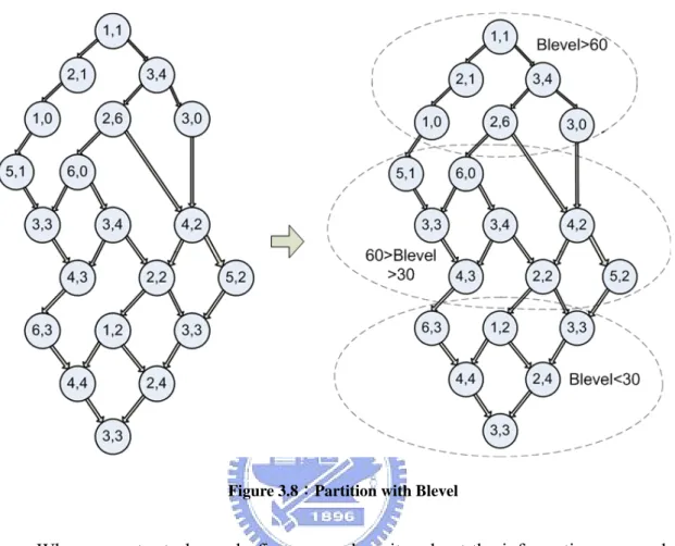
In [16], it presents a partition genetic algorithm. We use the partition method in this article to divide the task graph into several partitions, and do the crossover in each partition. This article introduces the concept of blevel, which represents the execution order of the system. Partition method can make the crossover more balance in the task graph and get better result of scheduling. However, this crossover method doesn’t consider about the data dependency. It just uses the traditional chromosome to do crossover, and this will cause a bad simulation result. Therefore, we use the graphic-based chromosome [17] to solve this problem and do some further improvement to get our own crossover algorithm.

As shown in Figure 3.8, we use the value of blevel to divide the original chromosome into three partitions. Since the task number becomes smaller, crossover method can run more balance in the partitions.

(46)

Figure 3.8：Partition with Blevel

When we get a task graph, first we analyze it and get the information we need. Next, we have to decide how many partitions are suitable for the original task graph. Number of partitions influences the result of crossover. If the partition number is too small, then we won’t get great improvement in scheduling result. On the other hand, if the number of partitions is too big, then there will be heavy communication overhead and bring in worse result. Moreover, the partition number is related to scheduling time of each generation. Too many partitions will bring in longer scheduling time. Thus, the number of partitions is very important. In our algorithm, we divide the task graph by 30 tasks a partition. For example, if we have 200 tasks, then we will have 7 partitions in this task graph. We think this is a suitable partition

(47)

size for our algorithm since it can run our crossover method well and handle the communication overhead.

After deciding the partition, we adjust the partition boundary for task graph. Since we want to reduce the communication between different partitions, we adjust the boundary to make the communication amount between different partitions become lower. When we do the crossover, we only pick tasks which are in the same partition. However, this crossover damages the allocation in initial population and cause heavy communication overhead between different partitions. As a result, if we can control the communication overhead between different partitions, this will improve the crossover result.

As a result, our strategy is shown in Figure 3.9. Task A has 4 units communication with next partition and 5 units inner communication, so we keep task A in the origin partition. Task B has 5 units communication with next partition and 6 units inner communication, so we keep it, too. Finally, Task C has 10 units communication with next partition and 7 units inner communication, therefore, we move it to the next partition. This procedure can reduce the communication between different partitions from 10 to 7.

(48)

Figure 3.9：Adjust boundary

3.6.3 Conditional Crossover

NoC architecture is communication-driven system. If we can do some improvement by considering communication overhead in each crossover, then we can get great improvement in the throughput of every generation. Thus, we can calculate the communication overhead of each crossover, and determine a value to judge whether to do the crossover or not. As Figure 3.10, we calculate the communication overhead of three sub-graphs as 35,25 and 32, and we use value 30 to filter each crossover, so we do the second crossover and cancel others.

This value can decide by experience and the parameters of the system. To sum up, our strategy is we choose a sub-graph and find the best shape, than we calculate

(49)

the communication overhead to decide if we do the crossover or not. Because of the partition, we do more than one crossover in each generation, so we can use this value to filter crossover and get better result.

Figure 3.10：Conditional crossover

3.6.4 Task Range

We use the partition technique to handle task graphs with different task sizes. We choose three sizes in our experiments, they are 200, 300 and 400 tasks in each task graph. We think that mesh size of NoC architecture influences the system performance. Every task range has a suitable mesh size, if we use a small mesh size to run a big task graph, then the system bottleneck may fall on the NoC architecture. However, our focus is on the task scheduling algorithm, so we choose these 3 task

(50)

sizes and use the same mesh size 7*7(as Figure 3.11) for NoC architecture. If the complexity of a system is closer to the limitation an NoC architecture can provide, our scheduling algorithm can only achieve little improvement on the system throughput.

Processor

FPGA Processor

FPGA

Figure 3.11：Resource location

3.6.5 Two-Step Crossover

In the procedure of genetic algorithm, partition algorithm can get great improvement at the start of evolution. However, when chromosome is improved to certain degree, it becomes harder to get a better result by every crossover. In order to overcome this problem, we have to find a suitable crossover strategy in the later generation. Every crossover method has it own throughput curve and characteristic. If we can use other crossover method in the later generation to get better improvement through the whole evolution procedure of genetic algorithm, that will be a great solution to the scheduling problem.

(51)

In our algorithm, we change the crossover frequency from once in every partition to once in whole task graph. The consideration is like Simulated Annealing algorithm, when chromosome improves to certain degree, we change the crossover strategy to gradually approach better performance. Hence, we switch the crossover method at the 200th_{generation, since it is the threshold point of improvement in our} algorithm. After that, the improvement of our algorithm becomes worse. As a result, we use a two-step crossover method to get better improvement through the evolution procedure.

3.7 Mutation

We use the operator mutation to prevent the genetic algorithms from just finding a local optimal point. It may have the opportunity to reach or approach the global optimal by randomly changing the feature of the chromosome. The proposed mutation scheme is shown in Figure 3.12. It first selects a task randomly, then the

selected task has a probability to move to a random allocation. This probability is decided by user according to their experience.

D C E B

A

1. Randomly select a task : task E D C B E A 2. Randomly move to new allocation D C E B A

1. Randomly select a task : task E D C B E A 2. Randomly move to new allocation

(52)

3.8 Simulation and Insertion

After crossover and mutating, it is necessary to evaluate the fitness value of each newly generated chromosome. Due to the dynamic situation (e.g. the execution order of the tasks in a processor) during the consecutive execution of the application on the proposed platform, a discrete event simulation is used to obtain the throughput of every newly generated chromosome.

Before simulation, the buffer length assignment of each task is conducted. The Input and the output buffers of PEs are assigned equally to each port of task. For example, in Figure 3.13, there are two tasks assigned to PE, T1 and T3 respectively. In order to perform the discrete-event simulation with the FIFS manner, several buffers are assigned to the input and output ports of the tasks.

buffer T1 T3 Buffer NI T1 T3 buffer T1 T3 Buffer NI T1 T3

Figure 3.13：Buffer length assignment

On the other hand, the XY routing is used to route the communication paths to estimate communication effect and by assuming that contention will always occur.

(53)

After calculating the fitness value of every new chromosome, we insert these chromosomes into current population. We have to remove some chromosomes because of the fixed population size. As Figure 3.14, after inserting new chromosomes to current population, we sort the population in decreasing order with fitness value. According to selection of natures, chromosomes with low fitness value are discarded, and this can keep a fixed-size population.

Figure 3.14：Insertion

3.9 Termination

During the evolution process, our genetic algorithms will be terminated when fitness value of the best chromosome is saturated or the generation number reaches a pre-defined number.

(54)

Chapter 4 Experimental Results

In this chapter, first we introduce our experimental environment and settings. Next, we provide the comparison between our crossover algorithm and others through the experimental results. It turns out that the proposed algorithm has better performance than others.

(55)

4.1 Experimental Environment and Flow

Our experimental flow is shown in Figure 4.1. First, we use TGFF [25] to generate random cases, where TGFF is a user-controllable, general-purpose, pseudorandom task graph generator. Next, the generated task graphs are scheduled by our task scheduling program. Finally, we can analyze the experimental results.

Task Graph TGFF Task Analysis Scheduling Task Graph TGFF Task Analysis Scheduling

Figure 4.1：Experimental flow

We use TGFF to generate many task graphs for our experiments. As shown in

Figure 4.2, the bottom-left is a netlist, “TASK” represents a task and the following

statements are the task name and task type. For instance, task “t0_0” is a “TYPE 2” task, and we can find the corresponding information in the computation table in the top-right of Figure 4.2. “uP” and “fpga” represents the computation time in processor and FPGA respectively. “memory” and “capacity” are the memory and capacity usage of processor and FPGA. “ARC” represents a data transmission form the former to the later, and the communication table (top-left of Figure 4.2) indicates the corresponding communication amount.

(56)

@computation 0 {

#---# type uP memory fpga capacity

0 55.7067 163.892 151.128 178.518 1 64.9349 152.398 159.265 175.757 2 75.4444 160.801 166.259 193.153 3 52.5038 157.158 152.051 153.982 4 66.1995 175.019 170.291 192.132 5 56.5161 151.905 154.492 159.021

.

} @communication 0 { #---# type amount 0 155.707 1 151.676 2 158.991 3 153.979 4 194.139 5 160.684

.

} @TASK_GRAPH 0 { PERIOD 1659 TASK t0_0 TYPE 2 TASK t0_1 TYPE 73 TASK t0_2 TYPE 14 TASK t0_3 TYPE 51

ARC a0_0 FROM t0_0 TO t0_1 TYPE 35 ARC a0_1 FROM t0_0 TO t0_2 TYPE 11 ARC a0_2 FROM t0_1 TO t0_3 TYPE 30 ARC a0_3 FROM t0_2 TO t0_3 TYPE 47 } t0_3 51 t0_2 73 t0_1 14 t0_0 2 30 47 35 11 @computation 0 { #---# type uP memory fpga capacity

0 55.7067 163.892 151.128 178.518 1 64.9349 152.398 159.265 175.757 2 75.4444 160.801 166.259 193.153 3 52.5038 157.158 152.051 153.982 4 66.1995 175.019 170.291 192.132 5 56.5161 151.905 154.492 159.021

.

} @communication 0 { #---# type amount 0 155.707 1 151.676 2 158.991 3 153.979 4 194.139 5 160.684

.

} @TASK_GRAPH 0 { PERIOD 1659 TASK t0_0 TYPE 2 TASK t0_1 TYPE 73 TASK t0_2 TYPE 14 TASK t0_3 TYPE 51

ARC a0_0 FROM t0_0 TO t0_1 TYPE 35 ARC a0_1 FROM t0_0 TO t0_2 TYPE 11 ARC a0_2 FROM t0_1 TO t0_3 TYPE 30 ARC a0_3 FROM t0_2 TO t0_3 TYPE 47 } t0_3 51 t0_2 73 t0_1 14 t0_0 2 30 47 35 11 t0_3 51 t0_2 73 t0_1 14 t0_0 2 30 47 35 11

Figure 4.2：TGFF output file

In this experiment, we compare the traditional crossover schemes and our crossover schemes. The parameters of GAs are shown in Table 4.1.

Table 4.1：The parameters of GAs

1000 Max generation 400 Population 20% Mutation rate 40% Cross rate 1000 Max generation 400 Population 20% Mutation rate 40% Cross rate

(57)

Cross rate means that 40% of population is going to mate. Mutation rate means that every new generated chromosome has the probability of 20% to perform mutation. And the whole population is set to 400 chromosomes. Algorithm will terminate until the performance of the best chromosome is saturated or when it reach max generation.

We generate 20 random task graphs in each experiment, and we use three task ranges as 200, 300 and 400 tasks in each task graph. The computation time of each task is set to 150 ~ 200 time unit on FPGA and 50 ~ 67 time unit on processor. When there is two or more than two tasks map onto a processor, the processor needs to schedule the tasks. Therefore, we set the computation time of each task on processor 1/3 times of that on FPGA such that the computation time of each task on processor or FPGA is more balanced. The communication amount is 150 ~ 200 unit data, and the maximum fanin/out of each task is 6. The memory and capacity usage of each task is set to 150 ~ 200.

The memory of processor and capacity of FPGA are set to 1,800. The communication time is the communication amount divided by channel bandwidth without any contention. We set the channel bandwidth to 1 ~ 4 (unit data/ unit time), such that the ratio of computation time to communication time (no contention) is 1 ~ 4. When the ratio is low (e.g., 1), the system is communication intensive, when the ratio is high (e.g., 4), the system is computation intensive. We use this ratio to define the environment of below experiment.

(58)

4.2 Analysis

1. 2-step VS. 1-step

We compare three crossover schemes here. The curve “Shape” is the crossover scheme as presented in [17]. Curve “Shape + Partition” means using partition cross through the evolution process and curve “2-step” is our crossover scheme. As we can see in

Figure 4.3, if we change the crossover method in the 200th generation, we can get

better performance in the later generation. In this case, we can get 4.6% throughput improvement in 1,000th_{generation, and the throughput of 2-step method is always} better than the shape method.

Table 4.2：2-step method (Task 300/Ratio 2)

2-step Shape + Partition Shape

Generation 100 200 600 1000 100 200 600 1000 100 200 600 1000

(59)

400 450 500 550 600 650 700 100 200 600 1000 Generation Throughput 2-step Shape+Partition shape

Figure 4.3：Improvement of 2-step method (Task 300/Ratio 2)

2. Partition Method

As shown in Figure 4.4, three curves show the throughput in 100th, 200th and 1,000th_{generation. Since we use partition cross with control of communication} overhead, we can get a raising trend when partition number increases. But partition number influences the run time of system, so we pick a proper value of partition by the improvement curve. Take Figure 4.4 as an example, when partition number is more than 6, the throughput improvement curve becomes flat.

(60)

Table 4.3：Partition (Task 200/Ratio 2) Partition 1 2 3 4 5 Throughput at 100gen 621 663.1 671.8 671.4 682.6 Throughput at 200gen 679.3 740.7 749.7 746.1 749.4 Throughput at 1000gen 783.1 845 852.8 857.5 840 Partition 6 7 8 9 10 Throughput at 100gen 685 679.6 694 691.7 700.8 Throughput at 200gen 755.8 760.3 767.6 767.8 766 Throughput at 1000gen 863.9 873.4 884.2 871.6 890.3 600 650 700 750 800 850 900 1 2 3 4 5 6 7 8 9 10 Partition number Throughput 1000 gen 200 gen 100 gen

(61)

3. Comparison under Different Throughput Demand

We compare three crossover schemes under 3 task ranges including two-point crossover, shape crossover [17] and our crossover method. The advantages of our algorithm are proved here. Because of great improvement of throughput in the beginning of evolution, we can save a lot of time compared with other crossover schemes under different throughput demands. Especially in terms of tasks of 300 and 400, the saving time is significant.

Table 4.4：Comparison under different throughput demand (Task 200/Ratio 1)

Task200

Throughput 250 350 450

2 point 29 243 837

Shape 13 233 631

(62)

0 100 200 300 400 500 600 700 800 900 250 350 450 Throughput Generation 2 point Shape 2-step

Figure 4.5：Throughput curves in 200 tasks (Ratio 1)

Task300

2 point 105 364 868

Shape 88 259 672

(63)

0 100 200 300 400 500 600 700 800 900 1000 200 250 300 Throughput Generation 2 point Shape 2-step

Task400

PP 12 150 713

Shape 5 161 469

(64)

0 100 200 300 400 500 600 700 800 160 200 240 Throughput Generation 2 point Shape 2-step

4. Throughput Comparison

In this section, we compare four crossover methods including random, two-point crossover, shape crossover [17] and our method. We normalize the throughput to random method. As we can see, we can get around 10% improvements in 100th generation in all cases. If we can get great improvement in the start of evolution, then we can save a lot of time to obtain a desired throughput.

In most cases, our algorithm can attain higher throughput in the whole evolution process, especially for the case of task number above 300, where 5% improvement can be attained at 1,000th_generation.

(65)

Task200

1 1.1 1.2 1.3 1.4 1.5 1.6 1.7 1.8 1.9 2 100 200 400 600 800 900 1000 Generation Throughput 2-step Shape 2 point Random 8.2%

Figure 4.8：Improvement of 4 crossover schemes (Task 200/Ratio 1)

1 1.1 1.2 1.3 1.4 1.5 1.6 1.7 1.8 1.9 100 200 400 600 800 900 1000 Generation Throughput 2-step Shape 2 point Random 10%

(66)

1 1.1 1.2 1.3 1.4 1.5 1.6 1.7 1.8 1.9 100 200 400 600 800 900 1000 Generation Throughput 2-step Shape 2 point Random

(67)

There are 4 cases of task graphs containing 170~230 tasks under 4 ratios of computation time to communication time. Our algorithm can obtain 8%~10% improvement in 100th_{generation, but in the later generation, the difference is} decreased.

Task300

(68)

1 1.1 1.2 1.3 1.4 1.5 1.6 1.7 1.8 1.9 0 200 400 600 800 1000 1200 Generation Throughput 2-step Shape 2 point Random 12.1

(69)

There are 4 cases of task graphs containing 270~330 tasks under 4 ratios of computation time to communication time. Our algorithm can obtain 12% improvement in 100th_{generation, and we can still have above 4% improvement in} 1000th generation.

(70)

Task400

1 1.1 1.2 1.3 1.4 1.5 1.6 1.7 1.8 0 200 400 600 800 1000 1200 Generation Throughput 2-step Shape 2 point Random 13.2%

(71)

1 1.1 1.2 1.3 1.4 1.5 1.6 1.7 1.8 0 200 400 600 800 1000 1200 Generation Throughput 2-step Shape 2 point Random

There are 4 cases of task graphs containing 370~430 tasks under 4 ratios of computation time to communication time. Our algorithm can attain above 12% improvement in 100th_{generation, and we can still have above 5% improvement in} 1000th generation.

(72)

5. Mutation Rate VS. Throughput

250 260 270 280 290 300 310 320 330 340 350 0 200 400 600 800 1000 1200 0 10% 20%

Figure 4.20：Mutation rate VS. Throughput (Task 300/Ratio 2)

In our algorithm, suitable mutation rate can raise throughput performance. However, we think that crossover method dominates the throughput performance of genetic algorithm. Thus, we focus on the improvement of crossover method.

(73)

Chapter 5 Conclusions and future work

5.1 Conclusions

Our method can obtain great improvement in scheduling process. We can use the result according to our requirement. For instance, if we want to get a throughput in a short period, our method can attain around 10% improvement in 100th generation. If our requirement is met around here, we can save a lot of scheduling time. On the other hand, if we want a higher throughput, our method can also provide better throughput in the later generation. Especially for the case of task number above 300, our method can still obtain 5% improvement at the 1000th generation.

(74)

Traditional method can not handle the task graph well, and this kind of situation will become worse when task graph become larger. So we combine the partition scheme and graphic-base crossover to improve the partition method by finding suitable partition size and adjust boundary. Experimental result shows that the improvement in throughput is obvious and we can save a lot of scheduling time. When applications become more complex, we think that our scheduling method can handle well and get great system performance.

5.2 Future work

Partition method for task graph is important for partition genetic algorithms, especially in the complex applications. If we can find better partition method to handle the task graph, we believe that we can speed up the scheduling program and obtain better performance in system throughput. In order to get better partition algorithm, we can further consider about the partition size, communication amount, and task topology.

We can find different improvement curves in different crossover methods. For example, our method can obtain great improvement at the start of evolution, but in later generation, there is still space for further improvement. In other traditional method, they have their own curves and trend. If we can do some detail analysis about all the crossover methods, maybe we can find a better crossover method by combining their advantage.

(75)

Reference

[1] R. Ho, K. Mai, and M. Horowitz, "The future of wires," IEEE, vol. 89, no. 4, pp. 490-504, April 2001.

[2] William J. Dally and J. Poulton, "Digital Systems Engineering," Cambridge

University Press, 1998.

[3] Cesar Albenes Zeferino and Altamiro Amsdeu Susin, "SoCIN: A Parametric and Scalable Network-on-Chip," 16th Symposium on Integrated Circuits and

Systems Design, pp. 169-174, Sep. 2003.

[4] Axel Jantsch, and Hannu Tenhunen, "Networks on Chip," Kluwer Academic

Publishers, 2003.

[5] Adrijean Adriahantenaina, Hervé Charlery, Alain Greiner, Laurent Mortiez and Cesar Albenes Zeferin, "SPIN: a scalable, packet switched, on-chip micro-network," Design, Automation and Test in Europe Conference and

Exhibition, supplements 70-73, 2003.

[6] Luca Benini and Giovanni De Micheli, "Networks on Chips: a New SoC Paradigm," Computer, Volume 35, Issue 1, pp. 70-78, Jan. 2002.

[7] William J. Dally and Brian Towles, "Route Packets, Not Wires: On-Chip Interconnection Networks," Design Automation Conference, pp. 684-689, June 2001.

(76)

[8] Pierre Guerrier and Alain Greiner, "A Generic Architecture for On-Chip Packet-Switched Interconnections," Design, automation and test in Europe, pp. 250-256, 2000.

[9] Shashi Kumar, Axel Jantsch, Juha-Pekka Soininen, Martti Forsell, Mikaek Millberg, Johny Öberg, Kari Tiensyrjä and Ahmed Hemani, "A Network on Chip Architecture and Design Methodology," IEEE Computer Society Annual

Symposium on VLSI, pp. 105-112, April 2002.

[10] Daniel Wiklund and Dake Liu, "SoCBUS: Switched Network on Chip for Hard Real Time Embedded Systems," Parallel and Distributed Processing

Symposium, April 2003.

[11] Doris Ching, Patrick Schaumont and Ingrid Verbauwhede, "Integrated modeling and Generation of a Reconfigurable Network-on-chip," 18th International

Parallel and Distributed Processing Symposium, pp. 139-145, 2004.

[12] Davide Berozzi and Luca Benini, "Xpipes: A Network-on-Chip Architecture for Gigascale Systems-on-Chip," Circuit and Systems Magazine, Volume 4, Issue 2, pp. 18-31, 2004.

[13] Srinivasan Murali and Giovanni De Micheli, "Bandwidth-Constrained Mapping of Cores onto NOC Architectures," Design, Automation and Test in Europe

基於基因演算法應用於異質性網路單晶片系統之快速任務排程方法

國 立 交 通 大 學

電子工程學系 電子研究所碩士班

碩 士 論 文

基於基因演算法應用於異質性網路單晶片

系統之快速任務排程方法

A Fast GA-Based Task Scheduling for

Heterogeneous NoC system

研 究 生 ： 宓 彥 廷

基於基因演算法應用於異質性網路單晶

片系統之快速任務排程方法

A Fast GA-Based Task Scheduling for

Heterogeneous NoC system

研 究 生：宓彥廷

Student：Yan-Ting Mi

指導教授：周景揚 博士

Advisor：Dr. Jing-Yang Jou

國 立 交 通 大 學

電子工程學系 電子研究所碩士班

碩 士 論 文

A Thesis Submitted to

Department of Electronics and Institute of Electronics

College of Electrical Engineering and Computer Science

National Chiao Tung University

in Partial Fulfillment of the Requirements

for the Degree of Master of Science

in Electronics Engineering

August 2008

基於基因演算法應用於異質性網路單晶

片系統之快速任務排程方法

研究生 : 宓 彥 廷

指導教授 : 周 景 揚 博士

國 立 交 通 大 學

電 子 工 程 學 系 電 子 研 究 所 碩 士 班

摘 要

A Fast GA-Based Task Scheduling for

Heterogeneous NoC system

Student : Yan-Ting Mi Advisor : Dr. Jing-Yang Jou

Department of Electronics Engineering

Institute of Electronics

National Chiao Tung University

ABSTRACT

Acknowledgements

Contents

List of Tables

List of Figures

Chapter 1

Introduction

1.1 Technology Trend

1.2 Concept of Network-on-Chip

1.3 Motivation

1.4 Thesis Organization

Chapter 2

Preliminary

2.1 Related Works

2.1.1 Design Methodology

2.1.2 Scheduling

2.2 Our Design Flow

2.3 Our NoC Platform

2.3.1 Task Graph

2.3.2 Performance Evaluation

2.4 Genetic Algorithms

Chapter 3

Task Scheduling

3.1 Assumption

3.2 Problem Formulation

3.3 GA-based Task Scheduling Flow

3.4 Initial Population

[22]

3.5 Selection

3.6 Crossover

3.6.1 Proposed Crossover Method

3.6.2 Partition

3.6.3 Conditional Crossover

3.6.4 Task Range

3.6.5 Two-Step Crossover

3.7 Mutation

3.8 Simulation and Insertion

3.9 Termination

Chapter 4

國立交通大學

電子工程學系電子研究所碩士班

碩士論文

研究生：宓彥廷

研究生：宓彥廷

指導教授：周景揚博士

國立交通大學

電子工程學系電子研究所碩士班

碩士論文

研究生 : 宓彥廷

指導教授 : 周景揚博士

國立交通大學

電子工程學系電子研究所碩士班

摘要