匯率波動性與中央銀行最適干預

(1)

行政院國家科學委員會專題研究計畫成果報告

匯率波動性與中央銀行最適干預

計畫類別：個別型計畫計畫編號： NSC93-2415-H-004-021- 執行期間： 93 年 08 月 01 日至 94 年 09 月 06 日執行單位：國立政治大學國際貿易學系計畫主持人：鄭惠寬報告類型：精簡報告處理方式：本計畫可公開查詢

中華民國 94 年 11 月 29 日

(2)

Exchange Rate Volatility and Optimal Central Bank Intervention

Hui-Kuan Tseng∗

Abstract

This research re-examines the desirability of central bank interventions in foreign exchange to reduce exchange rate volatility. A small open-economy macroeconomic model is developed to incorporate both macroeconomic fundamentals and micro-structural features of foreign exchange markets. The research derives the optimal central bank intervention based on the fundamental exchange rate, the target exchange rate and the last-period exchange rate. Numerical simulations suggest that both spot and forward market interventions tend to dampen exchange rate volatility, regardless of the source of disturbances. However, in most cases, central bank interventions only have rather modest effects. Further, the desirability of central bank intervention is generally insensitive to the degrees of price flexibility, capital mobility, speculation, and central bank’s commitment to its target exchange rate.

Keywords: Macro Fundamentals, Central Bank Intervention, Speculation, Exchange

Rate Volatility

JEL Classification: E58, F31, G15, G18

∗_{Visiting Associate Professor, Department of International Trade, National Chengchi University,}

Taiwan, and Associate Professor, Department of Economics, University of North Carolina at Charlotte. Tel.: (704) 687-4123, Fax: (704) 687-6442, E-mail: [email protected]. I thank Taiwan’s National Science Council for funding this research project and Chia-Ching Lin for his excellent research assistance.

(3)

匯率波動性與中央銀行最適干預

鄭惠寛 國立政治大學 國際貿易學系 客座副教授 摘要這份研究重新檢驗中央銀行為降低匯率波動而在外匯市場從事干預的行為。我們結合總體和個體基礎，建構了一個小型開放總體模型來描述外匯市場的特性。透過理論的推導，我們認為央行最適干預行為受基礎匯率、目標匯率及前一期匯率所影響。數值模擬的結果顯示無論匯率波動來源為何，即期和遠期外匯市場干預都可抑制匯率波動。然而，在多數的情況裡，央行的干預行為效果有限。最後，敏感度分析亦支持這個結論。 關鍵字: 總體模型、央行干預、投機、匯率波動 JEL 分類: E58, F31, G15, G18

(4)

I. Introduction

Foreign exchange rates have been tremendously volatile since the world’s

main industrial nations began to adopt a floating exchange rate system in the early 1970s. For example, from 1980 to February 1985, Japanese yen depreciated 24%, Deutschemark 61%, French Franc 53%, the British pound 52% and Switzerland Franc 47% against the U.S. dollar respectively. But since the U.S. dollar peaked in February 1985, it has been sliding . Until the end of 1987, Japanese yen rebounded 51%, Deutschemark 50%, French Franc 44%, the British pound 38% and Switzerland Franc 51% against the U.S. dollar respectively.

This volatility phenomenon not only surprised but also disappointed academic economists and policy makers who preferred a floating rate system to the postwar fixed rate system. New exchange ate models had therefore been developed to account for the sources of exchange rate volatility. As one of the most influential international economist, Rudiger Dornbush (1976) pioneered a famous exchange rate overshooting model that features price inertia in the goods markets. This seminal work shows that excessive exchange-rate volatility can stem from the fact that asset prices including exchange rates adjust much fast during any instant while goods prices are often relatively sticky. Therefore, when there are shocks coming to perturb world economies unpredictably, exchange rates tend to overreact and become excessively volatile.

Concerned that excessive volatility may hurt their economies, many central banks have intervened in foreign exchange markets from time to time in an effort to dampen volatility. For example, between April 1991 and December 2000, the Bank of Japan bought U.S. dollars for a cumulative amount of $304 billion and sold U.S. dollars for a cumulative amount of $38 billion.1_{Between September 1985 and}

December 1995, the Bundesbank intervened in the mark/dollar exchange market by selling dollars for a cumulative amount of $18 billion and purchasing dollars for a cumulative amount of $9.5 billion.

In the exchange rate literature, debates about the desirability of exchange market intervention emerged from time to time. A central issue is whether sterilized intervention in spot exchange – i.e. one that leaves the monetary base unchanged and thereby does not perturb the domestic money market – can dampen exchange rate fluctuations. Friedman in his book Essays on Positive Economics [1953] provides the classic argument against central bank intervention in foreign exchange markets. Boyer [1978] concluded that optimal intervention depends on the nature of the shocks to the

(5)

economy and the degree of capital mobility. Intervention in forward exchange, however, has seldom been a focus of most exchange rate policy debates. This type of intervention is appealing because it does not have immediate effects on the monetary base until the central bank’s forward contracts come due at the delivery date.2 Kawai [1984] briefly examines the role of forward market intervention in a stochastic partial-equilibrium context.3 Tseng [1991, 1993] examine the effectiveness of forward market intervention in damping exchange rate volatility, Tseng [1998] compared forward and spot market interventions in terms of their stabilizing effects.

While most theoretical studies on the relationship between the central bank intervention and exchange rate volatility suggest that central bank intervention can potentially dampen such volatility, they only received limited support from empirical evidence.4 For example, Dominguez [1998] documents that theses operations conducted by central banks tend to be ineffective, while Dominguez [2003] and Payne and Vitale [2003] show that these operations do not move exchange rates very successfully as desired except in the very short run. An empirical work by Beine et al. [2003] further shows that these interventions generally increase exchange rate volatility.

In conventional macroeconomic models of exchange rate determination and dynamics, “fundamental” macroeconomic variables such as gross domestic products, trade account balances, commodity prices, interest rates and money supplies are perceived as the determinants of equilibrium exchange rates. Empirical results show that these variables play relatively little a role in explaining exchange rate movements in the short run.5. These findings have therefore led to a new strand of research, known as the microstructure approach.6 The microstructure approach places greater emphasis on the “microstructure” of the foreign exchange market. Since central bank interventions generally take place in the dealer market,7 microstructure models make explicit the impacts of the behavior of dealers on the effectiveness of those

2_{But the monetary base will increase (decrease) if the central bank gains (loses) at the delivery date.}

The bank will gain as measured by risk premium if the spot rate prevailing at the delivery turns out to be in line with the banks’ expectations; otherwise, it will make a loss. Such a possibility has not been noted in recent studies including Kawai [1984] and Eaton and Turnovsky [1984]. Without sterilization, therefore, forward market intervention will have effects eventually on the money supply.

3_{Earlier studies on foreign exchange market (Tsiang [1959], Spraos [1959], Grubel [1966], and}

McCormick [1977]) are all conducted in a simple, partial equilibrium model.

4_{Edison [1993], Shwartz [2000] and Sarno and Taylor [2001] provide excellent surveys of the}

intervention literature.

5_{For example, Meese and Rogoff [1983] show that all current macroeconomic models are remarkably}

unsuccessful at explaining and forecasting short-run movements of exchange rates.

6_{Lyons [2001] has detailed survey of microstructure approaches to studying the foreign exchange}

market.

7_{For example, the Fed often chooses to deal directly with the foreign exchange desk of large}

(6)

interventions.8 Market microstructure provides a deeper understanding of the process by which central bank interventions are observed and interpreted by traders and by which such interventions may influence exchange rate movements.

In the context of central bank interventions, the microstructure approach has sparked many works including Dominguez and Frankel [1993], Goodhart et al. [1996], Bhattacharya and Weller [1997], Vitale [1999, 2003], Popper and Montgomery [2001], Ito [2002], Dominguez [2003], Payne and Vitale [2003], etc. One standard method employed by these studies is the use of regression analysis to test the validity of the “portfolio” channel and the signaling channel, respectively. For the portfolio channel, the central bank influences investors’ portfolio balance by changing the supply of foreign assets relative domestic assets and thus their expected relative returns. For the signaling channel, the central bank influences market expectations by conveying a signal to market participants about information on future fundamentals.

The purpose of the present research is to re-examine the desirability of central bank foreign exchange intervention to reduce exchange rate volatility in a context that links both of the microstructure and macro approaches. To this end, the research models the micro-level behavior of the central bank and commercial banks. Commercial banks are risk averse and serve as market makers in the foreign exchange market. The central bank intervenes in the foreign exchange market in a bid to dampen exchange rate volatility. The model also captures the interaction among the market participants to reflect the institutional structure of foreign exchange markets. Furthermore, the research develops a small open-economy macroeconomic model to incorporate both macroeconomic fundamentals and micro-structural features of foreign exchange markets. In this framework, the solutions of equilibrium spot and forward exchange rates are derived, and so is the central bank’s optimal intervention.

The major findings of the research are in order. First, the optimal central bank intervention depends on the fundamental exchange rate, the target exchange rate and the last-period exchange rate. Second, Numerical simulations suggest that both spot and forward market interventions tend to dampen exchange rate volatility, regardless of the source of disturbances, domestic or foreign. Third, in most cases, central bank’s interventions only have rather modest effects on exchange rate volatility.

8_{As a matter of fact, market microstructure models applied widely in the studying of equity markets.}

(7)

II. The Model

A. Macro Fundamentals

We first develop a model of macroeconomic fundamentals for a small open

economy, before proceeding to derive the fundamental equilibrium spot exchange and forward exchange rates. The model is laid out as follows:

1 2 t t d =b a +b T_t 1 a y r u b₁>0, 0b₂ > (1) 1 2 t =α −α t + t 0<α1<1, 0<α2 (2) s f t t t T =T +T (3)

(

)

2 2 s s t t t t t t T ₌β F ₊ p∗₋ p ₊β y∗₊ t u β₁>0, 0β₂ > (4)

(

)

1 1 1[ ] 1[ ] 2 1[ ] f f t t t t t t δ t t ∗ T δ F E p∗ E p E y − − − − = + − + δ₁>0, 0δ₂ > (5)

(

)

1 t t t p = p₋ +φ d −y φ > (6) 0 1 3 2 1 t t t m p− = Ω −y r u+ Ω Ω >1 0, 0Ω >2 f s t t t t t K ₌µ F ₋F _{+ −}r∗ r ₀ (7)

(

)

µ > 1 [ ] (8)

(

s f

)

t t t t Z =τ E F₊ −F τ >0 (9) t t 1 f t t T₊ +K =Z (10) 1 s t t T +Z₋ =K (11) 4 t y∗ ₌ y∗₊u t (12) 5 t t p∗ ₌ p∗₊u ₍₁₃₎ 6 t r∗ ₌r∗₊u t (14)

where all variables except T, Ts, Tf, K, Z, r and r* are measured in logarithm, the subscript t denotes period t, and Et [.] is an expectation operator conditional on all

(8)

Table 1 Variable Definitions

Variable Definition d Domestic real aggregate demand

a Domestic real absorption, which is the sum of private and government consumption and gross investment

T Real aggregate trade balance Ts Real spot trade balance

Tf Real nonspot (hedged) trade balance

y Domestic output level; y = long-run stationary level of y. p Price of domestic goods

r Domestic nominal rate of interest m Domestic nominal money supply

y* Foreign output level; y∗_{= long-run stationary level of y}*_.

p* Foreign price level; _{p = long-run stationary level of p}∗ *

r* Foreign nominal rate of interest; r = long-run stationary level of r∗ * Fs The fundamental value of the spot exchange rate (measured in terms of _{units of domestic currency per unit of foreign currency)}

Ff The fundamental value of the forward exchange rate (measured in terms _{of units of domestic currency per unit of foreign currency)} K The arbitrager’s real stock demand for foreign exchange

Z The quantity of forward contracts purchased for delivery next period _{(i.e. the speculator’s real stock demand of forward exchange)}

Et[Xt+1]

Expectations of X in period t+1 conditional on information available in period t

u1 Random disturbance in domestic absorption u2 Random disturbance in spot trade balance

u3 Random disturbance in excess supply of domestic nominal money u4 Random disturbance in foreign expenditure

u5 Random disturbance in foreign price level

u6 Random disturbance in the nominal foreign rate of interest

Equation (1) is a log-linearized aggregate demand function specifying that domestic aggregate demand is composed of real domestic absorption, at , and real

trade surplus, Tt , (or real trade deficit as Tt is negative) in period t.9 The parameters

b1 and b2 reflect the weights of domestic absorption and real trade balance in the

economy’s aggregate demand, respectively.

(9)

Equation (2) states that real domestic absorption at depends positively on real

domestic output, yt, and negatively on current domestic nominal rate of interest, rt,

rather than real rate of interest for simplicity. The current domestic absorption is also affected by a stochastic disturbance, u1t, which contains random changes in either

domestic fiscal policy or private consumption (investment).

Equation (3) is an identity; namely, real trade balance, Tt, is a sum of spot

trade balance, Tts , and non-spot trade balance, Ttf. Spot trade balance, as indicated in

equation (4), depends on the current terms of trade, s

t t t

F ₊ p∗₋ p _{, foreign income y}*_,

and the random disturbance u2t . The sign of β1 is positive indicating that the

Marshall-Lerner condition holds. Nonspot trade balance is determined by expected terms of trade, Ft−f1+Et−1[ ]pt∗ −Et−1[ ]pt , and by expected foreign expenditure,

1[ ]

t t

E y∗

− , as specified by Equation (5). Notice that since export and import decisions

are made by spot traders at the time when they face the actual market exchange rates, they are not subject to exchange risk. Nonspot traders, on the other hand, face a technological lag between the time of making trade commitments and the time of receiving (or paying) foreign currency. Since the exchange rate at the time of actual delivery is uncertain, non-spot traders do confront exchange risk. However, the existence of forward exchange market allows the nonspot traders to enter into forward contracts in period t-1 (the time of making commitments) to delivery (or receive delivery of) specified units of foreign currency in period t (the time of actual delivery) in exchange for the domestic currency at a stipulated forward exchange rate.

Equation (6) stipulates the price adjustment rule which is a modified version of Dornbush [1976] in a discrete time horizon. This rule, though an ad hoc one, says that an excess demand for (or an excess supply of) domestic goods will currently give rise to increase (or decreases) in domestic goods prices. The positive parameter,φ, represents the speed of price adjustment. The greater the value is of parameter φ, the more flexible will be the price of the goods. As φ goes to infinity, the goods market is continuously cleared along the time horizon. However, since φ is assumed to be finite, equilibrium in the domestic goods market is unlikely to be achieved in the short run.

Equilibrium in the domestic money market is characterized by equation (7). The nominal stock supply of domestic money m is assumed to be fixed. The domestic real money demand is of the usual form in that it is positively associated with domestic real income and negatively associated with domestic nominal interest rate r. It is assumed that foreigners do not hold domestic money and the only opportunity cost of holding domestic money is the domestic nominal interest rate. Like the goods market, the domestic money market is subject to a random disturbance, u3t ,

(10)

representing random changes in domestic monetary policy or private money demand. Equation (8) shows the desired stock holding of spot foreign exchange by interest arbitragers, Kt, is determined by a covered interest- rate differential and degree

of capital mobility µ. The quantity Kt represents not only an excess stock demand for

spot foreign exchange but also an excess stock supply of forward foreign exchange, each in period t. In equation (9) the excess stock demand for spot speculation is positively determined by the anticipated risk premium , and speculative elasticity τ..

1

[ s ] f

t t t

E F+ −F

Equation (10) represents the forward exchange market clearing condition – the excess hedging supply of forward exchange, Tft+1 + Kt, must exactly match the excess

speculation demand, Zt. The spot exchange market clearing condition is given by

equation (11) in which the spot traders generate an excess supply of spot foreign exchange as a result of the current period’s spot trade surplus and the speculators receive delivery of spot foreign exchange as a result of last period’s forward speculation. In equilibrium, the total of this excess supply of spot foreign exchange must exactly match the covered interest arbitragers’ excess demand for spot foreign exchange.

Equations (12), (13) and (14) specify that all foreign variables – foreign income,yt∗, foreign price, p*t, and foreign rate of interest, r*t – are exogenous and

exhibit random movements around their long-run stationary equilibrium respectively. There are six random disturbances in the model. Three of them, u1t , u2t, and u3t,

originate in the home country and the remaining ones, u4t, u5t and u6t,, originate abroad.

These disturbances are white noises and are assumed to be independent of each other with mean Et[ujt+i] = 0 and have a bounded variance, V [t ujt+1]< ∞ for j = 1, 2,…,6

and i ≥ 1.

We now proceed to solve the system represented by equations (1) – (14). There are four endogenous variables – Fst, Fft, pt and rt – to be determined by the

interaction among domestic goods, money, spot exchange and forward exchange markets.

B. Derivation of Rational Expectations Equilibria

For simplicity, y, m, y∗_{, p}∗_{and r}∗_{are set equal to zero. Substituting}

(1)-(5), (7), (12) and (13) for relevant variables in (7), the domestic price adjustment rule becomes

(11)

1 2 1 3 1 2 1 4 5 2 6 3 7 4 1 5 [ ] s f t t t t t t t t t t 1t p F F p E p u u u u u θ θ θ θ θ θ θ θ θ − − − = + + − + + − + + (15a) where 2 1 1 2 1 1 2 2 1 b b b φ β θ φ β φ α = + + Ω 2 1 2 2 1 1 2 2 1 b b b φ δ θ φ β φ α = + + Ω 3 2 1 1 2 2 1 1 b b θ φ β φ α = + + Ω 1 4 2 1 1 2 2 1 b b b φ θ φ β φ α = + + Ω 2 5 2 1 1 2 2 1 b b b φ θ φ β φ α = + + Ω 6 1 2 2 2 1 1 2 2 1 b b b φ α θ φ β φ α Ω = + + Ω 2 2 7 2 1 1 2 2 1 b b b φ β θ φ β φ α = + + Ω

Substituting relevant variables into (10), the forward exchange market clearing condition becomes 1 1 2 3 3 1 3 3 1 [ s ] s f [ ] t t t t t t t t t E F₊ = −Γ F + Γ F − Γ p − Γ′E p₊ − Γ u + Γu₆ (15b) where 1 µ τ Γ = 1 2 δ µ τ τ + + Γ = 2 3 µ τ Ω Γ = 1 3 δ τ ′ Γ =

Substituting relevant variables into (11), we rewrite the spot exchange market clearing condition as 1 2 1 2 1 3 5 2 6 7 4 8 5 6 [ ] f s s f t t t t t t t t t t F F E F F p u u u u ψ ψ ψ ψ ψ ψ ψ ψ − − = + − − + + + + − 3t u (15c) where 1 1 β µ ψ µ + = ψ₂ τ µ = 1 2 3 β µ ψ µ − Ω = ψ₅ 1 µ = 6 2 ψ = Ω 2 7 β ψ µ = 1 8 β ψ µ =

Under the rational expectations hypothesis, the expectations variables are solved by taking expectations for (15a), (15b) and (15c) in period i conditional on period 0.

(12)

(Note Xi,0 ≡E X0[ i]) Then the general solutions for this system may be expressed as follows ,0 1 1 2 2 3 3 i i i p ₌B_{′ ′}_λ ₊B_{′ ′}_λ ₊B_{′ ′}_{λ , (16a)}i ,0 21 1 1 22 2 2 23 3 3 s i i i F ₌Z B_{′ ′ ′}_λ ₊Z B_{′ ′ ′}_λ ₊Z B_{′ ′ ′}_{λ , (16b)}i ,0 31 1 1 32 2 2 33 3 3 f i i i F ₌Z B_{′ ′ ′}_λ ₊Z B_{′ ′ ′}_λ ₊Z B_{′ ′ ′}_{λ , (16c)}i

where λj′ ’s (j=1,2,3) denotes the characteristic roots10, and B′ ’s are arbitrary j coefficients determined by three initial conditions, and Z′ ’s (i=2,3) elements of the ij normalized characteristic matrix of which first row is an unit vector.

Substituting (16a) and (16b) into (15b) and dividing by Γ , we have p3 t. Then

substituting pt into (15a) and (15c), the whole system is reduced to two first-order

difference equations, or can be described by

1 1t 2 t 3 t-1 4 A X = A U + A U + A e (17) where

(

)

(

)

(

)

1 1 2 2 3 3 3 3 1 2 3 3 1 3 2 3 1 1 3 3 2 A 1 L L L θ θ θ θ ψ ψ ψ ψ Γ Γ Γ Γ Γ Γ Γ Γ Γ Γ Γ Γ ⎛₋ ₊ ₊ ₋ ₊ ⎞ ⎜ ⎟ ≡_⎜ _⎟ ⎜ + − + + ⎟ ⎝ ⎠ 1 3 1 3 4 5 6 7 1 2 5 3 6 7 8 3 1 A 0 1 θ θ θ θ θ ψ ψ ψ ψ ψ ψ Γ Γ Γ Γ ⎛ − − ⎞ ⎜ ⎟ ≡ ⎜ ₋ _{− −} ₋ ₋ ₊ ⎟ ⎝ ⎠ 1 3 3 3 3 0 0 0 0 A 0 0 0 0 0 0 θ θ Γ Γ ⎛ − ⎞ ≡ ⎜_⎜ ⎟_⎟ ⎝ ⎠

(

)

(

)

3 3 3 3 3 3 3 3 3 1 1 2 3 3 4 1 3 3 A L L L θ θ θ ψ ψ ′ ′ Γ Γ Γ Γ Γ Γ ′ Γ Γ Γ ⎛ ₋ ₊ ₋ ⎞ ⎜ ⎟ ≡_⎜ _⎟ ⎜ − − + ⎟ ⎝ ψ2 ⎠ 1t X s f t t F F ′ ⎡ ⎤ ≡ ⎣ ⎦

[

]

t 1 2 3 4 5 6 U ≡ u_t u _t u _t u _t u_t u ′_t

10_{Since the expectation variables expressed in (16) are not affected by random disturbances and thus}

become irrelevant to our subsequent analysis on exchange rate variability, we will not explicitly solve the three characteristic roots here.

(13)

[

]

t 1 1 1 2 1 3 1 4 1 5 1 6 1 U₋ ≡ u_t₋ u _t₋ u_t₋ u _t₋ u_t₋ u_t₋ ′ 1 1 1 1 1 2 2 3 3 1 1 21 1 1 22 2 2 23 3 3 e t t t t t B B B Z B Z B Z B λ λ λ λ λ λ + + + + + ′ ′ ′ ′ ′ ′ ⎛ + + ⎞ ≡ ⎜ _{′ ′ ′} _{′ ′ ′} _{′ ′ ′} ⎟ + + ⎝ t+1⎠

L is a lag operator such thatLXn =Xn−1.

Solving this system of differential equations, we derive the so-called equilibrium fundamental spot and forward exchange rates:

6 1 1 1 2 131 132 3 1 1 1 2 1 2 161 162 6 1 1 1 1 2 2 1 2 [ ] [ ] 1 1 1 1 [ ] [ ] 1 1 j j s t jt j t t t M M N N F u L L L L N N u E B B L L λ λ λ λ λ λ λ λ t u ₋ = − = + + + − − − − + + + + − −

∑

(18) 6 2 1 2 2 2 21 1 1 22 2 2 1 1 2 [ ] [ 1 1 j j f t jt j M M F u E Z B L L ] t _{Z B} t λ λ λ λ = = + + + + − −

∑

(19) where 1 1 1 1 2 1 ij ij M λ C λ λ λ ⎛ ⎞ ⎛ ⎞ =_⎜ _⎟ _{⎜ ⎟} ∆ − _{⎝ ⎠} ⎝ ⎠ ; 2 2 2 2 1 1 ij ij M λ C λ λ λ ⎛ ⎞ ⎛ ⎞ =_⎜ _⎟ _⎜ _⎟ ∆ − _⎝ _⎠ ⎝ ⎠ i=1,2 j=1,2,…,6 1 1 1 1 1 1 2 1 j j N λ R λ λ λ ⎛ ⎞ ⎛ ⎞ =_⎜ _⎟ _{⎜ ⎟} ∆ − _{⎝ ⎠} ⎝ ⎠ ; 2 1 2 1 2 2 1 1 j j N λ R λ λ λ ⎛ ⎞ ⎛ ⎞ =_⎜ _⎟ _⎜ _⎟ ∆ − _⎝ _⎠ ⎝ ⎠ j=3,6 1 2 1 1 3 1 3 3 θ Γ θ ψ Γ ψ ∆ = + + − Γ Γ 2₃ Γ Γ

( )

2 11 3 4 2 4 3 1 C L = − +⎛_⎜ ψ Γ ⎞_⎟θ ψ θ− L Γ ⎝ ⎠

( )

2 2 2 12 3 5 5 2 5 5 2 5 3 3 3 3 1 C L = − +⎛_⎜ ψ Γ _⎟⎞θ +Γ ψ −⎛_⎜ψ θ ψ θ ψ θ+ + Γ L Γ Γ Γ ⎝ ⎠ ⎝ ⎞ ⎟ ⎠

( )

2

(

)

2

(

)

13 3 6 3 6 3 3 2 2 2 2 6 3 2 6 2 3 3 6 3 3 3 1 1 C L L ψ θ ψ ψ ψ ψ θ ψ θ ψ θ ψ θ ψ θ ⎛ Γ ⎞ Γ = − +_⎜ _⎟ − + + Γ Γ ⎝ ⎠ ⎛ Γ Γ ⎞ −_⎜ − + + + + _⎟ Γ Γ ⎝ ⎠

(14)

( )

2 1 1 2 16 3 3 3 3 3 3 1 1 2 1 2 2 3 2 3 3 3 3 3 3 3 1 1 + C L L ψ ψ ψ θ ψ θ θ ψ θ ⎛ Γ Γ⎞ ⎛ Γ Γ⎞ = +_⎜ _⎟ − +_⎜ _⎟ Γ Γ Γ Γ ⎝ ⎠ ⎝ ⎠ ⎛ Γ ₊ ₊ Γ ₊ Γ ₊ Γ ⎞ ⎜ _Γ _Γ _Γ _Γ ⎟ ⎝ ⎠ 2 3 Γ Γ

( )

1 21 1 3 4 3 C L = −⎛_⎜ψ ψ+ Γ ⎞_⎟θ Γ ⎝ ⎠

( )

1 1 22 1 3 5 1 5 5 3 3 3 C L = −⎛_⎜ψ ψ+ Γ ⎞_⎟θ +⎛_⎜θ +Γ ⎞_⎟ψ ψ θ− L Γ Γ ⎝ ⎠ ⎝ ⎠ 1 3 Γ Γ

( )

1

(

)

1 1

(

)

23 1 3 6 1 3 3 6 3 3 3 1 C L = −_⎜⎛ψ ψ+ Γ _⎟⎞ −θ +⎛_⎜θ + Γ −θ Γ L⎞_⎟ ψ + Γ Γ Γ ⎝ ⎠ ⎝ ⎠ ψ

( )

1 1 1 24 1 3 7 1 3 7 3 3 3 C L = −⎛_⎜ψ ψ+ Γ ⎞_⎟θ +⎛_⎜θ + Γ −θ Γ L Γ Γ Γ ⎝ ⎠ ⎝ ψ ⎞ ⎟ ⎠

( )

1 1 1 25 1 3 1 1 3 8 3 3 3 C L = −⎛_⎜ψ ψ+ Γ ⎞_⎟θ +⎛_⎜θ + Γ −θ Γ L Γ Γ Γ ⎝ ⎠ ⎝ ψ ⎞ ⎟ ⎠

( )

1 1 1 1 1 26 1 3 1 3 3 3 3 3 3 3 1 C L =_⎜⎛ψ ψ+ Γ Γ_⎟⎞ −_⎜⎛θ + Γ −θ Γ L⎞⎛_⎟⎜ +ψ Γ Γ Γ Γ Γ Γ ⎝ ⎠ ⎝ ⎠⎝ ⎞ ⎟ ⎠

( )

2 13 3 3 2 3 3 1 R L =⎛_⎜ +ψ Γ ⎞_⎟θ ψ θ+ L Γ ⎝ ⎠

( )

2 1 1 16 3 3 2 3 3 3 3 1 R L = − +⎛_⎜ ψ Γ ⎞_⎟θ Γ −ψ θ Γ L Γ Γ Γ ⎝ ⎠ 1 -1 1 4 2 A A e E E E ⎛ ⎞ = _{= ⎜ ⎟} ⎝ ⎠

(15)

1 1t 2 2

Bλ ₊Bλt_and

21 1 1t 22 2 2t

Z Bλ +Z Bλ are complementary solutions of s t

F and f t

F .

B1 and B2 are arbitrary coefficients determined by the first two initial conditions. Z21

and Z22 are two elements of the second row of the normalized characteristic matrix

correspond to λ and 1 λ . 2 λ and 1 λ are the characteristic roots of equation (17) 2

and can be expressed as

2 3 4 3 4 1 2 5 1 1 2 ( ) ( ) 4( ) 2( ) π τ π π τ π π τ π π τ λ π τ π + + + − + = + (20a) 2 3 4 3 4 1 2 5 2 1 2 ( ) ( ) 4( ) 2( ) π τ π π τ π π τ π π τ λ π τ π + − + − + = + (20b) where

(

)(

)

(

)

1 1 b1 2 2 1 b2 1 1 2 π = +φ α Ω β +µ +φ β µ + Ω > 0

(

)(

)

(

)

2 1 b1 2 2 1 1 1 1 b2 1 1 1 2 π = +φ α Ω β δ +β µ δ µ+ +φ β δ µ + Ω > 0

(

)

3 2 1 b1 2 2 b2 1 1 2 π = µ β φ α+ + Ω µ φ β µ+ + Ω > 0

(

)

(

)

4 1 1 1 1 b2 1 1 1 2 0 π = β δ +β µ δ µ+ +φ β δ µ + Ω > 5 0 π = > µ

Since 0<λ λ1 2=(π τ π τ π5 ) ( 1 + 2) 1< and λ λ1+ 2 =(π τ π3 + 4) (π τ π1 + 2) 0> , there

exists either at least one positive, real stable root or two stable roots. Suppose that

2 1

0<λ <λ < , we can rewrite the equilibrium fundamental spot and forward 1 exchange rate in (18) and (19) as

(

)

6 1 1 1 1 2 2 1 0 0 131 1 3 1 132 2 3 1 0 0 161 1 6 1 162 2 6 1 0 0 1 1 1 2 2 [ ] [ ] [ ] s k k t j jt k j jt j k k k k t k t k k k k k t k t k k k t t F M u M u N u N u N u N u E B B λ λ λ λ λ λ λ λ ∞ ∞ − − = = = ∞ ∞ − − − − = = ∞ ∞ − − − − = = = + + + + + + + +

∑

k (21)

(16)

(

)

6 2 1 1 2 2 2 1 0 0 1 21 1 1 22 2 2 [ ] f k t j jt k j jt k j k k t t F M u M u E Z B Z B λ λ λ λ ∞ ∞ − = = = = + + + +

∑

k − = 1 2 2 2 (22)

In what follows, we will assume that that the central bank possesses private information on these fundamental exchange rates. While the central bank intervenes in foreign exchange markets, its intervening operations will not modify these fundamental values, for they are fully sterilized.

We will derive the variances of the fundamental spot and forward rates conditional on currently available information. For simplicity, the conditional variances of each random disturbance ujt+i is assumed to be unity, i.e.,

. In addition, these random disturbances do not impinge on the economy simultaneously. Using equations (21) and (22), the volatility of the short-run fundamental spot rate and that of the fundamental forward rate, due to disturbance j, are measured by their one-period conditional variances:

1 2 6 [ ] [ ] ... [ ] 1 t t i t t i t t i V u ₊ =V u ₊ = =V u ₊ 2 2 1[ ] 1 1 1 2 2 1 1 j s t t j j j j V₋ F =M +M + M M (23) 2 2 1[ ] 2 1 2 2 2 2 1 j f t t j j j j V₋ F =M +M + M M (24)

C. Central Bank Intervention

Central-bank Intervention takes place when the monetary authority purchases or sells foreign exchange in order to influence the exchange rate. The intervention may be sterilized or may be not sterilized. Sterilized intervention is one that does not have any impact on the money market. Therefore, sterilized intervention does not influence the exchange rate through an interest-rate channel, but instead via the signaling channel as well as the portfolio channel, as mentioned earlier. On the other hand, non-sterilized intervention may influence the exchange rate through the interest-rate chancel and the signaling channel. Through the latter channel, non-sterilized intervention sends out the signals implying future monetary policy. Furthermore, the central bank can intervene in the spot market and in the forward market as well. Intervention in the forward market has no immediate liquidity impact until the time when the forward contracts mature.

In the paper, the central bank intervenes in foreign exchange markets in an effort to keep the spot rate or the forward rate at some target level. Such interventions

(17)

are to discourage destabilizing speculation from private agents. As in Vitale [1999], we assume that the objective of foreign exchange intervention is to target the exchange rate to some predetermined level. As such, the central bank needs to minimize a loss function that weights the expected loss from its foreign exchange transactions against its success in achieving the targeting objectives. Only the central bank possesses the private information about the fundamental exchange rates determined by equations (21) and (22), while the dealers do not. However, the private information can be partially unfolded, when the central bank passes the signal to the market by buying or selling foreign exchange. As a result, the intervening operation can influence dealers’ expectations and thus the exchange rates. In what follows, we will see how the central bank, without revealing its identity, places market orders with a dealer in an attempt to target either the spot rate or the forward rate. The dealer evaluates the order flow, updates his expectations of the fundamental exchange rate, and sets the price to clear the market. We now proceed to introduce the second portion of the model in which the central bank’s intervening operations take place in the microstructure framework, as in Vitale [1999].

In the Case of Spot Market Intervention

The central bank’s loss function is given as:

(

_s _s

) (

_s 2

s =χ et −Ft +ω et −s

L

)

(25a)

The central bank conjectures the dealer’s pricing rule as:

(

1

)

1

s s

t t

e = −υ e₋ +υχ (26a)

where

χ = the central bank’s spot purchase or sale of foreign exchange

ω = preference weight placed by the central bank on reaching the target s . est = the spot exchange rate at t.

Fst = the fundamental spot rate at t.

(18)

The first term in the loss function measures the capital gain or loss arising from the bank’s position in the spot market. For this part, the central bank behaves like a speculator, i.e. buying low selling high. For example, if the current spot rate is below the fundamental spot rate, the central bank will place a buy order. The second term captures the bank’s concern for stabilizing the spot exchange rate around the target level. The parameter ω lies between 0 and infinity. If ω equals to 0, then the central bank’s motive is purely speculative. On the other extreme, if ω equals to infinity, then the central bank’s motive is purely targeting. It is assumed that every market participant knows the value of ω. The dealer’s price rule conjectured by the central bank is a weighted average of the exchange rate at t-1 and the central bank’s order flow. Although it is not obvious at this stage, the conjectured rule does in the end meet the Nash equilibrium conditions.

The central bank’s optimization problem is to find the optimal amount of purchase or sale order χ in order to minimize the expected value of its loss function. Substitute (26a) into (25a) and minimize the expected value of the loss function, we obtain:

(

)

(

)(

)

1

)

1 2 1 1 2 2 1 s t s t F s χ υω υ υ υω ∗ − = + − − + + υω e (27a) Notice that χ contains information on the fundamental values.

On the other hand is the dealer’s optimization problem. The risk-neutral dealer does not know the fundamental value of the spot exchange rate (Fs ) prior to trades. However, competition between market makers should enforce zero profit for the dealer. In other words, the dealer sets the spot exchange rate es equal to the expected value of the fundamental spot rate conditional on information revealed byχ:

s ( s|

t t

e =E F χ) (28a) Using Bayesian Theorem for updating beliefs with normally distributed random variables and the procedures used in Vitale (1999), it holds

2 2 2 2 [ | ] F s s t t F e E F χ χ F µ σ χσ χ σ σ + = = + (29a) where ₁[ s] s₁ F Et Ft et µ = − = − ; note: ( 1, 2) s s t t F ∼N e₋ σ_F 2 2 2 2 F 1 1 1

Var [ ] Var [ s] Var [ s]

t t Ft t Ft

χ

σ = ₋ χ = ₋ η =η ₋ =η σ ; 1 2 (1υ υω)

(19)

Equation (29a) can be simplified to: 2 1 2 1 1 1 s s t t e η e ₂ χ η − η = + + + (30a) Defining 2 1 1 η υ = ₊ , we have

(

1

)

1 s s t t e = −υ e₋ +υχ

This is consistent with the central bank’s conjectured pricing rule given by equation (26a). Substituting (27a) into (26a), the expression for the equilibrium spot rate becomes

(

)

1

(

)

(

)

1 1 2 2 1 2 1 2 1 s s s t t t e υ e F υω s υω − υω − = + + + + +υω (31a)

In terms of (23), we obtain the one-period conditional spot exchange rate volatility,

(

)

(

)

(

2 1 2 1 2 1 1 1 1 [ ] [ ] 4 1 4 1 j s j s t t t t j j V e V F M M υω υω − = − = + + + 1 2

)

(32a)

In the Case of Forward Market Intervention

The central bank’s loss function is given as:

(

_f _f

)

(

_f 2 t t t e F e f γ ρ = − + − f L

)

(25b)

Similarly, the central bank conjectures the dealer’s pricing rule as:

(

1

)

1

f f

t t

e = −ξ e₋ +ξγ (26b)

where

γ = the central bank’s forward purchase or sale of foreign currency

ρ= preference weight placed by the central bank’s on reaching the target f .

eft = the forward exchange rate at t

Fft = the fundamental forward rate at t.

(20)

The first term in the loss function measures the capital gain or loss arising from the bank’s position in the forward market. For this part, the central bank behaves like a speculator, i.e. buying low selling high. For example, if the current forward rate is below the fundamental forward rate, the central bank will place a buy order. The second term captures the bank’s concern for stabilizing the forward exchange rate around the target level. The parameter ρ lies between 0 and infinity. If ρ equals to 0, then the central bank’s motive is purely speculative. On the other extreme, if ρ equals to infinity, then the central bank’s motive is purely targeting. It is assumed that every market participant knows the value of ρ. The dealer’s price rule conjectured by the central bank is a weight average of forward rate at t-1 and the central bank’s order flow. Although it is not obvious at this stage, the conjectured rule does in the end meet the Nash equilibrium conditions.

Thus, the central bank’s optimization problem is to find the optimal amount of purchase or sale order γ in order to minimize the expected value of its loss function. Substitute (26a) into (25a) and minimize the expected value of the loss function, we obtain:

(

)

(

)(

)

1 1 2 1 1 2 2 1 f t

)

f t F f γ ξρ ξ ξ ξρ ∗ − = + − − + + ξρ e (27b)

Notice that γ contains information on the fundamental values.

On the other hand is the dealer’s optimization problem. The risk-neutral dealer does not know the fundamental value of the forward exchange rate (Ff _{) prior to trades.}

However, competition between market makers should enforce zero profit for the dealer. In other words, the dealer sets the forward exchange rate ef _{equal to the}

expected value of the fundamental forward rate conditional on information revealed byγ:

etf =E F( tf |γ)_(28b) Applying the same procedures used in the case of spot market intervention, we can prove that this dealer’s pricing rule on forward rate is consistent with the central bank’s conjectured pricing rule given by equation (26b). Substituting (27b) into (26b), the equilibrium spot rate becomes

(

)

1

(

)

(

)

1 1 2 2 1 2 1 2 1 f f f t t t e ξ e F ξρ f ξρ − ξρ ξρ − = + + + + + (29b)

(21)

(

)

(

)

(

2 1 2 1 2 2 1 1 1 [ ] [ ] 4 1 4 1 j f j f t t t t j j V e V F M M ξρ ξρ − = − = + + + 2 2

)

(30b)

III. Exchange Rate Volatility

Because of complexities of the structural relations implies in equations (32a) and (30b), this study resorts to numerical simulation. A set of parameter values is given in Table 2.

Table 2 Parameter Values

Parameter Set Baseline

Values Variants b1 0.9 b2 0.1 2 α 0.3 1 β 0.1 2 β 0.3 1 δ 0.5 2 δ 0.5 2 Ω 1.5 φ 0.5 0.001 0.05 1 5 10 µ _{60 1} ₅ ₃₀ ₁₀₀₂₀₀ τ _{60 1} ₅ ₃₀ ₁₀₀₂₀₀ ω or ρ _{0.5 0} _0.3 _0.5 _0.8₁ υ or ζ _{0.5 0} _0.3 _0.5 _0.8₁ 1 λ 0.99 0.9996 0.9905 0.9905 0.9896 0.9896 2 λ 0.82 0.9884 0.9769 0.9769 0.3171 0.1885 The share of domestic absorption in aggregate demand b1 is arbitrarily set equal

to 0.90. This implies that the linearization constant b2 is determined to be 0.10. The

parameter α2 measures the interest-rate semi-elasticity of domestic absorption. Given

an assumed elasticity of 0.01 and a quarterly interest yield of 3.33%, the semi-elasticity α2 is around 0.30. Considering some empirical estimates,11 we set the

semi-elasticity of spot trade balance with respect to the current terms of trade β1 equal

(22)

to 0.10 and the semi-elasticity of non-spot trade balance with respect to expected terms of trade δ1 to 0.50, while β2 is set to equal to 0.30 and δ2 equal to 0.50.

Most of empirical estimates indicate that the interest-rate elasticity of real money demand is around 0.02. It thus turns out that the interest rate semi-elasticity, Ω2-1

is .6667 or Ω2 = 1.5 approximately.

Because there is no reliable empirical evidence available on the degree of price flexibilityφ , capital mobilityµ, and the speculation coefficient τ , the simulation allows φ to range from 0.001 to 10, µ and τ from 1 to 200. Notice that the degree of price flexibility refers to the elasticity of goods prices with respect to current excess demand for domestic goods. So the chosen parameter values of φ contains those that are inelastic (φ<1), unit elastic (φ=1) or elastic (φ>1).

The commitment (or preference) weight placed by the central bank on its spot targeting objective, ω, or on its forward targeting objective, ρ, ranges from 0 to 1000. The sensitivity of spot rate to the intervention order placed by the central bank, υ, or the sensitivity of forward rate to the order placed by the central bank, ζ, ranges from 0 to 1. If υ or ζ equals to 0, it implies the trader pays all the attention to the last-period exchange rate when setting the exchange rate. On the other extreme, , if υ or ζ equals to 1, then the trader pays all the attention to the purchase or sale order placed by the central bank when setting the exchange rate.

Numerical Simulation in the Case of Spot Market Intervention

Given the base parameter set, the first part of the numerical simulation is conducted by allowing υ which measures trader’s sensitivity to central bank’s spot intervention to vary from 0 to 1. The degree of the spot rate variability measured by equation (30a) is calculated for each given value of υ, given other parameters held at their base values. The same procedure is applied to ω,φ,µandτ .The second part is sensitivity analysis, in which given other parameters held constant, the degree of the spot rate variability is calculated for each possible combination of υ andφ, υ andµ, υ andτ as well as υ and ω.

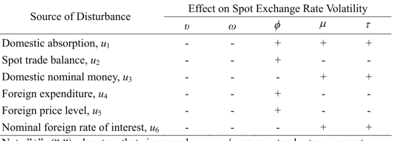
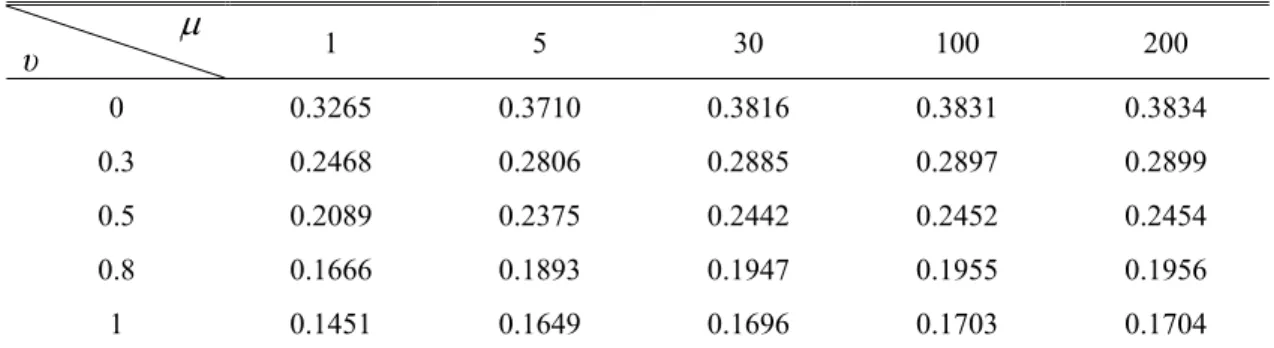
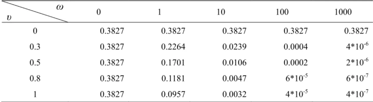
The numerical results for the first part of simulation are presented in Tables 4-8 and summarized in Table 3. It is clear that increase in trader’s sensitivity to central bank’s spot intervention υ tends to stabilize fluctuations of the spot rate in the presence of all disturbances. It is also clear that increase in the preference weight placed by the central bank on reaching the target spot rate ω tends to stabilize

(23)

fluctuations of the spot rate in the presence of all disturbances.12

Increases in the price flexibilityφ tend to stabilize fluctuations of the spot rate if the random disturbance originates in domestic money u3 or foreign interest rate u6.

However, in the presence of domestic absorption disturbance u1, spot trade

disturbance u2, foreign expenditure disturbance u4, or foreign price disturbance u5,

price flexibility tends to be destabilizing. On the contrary, increases in capital mobilityµor speculative elasticityτ tend to stabilize fluctuation of the spot rate in the presence of spot trade disturbance u2, foreign expenditure disturbance u4, or foreign

price disturbance u5. If the random disturbance originates in domestic absorption u1,

domestic money u3, or foreign interest rate u6, capital mobility and speculation tends

to be destabilizing.

Table 3 Summary of Qualitative Results with Base Parameter Values: Spot Rate

Effect on Spot Exchange Rate Volatility Source of Disturbance

υ ω φ µ τ

Domestic absorption, u1 - - + + +

Spot trade balance, u2 - - + - -

Domestic nominal money, u3 - - - + +

Foreign expenditure, u4 - - + - -

Foreign price level, u5 - - + - -

Nominal foreign rate of interest, u6 - - - + +

Note:”+” (“-“) denotes that increased υ, ω,φ , µ orτ tends to augment (dampen)spot rate variability

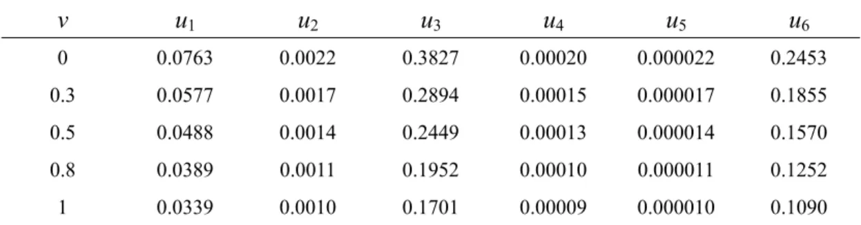
It is also found from Tables 4-8 that domestic monetary disturbance u3 acts as the

main source of spot rate variability, regardless of the degree of υ, ω,φ,µorτ .

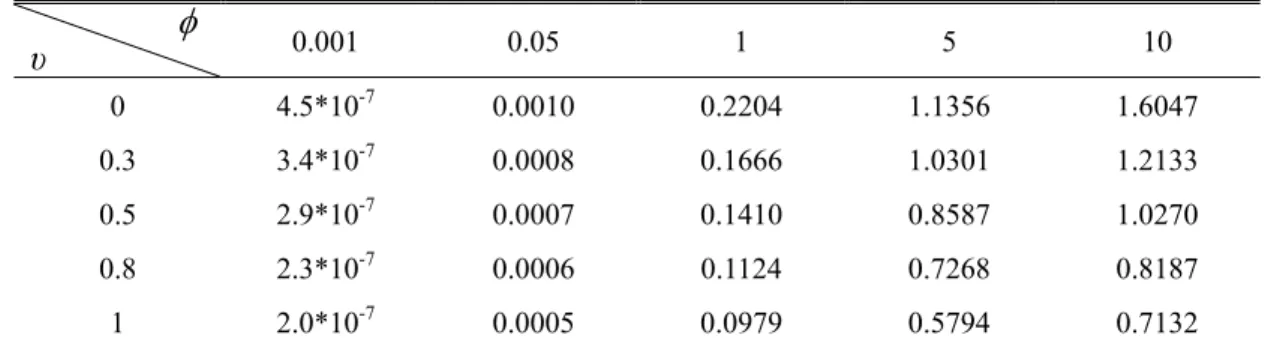
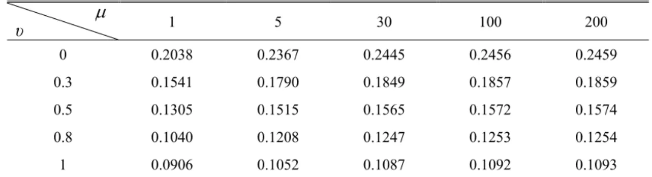
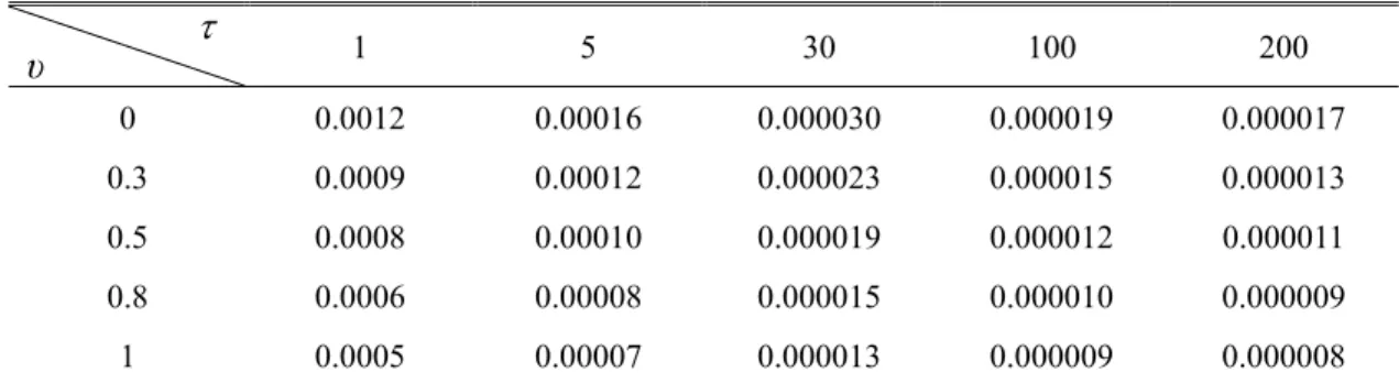
The outcomes of sensitivity analysis are reported in Tables 9-12. All of the tentative conclusions drawn under the base parameter set remain robust. The domestic monetary disturbance u3 remains to be the main source of spot rate variability. In

conclusion, the sensitivity analysis finds that the desirability of central bank spot intervention is generally insensitive to the degree of price flexibility, capital mobility, speculation and central bank’s commitment to the target spot rate.

12_{Increase in υ or ω has the same effect, both in terms of direction and magnitude, on spot exchange}

(24)

Table 4 Variance of Spot Rate under the Base Parameter Set for Different Values of v v u1 u2 u3 u4 u5 u6 0 0.0763 0.0022 0.3827 0.00020 0.000022 0.2453 0.3 0.0577 0.0017 0.2894 0.00015 0.000017 0.1855 0.5 0.0488 0.0014 0.2449 0.00013 0.000014 0.1570 0.8 0.0389 0.0011 0.1952 0.00010 0.000011 0.1252 1 0.0339 0.0010 0.1701 0.00009 0.000010 0.1090

Table 5 Variance of Spot Rate under the Base Parameter Set for Different Values of ω

ω u1 u2 u3 u4 u5 u6 0 0.0763 0.0022 0.3827 0.0002 2.2*10-5 _0.2453 1 0.0339 0.0010 0.1701 9*10-5 _1.0*10-5 _0.1090 10 0.0021 6*10-5 _0.0106 _6*10-6 _6.0*10-7 _0.0068 100 3*10-5 _9*10-7 _0.0002 _8*10-8 _9.0*10-9 _9*10-5 1000 3*10-7 _9*10-9 _2*10-6 _8*10-10 _9.0*10-11 _1*10-6

Table 6 Variance of Spot Rate under the Base Parameter Set for Different Values of φ

φ u1 u2 u3 u4 u5 u6 0.001 2.9*10-7 _{0.0002 0.3573 1.6*10}-5 _1.8*10-6 _0.1589 0.05 0.0007 0.0003 0.3431 2.3*10-5 _2.6*10-6 _0.1587 1 0.1410 0.0030 0.1787 0.00027 0.00003 0.1556 5 0.8587 0.0116 0.0401 0.00100 0.00012 0.1515 10 1.0270 0.0157 0.0157 0.00140 0.00016 0.1501

Table 7 Variance of Spot Rate under the Base Parameter Set for Different Values ofµ

µ _u₁ _u₂ _u₃ _u₄ _u₅ _u₆ 1 0.0354 0.1506 0.2089 0.01360 0.001500 0.1305 5 0.0460 0.0117 0.2375 0.00110 0.000120 0.1515 30 0.0486 0.0020 0.2442 0.00018 0.000020 0.1565 100 0.0490 0.0012 0.2452 0.00011 0.000012 0.1572 200 0.0490 0.0011 0.2454 0.00010 0.000011 0.1574

(25)

Table 8 Variance of Spot Rate under the Base Parameter Set for Different Values of τ τ _u₁ _u₂ _u₃ _u₄ _u₅ _u₆ 1 0.0395 0.0765 0.2201 0.00690 0.000800 0.1386 5 0.0462 0.0103 0.2382 0.00090 0.000100 0.1520 30 0.0486 0.0019 0.2442 0.00017 0.000019 0.1565 100 0.0489 0.0012 0.2452 0.00011 0.000012 0.1572 200 0.0490 0.0011 0.2454 0.00010 0.000011 0.1574

Table 9-1 Variance of Spot Rate against Domestic Absorption Disturbance u1 under

the Sensitivity Analysis: Parameter φ

φ υ 0.001 0.05 1 5 10 0 4.5*10-7 _{0.0010 0.2204 1.1356 1.6047} 0.3 3.4*10-7 _{0.0008 0.1666 1.0301 1.2133} 0.5 2.9*10-7 _{0.0007 0.1410 0.8587 1.0270} 0.8 2.3*10-7 _{0.0006 0.1124 0.7268 0.8187} 1 2.0*10-7 _{0.0005 0.0979 0.5794 0.7132}

Table 9-2 Variance of Spot Rate against Spot Trade Balance Disturbance u2 under the

Sensitivity Analysis: Parameter φ

φ υ 0.001 0.05 1 5 10 0 0.00028 0.00041 0.0047 0.0181 0.0246 0.3 0.00021 0.00031 0.0036 0.0137 0.0186 0.5 0.00018 0.00026 0.0030 0.0116 0.0157 0.8 0.00014 0.00021 0.0024 0.0092 0.0125 1 0.00012 0.00018 0.0021 0.0080 0.0109

Table 9-3 Variance of Spot Rate against Excess Supply of Domestic Nominal Money Disturbance u3 under the Sensitivity Analysis: Parameter φ

φ υ 0.001 0.05 1 5 10 0 0.5583 0.5361 0.2793 0.0626 0.0245 0.3 0.4222 0.4054 0.2112 0.0474 0.0185 0.5 0.3573 0.3431 0.1787 0.0401 0.0157 0.8 0.2849 0.2735 0.1425 0.0320 0.0125 1 0.2481 0.2383 0.1241 0.0278 0.0109

(26)

Table 9-4 Variance of Spot Rate against Foreign Expenditure Disturbance u4 under the

φ υ 0.001 0.05 1 5 10 0 0.000025 0.000037 0.00042 0.0016 0.0022 0.3 0.000019 0.000028 0.00032 0.0012 0.0017 0.5 0.000016 0.000023 0.00027 0.0010 0.0014 0.8 0.000013 0.000019 0.00022 0.0008 0.0011 1 0.000011 0.000016 0.00019 0.0007 0.0010

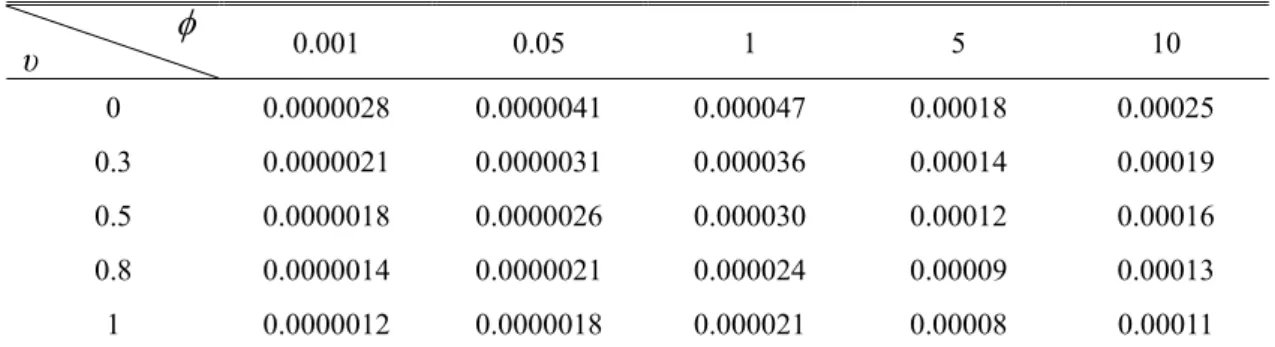
Table 9-5 Variance of Spot Rate against Foreign Price Level Disturbance u5 under the

φ υ 0.001 0.05 1 5 10 0 0.0000028 0.0000041 0.000047 0.00018 0.00025 0.3 0.0000021 0.0000031 0.000036 0.00014 0.00019 0.5 0.0000018 0.0000026 0.000030 0.00012 0.00016 0.8 0.0000014 0.0000021 0.000024 0.00009 0.00013 1 0.0000012 0.0000018 0.000021 0.00008 0.00011

Table 9-6 Variance of Spot Rate against Nominal Foreign Rate of Interest Disturbance u6 under the Sensitivity Analysis: Parameter φ

φ υ 0.001 0.05 1 5 10 0 0.2483 0.2480 0.2432 0.2367 0.2346 0.3 0.1878 0.1875 0.1839 0.1790 0.1774 0.5 0.1589 0.1587 0.1556 0.1515 0.1501 0.8 0.1267 0.1265 0.1241 0.1208 0.1197 1 0.1104 0.1102 0.1081 0.1052 0.1043

the Sensitivity Analysis: Parameter µ

µ υ 1 5 30 100 200 0 0.0554 0.0718 0.0759 0.0765 0.0766 0.3 0.0419 0.0543 0.0574 0.0578 0.0579 0.5 0.0354 0.0460 0.0486 0.0490 0.0490 0.8 0.0282 0.0367 0.0387 0.0390 0.0391 1 0.0246 0.0319 0.0337 0.0340 0.0340

(27)

Sensitivity Analysis: Parameter µ

µ υ 1 5 30 100 200 0 0.2353 0.0183 0.0031 0.0019 0.0017 0.3 0.1779 0.0138 0.0023 0.0015 0.0013 0.5 0.1506 0.0117 0.0020 0.0012 0.0011 0.8 0.1201 0.0093 0.0016 0.0010 0.0009 1 0.1046 0.0081 0.0014 0.0009 0.0008

Table 10-3 Variance of Spot Rate against Excess Supply of Domestic Nominal Money Disturbance u3 under the Sensitivity Analysis: Parameter µ

µ υ 1 5 30 100 200 0 0.3265 0.3710 0.3816 0.3831 0.3834 0.3 0.2468 0.2806 0.2885 0.2897 0.2899 0.5 0.2089 0.2375 0.2442 0.2452 0.2454 0.8 0.1666 0.1893 0.1947 0.1955 0.1956 1 0.1451 0.1649 0.1696 0.1703 0.1704

Table 10-4 Variance of Spot Rate against Foreign Expenditure Disturbance u4 under

µ υ 1 5 30 100 200 0 0.0212 0.0016 0.00027 0.00017 0.00015 0.3 0.0160 0.0012 0.00021 0.00013 0.00012 0.5 0.0136 0.0011 0.00018 0.00011 0.00010 0.8 0.0108 0.0008 0.00014 0.00009 0.00008 1 0.0094 0.0007 0.00012 0.00008 0.00007

Table 10-5 Variance of Spot Rate against Foreign Price Level Disturbance u5 under

µ υ 1 5 30 100 200 0 0.0024 0.00018 0.000031 0.000019 0.000017 0.3 0.0018 0.00014 0.000023 0.000015 0.000013 0.5 0.0015 0.00012 0.000020 0.000012 0.000011 0.8 0.0012 0.00009 0.000016 0.000010 0.000009 1 0.0010 0.00008 0.000014 0.000009 0.000008

(28)

Table 10-6 Variance of Spot Rate against Nominal Foreign Rate of Interest Disturbance u6 under the Sensitivity Analysis: Parameter µ

µ υ 1 5 30 100 200 0 0.2038 0.2367 0.2445 0.2456 0.2459 0.3 0.1541 0.1790 0.1849 0.1857 0.1859 0.5 0.1305 0.1515 0.1565 0.1572 0.1574 0.8 0.1040 0.1208 0.1247 0.1253 0.1254 1 0.0906 0.1052 0.1087 0.1092 0.1093

the Sensitivity Analysis: Parameter τ τ υ 1 5 30 100 200 0 0.0617 0.0723 0.0759 0.0765 0.0766 0.3 0.0466 0.0546 0.0574 0.0578 0.0579 0.5 0.0395 0.0462 0.0486 0.0489 0.0490 0.8 0.0315 0.0369 0.0387 0.0390 0.0391 1 0.0274 0.0321 0.0337 0.0340 0.0340

Sensitivity Analysis: Parameter τ τ υ 1 5 30 100 200 0 0.1195 0.0160 0.0030 0.0019 0.0017 0.3 0.0903 0.0121 0.0023 0.0015 0.0013 0.5 0.0765 0.0103 0.0019 0.0012 0.0011 0.8 0.0610 0.0082 0.0015 0.0010 0.0009 1 0.0531 0.0071 0.0013 0.0009 0.0008

Table 11-3 Variance of Spot Rate against Excess Supply of Domestic Nominal Money Disturbance u3 under the Sensitivity Analysis: Parameter τ

τ υ 1 5 30 100 200 0 0.3439 0.3722 0.3816 0.3831 0.3834 0.3 0.2600 0.2814 0.2886 0.2897 0.2899 0.5 0.2201 0.2382 0.2442 0.2452 0.2454 0.8 0.1754 0.1899 0.1947 0.1955 0.1956 1 0.1528 0.1654 0.1696 0.1703 0.1704

(29)

Table 11-6 Variance of Spot Rate against Nominal Foreign Rate of Interest Disturbance u6 under the Sensitivity Analysis: Parameter τ

τ υ 1 5 30 100 200 0 0.2166 0.2375 0.2445 0.2456 0.2459 0.3 0.1638 0.1796 0.1849 0.1857 0.1859 0.5 0.1386 0.1520 0.1565 0.1572 0.1574 0.8 0.1105 0.1212 0.1248 0.1253 0.1254 1 0.0963 0.1056 0.1087 0.1092 0.1093

the Sensitivity Analysis: Parameter ω ω υ 0 1 10 100 1000 0 0.0763 0.0763 0.0763 0.0763 0.0763 0.3 0.0763 0.0452 0.0048 8*10-5 _8*10-7 0.5 0.0763 0.0339 0.0021 3*10-5 _3*10-7 0.8 0.0763 0.0236 0.0009 1*10-5 _1*10-7 1 0.0763 0.0191 0.0006 7*10-6 _8*10-8

(30)

Sensitivity Analysis: Parameter ω ω υ 0 1 10 100 1000 0 0.0022 0.0022 0.0022 0.0022 0.0022 0.3 0.0022 0.0013 0.0001 2*10-6 _3*10-8 0.5 0.0022 0.0010 6*10-5 _9*10-7 _9*10-9 0.8 0.0022 0.0007 3*10-5 _3*10-7 _3*10-9 1 0.0022 0.0006 2*10-5 _2*10-7 _2*10-9

Table 12-3 Variance of Spot Rate against Excess Supply of Domestic Nominal Money Disturbance u3 under the Sensitivity Analysis: Parameter ω

ω υ 0 1 10 100 1000 0 0.3827 0.3827 0.3827 0.3827 0.3827 0.3 0.3827 0.2264 0.0239 0.0004 4*10-6 0.5 0.3827 0.1701 0.0106 0.0002 2*10-6 0.8 0.3827 0.1181 0.0047 6*10-5 _6*10-7 1 0.3827 0.0957 0.0032 4*10-5 _4*10-7

the Sensitivity Analysis: Parameter ω ω υ 0 1 10 100 1000 0 0.0002 0.0002 0.0002 0.0002 0.0002 0.3 0.0002 0.0001 0.0001 2*10-7 _2*10-9 0.5 0.0002 9*10-5 _6*10-6 _8*10-8 _8*10-10 0.8 0.0002 6*10-5 _3*10-6 _3*10-8 _3*10-10 1 0.0002 5*10-5 _2*10-6 _2*10-8 _2*10-10

the Sensitivity Analysis: Parameter ω ω υ 0 1 10 100 1000 0 2.2*10-5 _2.2*10-5 _2.2*10-5 _2.2*10-5 _2.2*10-5 0.3 2.2*10-5 _1.3*10-5 _1.4*10-6 _2.3*10-8 _2.5*10-10 0.5 2.2*10-5 _1.0*10-5 _6.0*10-7 _9.0*10-9 _9.0*10-11 0.8 2.2*10-5 _7.0*10-6 _3.0*10-7 _3.0*10-9 _3.0*10-11 1 2.2*10-5 _6.0*10-6 _2.0*10-7 _2.0*10-9 _2.0*10-11

(31)

Table 12-6 Variance of Spot Rate against Nominal Foreign Rate of Interest Disturbance u6 under the Sensitivity Analysis: Parameter ω

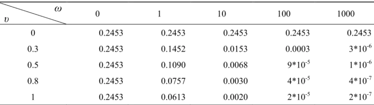
ω υ 0 1 10 100 1000 0 0.2453 0.2453 0.2453 0.2453 0.2453 0.3 0.2453 0.1452 0.0153 0.0003 3*10-6 0.5 0.2453 0.1090 0.0068 9*10-5 _1*10-6 0.8 0.2453 0.0757 0.0030 4*10-5 _4*10-7 1 0.2453 0.0613 0.0020 2*10-5 _2*10-7

Numerical Simulation in the Case of Forward Market Intervention

Given the base parameter set, the first part of the numerical simulation is conducted by allowing ζ which measures trader’s sensitivity to central bank’s forward intervention to vary from 0 to 1. The degree of the forward rate variability measured by equation (30b) is calculated for each given value of ζ, given other parameters held at their base values. The same procedure is applied to ρ,φ,µandτ . The second part is sensitivity analysis, in which given other parameters held constant, the degree of the forward rate variability is calculated for each possible combination of ζ andφ, ζ andµ, ζ andτ as well as ζ and ρ.

The numerical results for the first part of simulation are presented in Tables 14-18 and summarized in Table 13. It is clear that increase in trader’s sensitivity to central bank’s forward intervention tends to stabilize fluctuations of the forward rate in the presence of all disturbances. It is also clear that increase in the preference weight placed by the central bank on reaching the target forward rate tends to stabilize fluctuations of the forward rate in the presence of all disturbances.13

Increases in price flexibilityφtend to stabilize fluctuations of the forward rate if the random disturbance originates in spot trade u2, foreign expenditure u4, foreign

price u5 or foreign interest rate u6, but tends to be destabilizing if the random

disturbance originates in domestic absorption u1. However, in the presence of

domestic money disturbance u3, price flexibility may be stabilizing if the degree of

price flexibility is low or destabilizing if degree of price flexibility is high. Increase in capital mobilityµclearly destabilizes the fluctuation of forward rate in the presence of all disturbances. On the contrary, increase in speculative elasticityτ clearly stabilizes the fluctuation of forward rate in the presence of all disturbances. It should be noted that in most cases, whether stabilizing or destabilizing, each parameter ξ,

13_{Increase in ξ or ρ has the same effect, both in terms of direction and magnitude, on spot exchange}

(32)

ρ,φ,µorτ has only a rather minor effect on the volatility of the forward rate.

The outcomes of sensitivity analysis are reported in Tables 19-22. All of the tentative conclusions drawn under the base parameter set remain robust. In conclusion, the sensitivity analysis finds that the desirability of central bank forward intervention is generally insensitive to the degree of price flexibility, capital mobility, speculation and central bank’s commitment to the target forward rate.

Table 13 Summary of Qualitative Results with Base Parameter Values: Forward Rate

Effect on Spot Exchange Rate Volatility Source of Disturbance

ξ ρ φ µ τ

Domestic absorption, u1 - - + + -

Spot trade balance, u2 - - - + -

Domestic nominal money, u3 - - - or + + -

Foreign expenditure, u4 - - - + -

Foreign price level, u5 - - - + -

Nominal foreign rate of interest, u6 - - - + -

Note:”+” (“-“) denotes that increased ξ, ρ,φ ,µorτ tends to augment (dampen) forward rate variability.

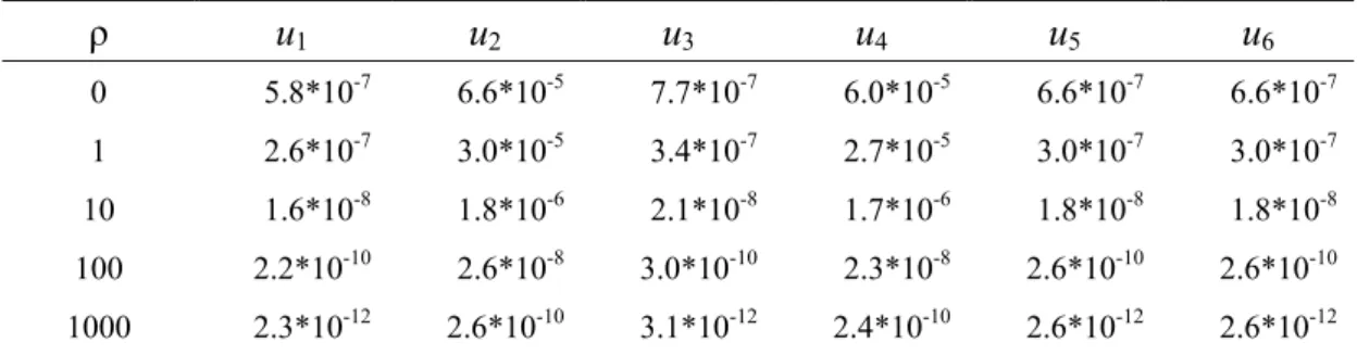
Table 14 Variance of Forward Rate under the Base Parameter Set for Different values of ξ ξ u1 u2 u3 u4 u5 u6 0 5.8*10-7 _{0.000066 7.7*10}-7 _{0.000060 6.6*10}-7 _6.6*10-7 0.3 4.4*10-7 _{0.000050 5.8*10}-7 _{0.000045 5.0*10}-7 _5.0*10-7 0.5 3.7*10-7 _{0.000043 4.9*10}-7 _{0.000038 4.3*10}-7 _4.3*10-7 0.8 3.0*10-7 _{0.000034 3.9*10}-7 _{0.000031 3.4*10}-7 _3.4*10-7 1 2.6*10-7 _{0.000030 3.4*10}-7 _{0.000027 3.0*10}-7 _3.0*10-7

(33)

Table 15 Variance of Forward Rate under the Base Parameter Set for Different Values of ρ ρ u1 u2 u3 u4 u5 u6 0 5.8*10-7 _6.6*10-5 _7.7*10-7 _6.0*10-5 _6.6*10-7 _6.6*10-7 1 2.6*10-7 _3.0*10-5 _3.4*10-7 _2.7*10-5 _3.0*10-7 _3.0*10-7 10 1.6*10-8 _1.8*10-6 _2.1*10-8 _1.7*10-6 _1.8*10-8 _1.8*10-8 100 2.2*10-10 _2.6*10-8 _3.0*10-10 _2.3*10-8 _2.6*10-10 _2.6*10-10 1000 2.3*10-12 _2.6*10-10 _3.1*10-12 _2.4*10-10 _2.6*10-12 _2.6*10-12

Table 16 Variance of Forward Rate under the Base Parameter Set for Different Values of φ φ u1 u2 u3 u4 u5 u6 0.001 2.2*10-12 _{0.000043 1.0*10}-6 _3.9*10-6 _4.3*10-7 _4.3*10-7 0.05 5.3*10-9 _{0.000043 9.0*10}-7 _3.9*10-6 _4.3*10-7 _4.3*10-7 1 1.1*10-6 _{0.000042 2.5*10}-7 _3.8*10-6 _4.2*10-7 _4.2*10-7 5 5.5*10-6 _{0.000040 1.2*10}-8 _3.6*10-6 _4.0*10-7 _4.0*10-7 10 7.8*10-6 _{0.000039 1.0*10}-6 _3.5*10-6 _3.9*10-7 _3.9*10-7

Table 17 Variance of Forward Rate under the Base Parameter Set for Different Values of µ µ _u₁ _u₂ _u₃ _u₄ _u₅ _u₆ 1 3.1*10-7 _{0.000035 4.1*10}-7 _3.2*10-6 _3.5*10-7 _3.5*10-7 5 3.6*10-7 _{0.000041 4.8*10}-7 _3.7*10-6 _4.1*10-7 _4.1*10-7 30 3.7*10-7 _{0.000042 4.9*10}-7 _3.8*10-6 _4.2*10-7 _4.2*10-7 100 3.7*10-7 _{0.000043 5.0*10}-7 _3.8*10-6 _4.3*10-7 _4.3*10-7 200 3.7*10-7 _{0.000043 5.0*10}-7 _3.8*10-6 _4.3*10-7 _4.3*10-7

Table 18 Variance of Forward Rate under the Base Parameter Set for Different Values of τ τ _u₁ _u₂ _u₃ _u₄ _u₅ _u₆ 1 0.00053 0.0611 0.00070 0.0055 0.00060 0.00060 5 0.00004 0.0050 0.00006 0.0005 0.00005 0.00005 30 1.5*10-6 _{0.0002 1.9*10}-6 _1.5*10-5 _1.7*10-6 _1.7*10-6 100 1.4*10-6 _1.5*10-5 _1.8*10-7 _1.4*10-6 _1.5*10-7 _1.5*10-7 200 3.4*10-8 _3.9*10-6 _4.5*10-8 _3.5*10-7 _3.9*10-8 _3.9*10-8

匯率波動性與中央銀行最適干預

行政院國家科學委員會專題研究計畫 成果報告