Bridge-connectivity Augmenting Problem with a
Partition Constraint
Hsin-Wen Wei
∗, Wan-Chen Lu
†, Pei-Chi Huang
†, Wei-Kuan Shih
†, and Tsan-sheng Hsu
∗ ∗Institute of Information Science, Academia Sinica, Nankang, Taipei, Taiwan
{hwwei, tshsu}@iis.sinica.edu.tw
†
Department of Computer Science, National Tsing-Hua University, Hsinchu, Taiwan
{wanchen, peggy, wshih}@rtlab.cs.nthu.edu.tw
Abstract
This paper considers the augmentation problem of an undirected graph with k partitions of its vertices. The main issue is how to add a set of edges with the smallest possible cardinality so that the resulting graph is 2-edge-connected, i.e., bridge-connected, while maintaining the partition constraint. To solve this problem, we propose a simple linear-time algo-rithm. We show that the algorithm runs in O(log n) parallel time on an EREW PRAM using a linear number of processors.
Key words: 2-edge-connectivity, bridge-connectivity, augmentation, partition constraint
1
Introduction
A graph is said to be k-edge-connected if it remains connected after the removal of any set of edges whose cardinality is less than k. Finding the smallest set of edges to make an undirected graph k-edge-connected is a fundamental problem in many important appli-cations; readers may refer to [4, 7, 12] for a com-prehensive survey. Many algorithms have been devel-oped to resolve the problem of making general graphs k-edge connected or k-vertex connected for various values of k [3, 8, 9, 10, 14, 17]. Note that there is a linear-time algorithm for the smallest bridge-connectivity augmentation problem on the general graph that does not have a partition constraint [3]. In [6], a linear-time algorithm for bridge-connectivity augmentation with a bipartite constraint is described. In [11], Jensen et al. proposed a polynomial time al-gorithm that solves the k-edge-connectivity augmenta-tion problem on a graph that has partiaugmenta-tion constraints in O(n(m+n log n) log n) time, where m is the number of distinct edges in the input graph.
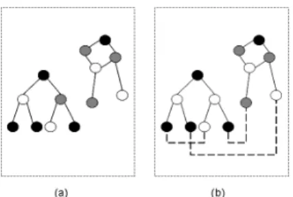
Figure 1: (a) A graph with three partitions of vertices. (b) A smallest 2-edge-connectivity augmentation of (a) with the set of added edges marked by dashed lines.
In this paper, we focus on augmenting graphs with a partition constraint. Here the partition constraint is that the vertex set of an input graph is parti-tioned into k disjoint vertex subsets and each edge in the augmentation must be added between two dif-ferent vertex subsets. We propose a linear-time algo-rithm that addresses the problem of adding the small-est number of edges to a given graph with a given partition constraint to make it 2-edge-connected, or bridge-connected, while maintaining the constraint. Figure 1(a) shows an example of a graph with three partitions of vertices. A smallest 2-edge-connectivity augmentation of Figure 1(a) is shown in Figure 1(b).
We solve the problem of a smallest 2-edge-connectivity augmentation of graphs with a partition constraint by transforming the input graph G into a well-known data structure called a bridge-block for-est [5]. Our approach adds the smallfor-est possible num-ber of edges to make a bridge-block forest 2-edge-connected. Note that the edge set added to the bridge-block forest by our algorithm can be transformed into the corresponding edge set added to the input graph G. The algorithm runs in sequential liner time and O(log n) parallel time on an EREW PRAM using a linear number of processors.
The remainder of this paper is organized as fol-lows. Section 2 contains graph-theoretical definitions and previously known properties. In Section 3, we in-troduce the concept of loose edges and propose an al-gorithm that makes a loose forest 2-edge-connected. In Section 4, we propose an algorithm that finds a small-est 2-edge-connectivity augmentation for a bridge-block forest. The paper is concluded in Section 5.
2
Preliminaries
2.1
Graph-theoretical definitions
Let a graph G = (V, E), where |V | = n and |E| = m. G is a tree if it is an undirected, connected, and acyclic graph. A maximal connected subgraph is a component of G. A forest is a graph, whose components are all trees, and a degree-1 vertex of a forest is called a leaf. An edge whose endpoints are a vertex u and a vertex v is denoted as (u, v). Note that, for an edge set E0,
G − E0 denotes G without the edges in E0, and G ∪ E0
denotes G with the edges in E0
added to it.
In this paper, all graphs are undirected, and have neither self-loops nor multiple edges. The vertex set of an input graph is assumed to be partitioned into k disjoint partitions. A partition of the vertex set in a graph is called a vertex partition. Let Pi denote the
ith vertex partition of an input graph, i.e., Pi is a
subset of V , and V = {P1∪ P2∪ · · · ∪ Pk} (k ≥ 1),
∀Pi, Pj ∈ V , Pi∩ Pj = ∅, i 6= j. Our problem is how
to add a set of edges such that the resulting graph is 2-edge-connected and the two endpoints of each added edge are not in the same vertex partition.
2.2
Bridge-block forest
A vertex u is connected to a vertex v in a graph G if u and v are in the same connected component of G. Two vertices of a graph are 2-edge-connected if they are in the same connected component and remain so after the removal of any single edge. A set of vertices is connected if each pair of its vertices is 2-edge-connected; similarly, a graph is 2-edge-connected if its set of vertices is 2-edge-connected. A bridge is an edge of a graph G, the removal of which would increase the number of connected components of G by one. Given a graph G with at least three vertices, a smallest 2-edge-connectivity augmentation of G, denoted by aug2e(G), is a set of edges with the minimum cardinality whose addition makes G 2-edge-connected.
A block in a graph is an induced subgraph of a max-imal 2-edge-connected subset of vertices. If a block contains all the nodes in a connected component of
G, it is called an isolated block. A singular connected component is one formed by an isolated vertex, and a singular block is one with exactly one vertex. The bridge-block graph of an undirected graph G, denoted by BB(G), is defined as follows. Each block is repre-sented by a vertex of BB(G). When all the blocks in G are represented by vertices, BB(G) becomes a for-est, such that each bridge in G corresponds to an edge in BB(G) and vice versa. For example, the blocks a, b, · · · , i are represented by vertices. The resulting tree is illustrated in Figure 2. A mono block of Pi in
G is a block comprised of vertices in Piof G. A hybrid
block in G is a block containing at least two vertices, one in Pi and another in Pj of G, where i 6= j and
Pi, Pj ∈ V . An isolated mono block of Pi in G is an
isolated block and also a mono block of Pi in G. An
isolated hybrid block in G is an isolated block and also a hybrid block in G.
The vertices and leaves in BB(G) are defined as follows. Given a graph G with k vertex partitions P1, · · · , Pk, k ≥ 1, let Ci denote the ith vertex
par-tition in BB(G), where all corresponding blocks and vertices are in Pi of G. An isolated vertex of Ci in
BB(G) is an isolated mono block of Pi or an isolated
vertex of Pi in G. An isolated hybrid vertex in BB(G)
is an isolated hybrid block in G. A mono leaf (respec-tively, mono vertex) of Ci in BB(G) is a leaf
(respec-tively, vertex) in BB(G), whose corresponding block in G is a mono block of Pi. A hybrid leaf in BB(G) is
a vertex in BB(G), whose corresponding block in G is a hybrid block.
In addition, let Fn be a function that can trans-form an edge set added to BB(G) into a correspond-ing edge set added to G. If E0 is the edge set added
to BB(G), then Fn(E0
) is the corresponding edge set added to G, i.e., aug2e(G)=Fn(E0). Similarly, if e0
is an edge added to BB(G), then Fn(e0) is a
corre-sponding edge added between a black vertex and a non-adjacent white vertex of G, if possible.
Given a PRAM model M, let TM(n, m) be the
parallel time needed to compute the connected com-ponents of G using PM(n, m) ≤ (n + m) processors.
Fact 1 ([1, 2])
1. If M = CRCW , then TCRCW(n, m) =
O(log n) and PCRCW(n, m) =
O((n + m)·α(m, n)/ log n).
2. If M = EREW , then TEREW(n, m) = O(log n)
and PEREW(n, m) = O(n + m).
A rooted bridge-block forest for a graph can be computed in sequential linear time and in O(log n + TM(n, m)) parallel time using O((n + m)/ log n +
Figure 2: (a) A graph has three vertex partitions and the maximum 2-edge-connected subsets of vertices of this graph are grouped into a set of blocks by the dashed lines. (b) The bridge-block forest of the graph in (a).
Fact 2 An edge can be added between two blocks in G, unless both blocks are mono blocks of Pi in G.
3
Loose Forest
To reduce the complexity of finding the augmentation of a graph, we introduce a new concept of loose edges. If an edge e = (u, v) with two endpoints u and v in different vertex partitions of G, i.e., u ∈ Pi, v ∈ Pj, i 6=
j, can be removed from the input graph G and its two endpoints u, v can be connected to other vertices in G, then this edge is called a loose edge. Conversely, if an edge is not a loose edge, it is called a fixed edge. A loose block of a graph is the induced subgraph of the maximal 2-edge-connected subset of vertices and contains exactly one loose edge. A bridge-block tree is loose if each leaf in the tree is a loose block. A bridge-block forest is defined as a loose forest, if all of its trees are loose trees.
In this paper, we first solve the problem of making a loose forest 2-edge-connected. We then solve the prob-lem of a smallest 2-edge-connectivity augmentation of a graph with a partition constraint by transforming the input graph G into a loose forest. For simplifying the discussion, we define two operations reconnect and swap. Reconnect is an operation that removes a set of edges Er from the given graph or data structure and
adds a set of edges Ea, which connect the endpoints of
the removed edges, where |Er| = |Ea| and Er∩Ea= ∅.
Let e1 = (u1, v1), e2= (u2, v1) be two edges, swap e1
and e2 is an operation that removes e1, e2 and adds
two edges e0
1= (u1, v2), e02= (u1, v1) or e01= (u1, u2),
e0
2= (v1, v1). The following lemma shows the property
of swap operation.
Lemma 1 (swap property) Given two
2-edge-connected components G1 and G2, and two edges e1, e2, where e1 = (u1, v1) ∈ G1, e2 = (u2, v2) ∈ G2. Let G0 = G 1∪ G2− {e1, e2} ∪ (u1, v2) ∪ (u2, v1) or G0 = G 1∪ G2− {e1, e2} ∪ (u1, u2) ∪ (v1, v2), then G0 is a 2-edge-connected component.
Proof. After removing e1 (respectively, e2), there is still a tree path from u1 to v1 in G1 (respectively, from u2 to v2in G2). After adding edges (u1, v2) and (u2, v1) (or (u1, u2) and (v1, v2)), then G1and G2 are connected, and it is obvious that there exists a cycle containing (u1, v1, u2, v2). Therefore G0 is a
2-edge-connected component. 2
Before solving the case of loose forest, we first con-sider a simpler case that takes a set of loose blocks as an input graph. We propose an method that reconnets a set of loose blocks to a 2-edge-connected component as shown in Algorithm 1.
Algorithm 1 Reconnect a set of loose blocks to a 2-edge-connected component
1: procedure LBto2EC(LB, EL) {∗ LB is a set of
loose blocks with a set of loose edges ELin it ∗}
2: E0= ∅; EL0 = ∅; LB0= LB
3: Number each loose block in LB as b1, · · · , b|LB|;
4: Number the loose edge in the loose block bi as ei,
1 ≤ i ≤ |EL|; {∗ |LB| = |EL| ∗}
5: if there are at least two loose blocks in LB0 then 6: fori from 1 to bEL/2c do
7: LB0= LB0− e2i−1− e2i; {∗ Assume that
e2i−1= (a, b) and e2i= (c, d); ∗}
8: if a and c are in the same vertex partition
or b and d are in the same vertex par-tition then
9: Let e01= (a, d) and e02= (b, c);
10: else
11: Let e01= (a, c) and e02= (b, d); 12: end if
13: Let e01 be a loose edge and e02 be a fixed
edge; 14: LB0= LB0∪ e01∪ e02; 15: E0 L= EL0 ∪ e01; 16: E0= E0∪ e02; 17: end for 18: if |EL| is odd then 19: Let EL0 = EL0 ∪ e|E L|; 20: end if 21: Let E0= E0∪ LBto2EC(LB0, EL0); 22: end if 23: returnE0; 24: end procedure
Lemma 2 Let BB(G) be the input graph and EL be
E0 is a 2-edge-connected compoent, where E0 is the
edge set that returned by Algorithm 1, and no edges in E0 violate the partition constraint.
Proof. By Lemma 1, two loose blocks can be recon-nected to a 2-edge-conrecon-nected component after swap-ping their loose edges. Note that steps 7 − 14 process swap operation between two loose edges. In addition, one of the new edges formed by swap operation in the new block is assigned as a loose edge and the other edge is assigned fixed. The new formed block is also a loose block. Since our algorithm recursively swaps loose edges between two loose blocks until there is only one loose block, the set of loose blocks is reconnected to a 2-edge-connected component.
Now, we consider whether the edges in E0
violate the partition constraint. In our algorithm, it swaps two loose edges e2i−1 = (a, b), e2i= (c, d) of two loose
blocks. Since a loose edge connects two vertices in different partitions, then a (respectively, c) and b (re-spectively, d) are in different partitions, In addition, it is obvious to see that the partition constraint of these added edges can be guaranteed by steps 8−12. There-fore, no edges in E0
violate the partition constraint. 2 Now, we consider a loose forest F as an input graph, it is trivial to see that Algorithm 2 can cor-rectly reconnect a loose forest to a 2-edge-connected component.
Algorithm 2 Reconnect a loose forest to a 2-edge-connected component
1: procedure Fto2EC(F , EL) {∗ F is a loose forest
with a set of loose edges EL. ∗}
2: E0= ∅;
3: Let X be a set of leaves and isolated vertices in F ; 4: E0=LBTo2EC(X,EL);
5: returnE0; 6: end procedure
4
Main Result
Let G be the input graph. In this paper, we use F and BB(G) interchangeably to denote the bridge-block forest for an input graph G. C1, C2, · · · , Ckdenote the
vertex partitions of BB(G). Let Si and H denote the
sets of mono leaves of Ci and a set of hybrid leaves
in BB(G), respectively. In addition, let S∗
i and H
∗
denote the sets of isolated vertices of Ci and a set of
isolated hybrid vertices in BB(G), respectively. We say that BB(G) is Ci-dominated if |Si| + 2|Si∗| > d(2|S ∗ 1| + · · · + 2|S∗ k| + 2|H ∗| + |S 1| + · · · + |Sk| + |H|)/2e.
Let | ˆSmax| = max{|Si|+2|Si∗||1 ≤ i ≤ k}. Without
loss of generality, we assume that |S1|+2|S∗1| = | ˆSmax|.
4.1
Lower bound on
aug2e(BB(G))
Let LOWi2e(BB(G)) = max{| ˆSmax|, d(2|S1∗| + · · · +
2|S∗ k| + 2|H
∗| + |S
1| + · · · + |Sk| + |H|)/2e}.
Theorem 1 |aug2e(BB(G))| ≥ LOWi2e(BB(G)).
Proof. Note that each leaf needs one incident edge and each isolated vertex needs two incident edges to make the resulting graph 2-edge-connected. Hence, |aug2e(G)| ≥ d(2|S∗ 1| + · · · + 2|S ∗ k| + 2|H ∗| + |S 1| +
· · · + |Sk| + |H|)/2e. By Fact 2, the endpoints of an
added edge cannot both be in the same vertex par-tition. Thus, |aug2e(G)| ≥ | ˆSmax|, so the theorem
holds. 2
Corollary 1 If BB(G) is Ci-dominated, then
LOWi2e(BB(G)) = |Si| + 2|Si∗|.
Proof. By definition. 2
4.2
Augmentation Algorithm
First, we present an algorithm that numbers the leaves and isolated vertices of an input bridge-block forest, as shown in Algorithm 3. Based on the assigned num-bers of leaves and isolated vertices, we can add edges between the leaves and isolated vertices of the in-put graph without violating the partition constraint. Then, we present an algorithm for finding the aug-mentation of BB(G), as shown in Algorithm 4. Here we assume that, BB(G) contains at least two leaves or two isolated vertices, or at least one leave and one isolated vertex that are in different vertex partitions Algorithm 3 Numbering the leaves and isolated ver-tices in F
1: procedure Numbering(F ) {∗ F is a bridge-block
forest with k partitions of its vertices; ∗}
2: Let λ0= 0;
3: fori from 1 to k do
4: Assign a number to each leaf in Sifrom λi−1+1
to λi−1+ |Si|;
5: Assign two consecutive numbers to each
iso-lated vertex in S∗ i,
from λi−1+|Si|+1 to λi−1+|Si|+2|Si∗|;
6: Let λi= λi−1+ |Si| + 2|Si∗|; 7: end for
8: Assign a number to each leaf in H from λk+ 1 to
λk+ |H|;
9: Assign two consecutive numbers to each isolated
vertex in H∗, from λ
k+ |H| + 1 to λk+ |H| +
2|H∗|;
10: end procedure
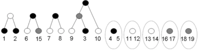
Figure 3 illustrate the numbering procedure in Al-gorithm 3. In this example, there are three vertex
Figure 3: An illustration of the Numbering Procedure. partitions. The black, white, and gray circles denote the vertices of the first, second, and third partitions, respectively. The black leaves in the graph are num-bered 1 to 3 and each isolated vertex is assigned two consecutive numbers; therefore, the black isolated ver-tices are numbered 4 and 5. Similarly, the verver-tices of the second and third partitions are assigned consecu-tive numbers.
Lemma 3 The partition constraint is maintained in Algorithm 4.
Proof. According to Algorithm 3, the vertices in the same vertex partition are assigned successive num-bers, and the numbers assigned to a vertex parti-tion are equal to |Si| + 2|S∗i|, 1 ≤ i ≤ k. We
prove the lemma with the following cases. Note that, |S1| + 2|S∗
1| = | ˆSmax| . In case 1, | ˆSmax| is less than
b`/2c. Since | ˆSmax| = max{|Si| + 2|Si∗||1 ≤ i ≤ k},
no vertex partition is assigned more than `/2 numbers if ` is even; and no vertex partition is assigned more than b`/2c numbers if ` is odd.
Case 1.1: ` is even. The algorithm only adds an edge between two vertices with numbers i and i + `/2, 1 ≤ i ≤ `/2. If two vertices with numbers i and i + `/2 are in the same vertex partition, then the vertex partition must contain `/2 + 1 numbers. However, since no vertex partition is assigned more than `/2 numbers, a vertex partition can not have two vertices with numbers i and i + `/2.
Case 1.2: ` is odd. The algorithm adds an edge between two vertices with numbers i and i + b`/2c, 1 ≤ i ≤ b`/2c, and two vertices with numbers b`/2c+1 and `. If two vertices with numbers i and i + b`/2c or b`/2c + 1 and ` are in the same vertex partition, then the vertex partition must contain b`/2c + 1 numbers. However, since no vertex partition is assigned more than b`/2c numbers, a vertex partition can not have two vertices with numbers i and i + b`/2c.
Case 2: | ˆSmax| > b`/2c. Clearly, the algorithm
only adds edges between the vertex partition that has | ˆSmax| numbers and other vertex partitions. Therefore
the lemma holds. 2
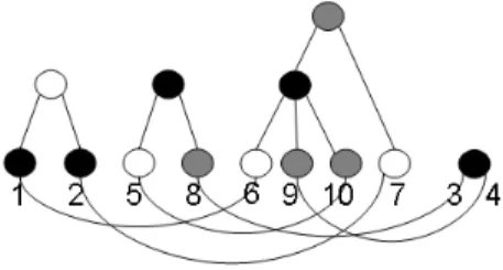
Figure 4 shows an example that illustrates steps
5 − 15 of Algorithm 4.
Theorem 2 Algorithm 4 is correct and optimal. Proof. We first prove the correctness of Algorithm 4. In step 5, the algorithm applies Algorithm 3 to assign numbers to leaves and isolated vertices. By Lemma 3, the partition constraint is maintained after adding edges. Steps 16 − 21, transform a graph into a loose forest. Then, in step 22, the algorithm applies Al-gorithm 2 to reconnect the loose forest into a single 2-edge-connected component. Therefore, Algorithm 4 is correct.
Next, we prove the optimality of our algorithm, which must consider two cases: case 1, | ˆSmax| ≤ b`/2c,
and case 2. | ˆSmax| > b`/2c. It is obvious that the
number of edges added in case 1 is equal to d`/2e in steps 8 − 12 of the algorithm. Therefore, the number of added edges in case 1 is equal to LOWi2e(BB(G)).
Similarly, the number of added edges in case 2 is equal to | ˆSmax| and | ˆSmax| > b`/2c, i.e., Smaxˆ -dominated.
The number of added edges in case 2 is also equal to LOWi2e(BB(G)). Note that the algorithm does not add any edges in steps 16−20. Therefore, Algorithm 4
is optimal. 2
Theorem 3 Algorithm 4 runs in sequential linear time and O(log n) parallel time on an EREW PRAM using a linear number of processors.
Proof. Given a graph G as input, by Fact 1,
the first step in Algorithm 4 takes sequential lin-ear time and O(log n + TM(n, m)) parallel time using
O((n+m)/ log n+PM(n, m)) processors on an EREW
PRAM to compute BB(G). After computing BB(G), the numbering procedure takes sequential liner time and O(log n) parallel time. Then, the algorithm takes O(1) time to determine which case should be executed. In steps 7 − 19, the algorithm takes sequential liner time and O(log n) parallel time to add edges between vertices. Finally, the algorithm applies Algorithm 2 to reconnect the graph to a 2-edge-connected compo-nent, and it is obvious that Algorithm 2 takes sequen-tial liner time O(log n) parallel time. Therefore, this
theorem holds. 2
Note, it is clear that the resulting graph derived by Algorithm 4 is a simple graph, since the algorithm only adds edges between leaves and isolated vertices, and no edge would be added between a vertex and its parent.
5
Concluding remarks
We have proposed a number of algorithms for find-ing a smallest 2-edge-connectivity augmentation of
in-Algorithm 4 Finding a smallest 2-edge-connectivity augmentation of a graph G with a partition constraint
1: procedure FS2Aug(G) 2: Let F = BB(G); 3: Let ` =Pk i=1|Si| + 2|S ∗ i| + |H| + 2|H∗|; 4: E = ∅; E0= ∅; E1= ∅; E2= ∅; 5: Numbering(F ); 6: switch(| ˆSmax|) 7: Case 1: | ˆSmax| ≤ b`/2c 8: Case 1.1: ` is even 9: E0= {(vi, vi+`/2)|1 ≤ i ≤ `/2}; 10: Case 1.2: ` is odd 11: E0= {(vi, vi+b`/2c)|1 ≤ i ≤ b`/2c}; 12: E1= {vb`/2c, v`}; 13: Case 2: | ˆSmax| > b`/2c 14: E0= {(vi, v
i+|Smaxˆ |)|1 ≤ i ≤ ` − | ˆSmax|};
15: E1= {(vj, v`)|` − | ˆSmax| + 1 ≤ j ≤ | ˆSmax|};
16: Let E0= E0∪ E1; 17: Let F0= BB(F ∪ E0);
18: Let X be a set of leaves and isolated vertices in F0; 19: Arbitrarily select an added edge in each leaf and
each isolated vertex of F0from E0and let E2=
e1, e2, · · · , e|X| denote the set of the selected
added edges;
20: E0= E0− E2;
21: Let all edges in E2 be loose edges;
22: E2=FTo2EC(F0, E2); 23: E = E0∪ E2;
24: returnE;
25: end procedure
put graphs with a partition constraint. The proposed methods produce a simple graph if possible, or a multi-graph when it is not possible to obtain a simple multi-graph by any approach. The algorithms can be trivially par-allelized to run in optimal O(log n) time using a linear number of EREW processors.
References
[1] K. W. Chong, Y Han, and T. W. Lam. Concurrent threads and optimal parallel minimum spanning trees algorithm. Journal of ACM, 48(2):297–323, 2001. [2] R. Cole and U. Vishkin. Approximate parallel
scheduling. Part II: Applications to logarithmic-time optimal graph algorithms. Information and Compu-tation, 92:1–47, 1991.
[3] K. P. Eswaran and R. E. Tarjan. Augmentation prob-lems. SIAM Journal on Computing, 5:653–665, 1976. [4] A. Frank. Connectivity augmentation problems in network design. In J. R. Birge and K. G. Murty, ed-itors, Mathematical Programming: State of the Art 1994, pages 34–63. The University of Michigan, 1994.
Figure 4: An illustration of steps in Algorithm 4.
[5] F. Harary. Graph Theory. Addison-Wesley, Reading, Massachusetts, 1969.
[6] P. C. Huang, H. W. Wei, W. C. Lu, W. K. Shih, and T.-s. Hsu. Smallest Bipartite Bridge-connectivity Augmentation. Algorithmica, 2007.
[7] T.-s. Hsu. Graph Augmentation and Related Prob-lems: Theory and Practice. PhD thesis, University of Texas at Austin, 1993.
[8] T.-s. Hsu. On four-connecting a triconnected graph. Journal of Algorithms, 35:202–234, 2000.
[9] T.-s. Hsu. Simpler and faster biconnectivity augmen-tation. Journal of Algorithms, 45(1):55–71, 2002. [10] T.-s. Hsu and M. Y. Kao. Optimal augmentation for
bipartite componentwise biconnectivity in linear time. SIAM Journal on Discrete Mathematics, 19(2):345– 362, 2005.
[11] J. B. Jensen, H. N. Gabow, T. Jordan, and Z. Szigeti. Edge-connectivity augmentation with partition con-straints. SIAM Journal on Discrete Mathematics, 12:160–207, 1999.
[12] H. Nagamochi. Recent development of graph connec-tivity augmentation algorithms. IEICE Transactions on Information and System, E83-D:372–383, 2000. [13] V. Ramachandran. Parallel open ear decomposition
with applications to graph biconnectivity and tricon-nectivity. In J. H. Reif, editor, Synthesis of Parallel Algorithms, pages 275–340. Morgan-Kaufmann, 1993. [14] A. Rosenthal and A. Goldner. Smallest augmentations to biconnect a graph. SIAM Journal on Computing, 6:55–66, 1977.
[15] R. E. Tarjan. Depth-first search and linear graph al-gorithms. SIAM Journal on Computing, 1:146–160, 1972.
[16] R. E. Tarjan and U. Vishkin. An efficient parallel bi-connectivity algorithm. SIAM Journal on Computing, 14:862–874, 1985.
[17] T. Watanabe and A. Nakamura. A minimum 3-connectivity augmentation of a graph. Journal of Computer and System Science, 46:91–128, 1993.