應用混合啟發式演算法推估地下水污染物暫態釋放問題

國 立 交 通 大 學

環 境 工 程 研 究 所

碩 士 論 文

應用混合啟發式演算法推估地下水污染物暫態釋放問題

Apply Hybrid Heuristic Approach to Identify the Groundwater

Contaminated Source in Transient System

研 究 生：楊 博 傑

指導教授：葉 弘 德 教授

應用混合啟發式演算法推估地下水污染物暫態釋放問題

Apply Hybrid Heuristic Approach to Identify the Groundwater

Contaminated Source in Transient System

研 究 生：楊博傑 Student: Bo-Jei Yang

指導教授：葉弘德

Advisor:

Hund-Der

Yeh

國 立 交 通 大 學

環境工程研究所

碩士論文

A Thesis

Submitted to Institute of Environmental Engineering

College of Engineering

National Chiao Tung University

In Partial Fulfillment of the Requirements

For the Degree of

Master of Science

In

Environmental Engineering

September, 2008

Hsinchu, Taiwan

中 華 民 國 九 十 七 年 九 月

Acknowledgements

得以完成本論文，首先感謝葉弘德老師兩年來細心且認真的指導，除了研究上的幫 助外，在做事的態度與細膩度上更是深受老師的教誨而有很大的成長，相信對於往後我 的人生會有莫大的幫助與深遠的影響。老師亦不吝於與學生分享休閒興趣，帶領我們登 上台灣最高峰玉山、一探司馬庫斯之美、泳渡日月潭等，得以參予這些盛事，在此向老 師致上最誠摯的謝意。感謝中興大學盧重興教授、台灣大學劉振宇教授及中國技術學院 陳主惠教授於口試期間，細心且親切的指正本論文疏失缺漏之處，並提供許多寶貴意 見，使本論文能更加完整。 在兩年的研究生活中，感謝林郁仲學長、張桐樺學長、劉易璁學長傳授我過去使用 的研究方法，由於學長的幫助，使本論文得以順利完成。對於GW實驗室的夥伴們更是由 衷的感謝，智澤學長、彥禎學長、雅琪學姊、彥如學姊、毓婷學姊、敏筠學姊、嘉真學 姊、凱如學姊、淇汾學姊、紹洋學長、志添學長的照顧與指點，以及珖儀學弟、仲豪學 弟、其珊學妹、璟勝學弟及庚轅學弟的協助與陪伴，使這兩年的研究生活不再枯燥而多 彩多姿。此外，更特別感謝溫士賓同學與羅楚俊同學這兩年熱心且不厭其煩的幫忙，使 我遭遇的許多困難得以迎刃而解。感謝我的朋友詔元、燦煌以及壘球隊隊友聖傑、士賓、 至誠、彥禎、青洲、偉智、凱迪、信杰等人兩年的陪伴與相互鼓勵，讓我這兩年增添了 不少歡笑與快樂時光，更一同為環工所打下了幾面驕傲的獎牌。 最後，由衷的感謝我的家人及女友怡臻，在我心情不好的時候，給我適時的鼓勵及 安慰，在我背後無條件的支持與關心，使我能完成這篇論文，在此向他們獻上我最深的 感激。

應用混合啟發式演算法推估地下水污染物暫態釋放問題

研究生：楊博傑 指導教授：葉弘德

國立交通大學環境工程研究所

摘 要

當污染源的釋放歷程會隨時間改變時，污染源鑑定與歷程重建的工作將會變得較困 難。隨著未知變數的增加，逆推的困難度也隨之增加。序的最佳化(Ordinal optimization) 適用於解決複雜的最佳化問題，本研究利用此方法，結合模擬退火演算法、禁忌演算法、 及旋轉輪盤法的優點，來處理地下水污染源暫態釋放的問題。本研究利用一個假設的污 染廠址對發展方法的應用性作測試，分別探討七個及十五個未知數的問題：位置的三維 座標 X、Y、及 Z、兩段及六段的釋放歷程與釋放濃度。利用 MODFLOW-GWT 地下水污染傳 輸模式，可模擬監測井中污染物的濃度分布。在進行污染源鑑定與歷程重建的工作時， 首先選取一污染源與鄰近格網所構成的可疑範圍，將範圍內的每一個格網視為候選污染 源位置。利用禁忌演算法於候選區域中產生不同的候選污染源位置，再配合模擬退火演 算法所產生的一系列釋放時間與釋放濃度的試誤解，可算得監測井中的汙染物濃度值。 透過序的最佳化，可從候選格網中篩選出最好的前百分之五可能污染源位置，以縮小搜 尋範圍；接著使用旋轉輪盤法，於其中挑選出下次迭代運算的污染源位置。目標函數設 定為模擬濃度與實際濃度差值的平方和，當所得結果滿足收斂條件時，即視為得到最佳 解。由所提出案例研究的分析結果顯示，本研究所提出的方法即使在污染物為暫態釋放

的問題中仍然可得到很好的結果。

Apply Hybrid Heuristic Approach to Identify the

Groundwater Contaminated Source in Transient System

Student: Bo-Jei Yang Advisor: Hund-Der Yeh

Institute of Environmental Engineering

Nation Chiao Tung University

ABSTRACT

As the release of groundwater contamination source is a function of time, it will be very

difficult to determine the source information such as the source location and source release

history simultaneously. A method based on the ordinal optimization algorithm (OOA),

simulated annealing (SA), tabu search (TS), roulette wheel approach, and MODFLOW-GWT

is developed to determine the source release problem which contains at least fifteen unknowns

including the location of three coordinates and six or more release periods with different

concentrations. A hypothetic case for a contamination site is designed to test the

applicability of the present method. In the identification process, the TS is first used to

generate a candidate location within the block and SA is used to generate serial trial solutions

with different release periods and concentrations. The plume concentrations at the

monitoring wells can then be simulated and compared with the observed concentrations. To

reduce the size of feasible solution space, the OOA is used to sift the top 5% candidate

locations. Then the next location is chosen from them by the roulette wheel method. The

stopping criterion. The result of case study indicates that the proposed method is capable of

estimating the source information even if the source release is in transient state.

Key words: Ordinal optimization, source identification, simulated annealing, tabu search,

TABLE OF CONTENTS

摘要…. ...I ABSTRACT ... III TABLE OF CONTENTS... V LIST OF TABLES ...VI LIST OF FIGURES ... VII NOTATION ... VIII Chapter 1 Introduction ... 1 1.1 Background... 1 1.2 Literature review ... 1 1.3 Objective... 6 Chapter 2 Methodology... 7

2.1 Groundwater flow and transport simulation... 7

2.2 Simulated annealing ... 8

2.3 Tabu search ... 9

2.4 Ordinal optimization... 10

2.5 Roulette wheel ... 11

2.6 SATSO-GWT model... 12

Chapter 3 Results and discussion ... 14

3.1 Example contamination site ... 14

3.2 Effect of different initial location ... 17

3.3 Effect of measurement errors ... 17

3.4 Larger suspicious area and more release periods ... 18

Chapter 4 Concluding remarks... 21

LIST OF TABLES

Table 1 The sampling points and measured concentrations when the real source is located at

the depth of -9 m... 29

Table 2 Results of 8 cases for sifting the top two locations ... 30

Table 3 Analyzed results from the SATS-GWT and SATSO-GWT ... 31

Table 4 Results of 8 cases for studying the effect of different initial locations... 32

Table 5 Results of the cases when sampling concentrations have measurement error... 33

Table 6 The sampling points and measured concentrations when the real source is located at the depth of -9 m... 34

LIST OF FIGURES

Figure 1 Flowchart of SA algorithm... 36 Figure 2 Flowchart of TS algorithm. The CUSOL represents the current solution,

GOSOL represents the global optimal solution, NBSOL represents the neighborhood solution, BNBS represents the best NBSOL, and GOOV represents the global optimal objective value... 37 Figure 3 Flowchart of SATSO-GWT. The OFV represents the objective function value,

CALO represents the candidate location, and OFVCULO represents the optimal objective function value at current location.. ... 38 Figure 4 Flowchart of TS process in SATSO-GWT. The OFVGO represents the current

global optimal objective function value, OFVCULO represents the optimal objective function value at current location, GOLO represents the global optimal location, CALO represents the candidate location, and CULO represents the current location.. . 39 Figure 5 Flowchart of OOA in SATSO-GWT. The CALO represents the candidate

location and CULO represents the current location. ... 40 Figure 6 The groundwater flow system has an area of 540m by 540m and the problem

domain is divided into three areas with different hydraulic conductivities and recharge rates. The real source is located at S1 and A to H represents the monitoring wells. The slash grids represent no flow boundary. ... 41 Figure 7 A larger suspicious areas delineated by the broken lines with totally 100

suspicious areas (5 rows × 5 columns × 4 layers). The hydrogeological conditions of the flow system are the same as those shown in Figure 6... 42

NOTATION

Vi ： Average linear velocity of groundwater flow

ε ： Porosity of the aquifer

Kij ： Hydraulic conductivity h ： Hydraulic head

xi ： The Cartesian coordinates Ss ： Specific storage

t ： Time

W ： Volumetric flux per unit volume C ： Release concentration

Di ： Dispersion coefficient

C′ ： Concentration of the source/sink fluid

nm ： Number of monitoring wells np ： Number of observed concentration

Cij,sim ： Simulated concentration at jth terminated time period in ith monitoring

well

Cij,obs ： Observed concentration sampled at jth terminated time period in ith

monitoring well

NS ： Number of the trial solutions of release period and concentration

generated at a candidate location

NT ： Number of candidate location generated at one temperature Q ： Releases rate of the source

Er ： The level of measurement error RD ： Random number

Chapter 1 Introduction

1.1 Background

Recently, the issues about contaminant source identification and recovering the

release history are getting more and more public concerned. Groundwater is an

important source of drinking water and is necessary for agricultural and aquaculture

uses. When a site is found to be contaminated, the source information including the

source location, release magnitude, and period should be determined before taking the

remedial strategies. Site remediation is very expensive, so the responsible parties

should be found through the source identification works. In addition, incorrect

information on contaminated source may confuse or mislead remedial strategy.

Therefore, the technique for identifying groundwater contaminant source and its

release history is important in solving the groundwater contamination problem. If

the contaminant source release varies in time, the estimation of the actual source

information is rather complicate and difficult. Thus, there is a need to develop an

effective approach for identifying the contaminated sources and its release history

based on the observed concentration data.

1.2 Literature review

Atmadja and Bagtzoglou (2001) pointed out the groundwater source

and stable. They also reviewed the available methods for source identification and

recovering the release history and classified them under following four categories:

optimization approaches, probabilistic and geostatistical simulation approaches,

analytical solution and regression approaches, and direct approaches. Tracking the

pollution source location usually needs to give an initial guess solution and run

forward simulations first and then to search the best-fitted solution via an optimization

approach. Probabilistic and geostatistical simulation approaches employ several

probabilistic and statistical techniques to assess the probability of source locations

(Sun, 2007). Atmadja and Bagtzoglou (2001) indicated this approach is applicable

only when the location of the potential source is known in advance. Analytical

solution and regression approaches can estimate all the parameters simultaneously but

work well only for simple aquifer geometries and flow conditions. Direct

approaches reconstruct the release history by solving governing equation directly.

Generally, the groundwater contaminant source identification problem can be

classified into three categories, they are: (1) identifying source location, (2)

recovering the release history, (3) identifying source location and recovering the

release history simultaneously. For the identifying source location problem,

Gorelick et al. (1983) proposed an optimization approach, employing the groundwater

regressions to estimate the source information. In their study, only if the observed

concentrations are relatively noise-free, the both two proposed approaches shall

perform well. Hwang and Koerner (1983) employed a modified finite element

model with a small number of monitoring well data to identify the pollution source by

minimizing the sum of the squared errors between the sampling and simulated

concentrations. National Research Council (1990) suggested that using

trial-and-error method incorporated with a forward model to solve the source

identification problem. Bagtzoglou et al. (1992) used particle methods to identify

solute sources in heterogeneous site, and provided probabilistic estimates of source

location and time history without relying on optimization approaches. Mahar and

Datta (1997, 2000, and 2001) provided a serial investigation related to problems of

source identification. They formulated the source information estimation problem as

a constrained optimization form and used nonlinear optimization models to identify

the source information for two-dimensional steady-state and transient groundwater

flow problems. Sciortino et al. (2000) developed an inverse procedure based on the

Levenberg-Marquardt method and a three-dimensional analytical model to solve the

least-squares minimization problem for identifying the source location and the

geometry of a nonaqueous pool under steady-state condition. Their study showed

Mahinthakumar and Sayeed (2005) combined genetic algorithm (GA) with local

search methods (GA-LS) to solve the groundwater source identification problem.

Their results exhibited that the GA-LS are more effectively than the individual heurist

approaches in the groundwater source identification problem.

For recovering the release history problem, Liu and Ball (1999) classified the

problem of recovering the release history into two types: the function-fitting and

full-estimation approaches. The function-fitting approach initially assumes that the

source function is known and reformulates it as an optimization problem, and then

employs the appropriate inverse methods to estimate the best-fit parameters of the

source function (Gorelick et al., 1983; Wagner, 1992). The full-estimation approach

is to recover the release history by matching the observed sampling concentrations

with the simulated concentrations (Skaggs and Kabala, 1994, 1995, 1998; Woodbury

and Ulrych, 1996; Snodgrass and Kitanidis, 1997; Woodbury et al., 1998; Liu and

Ball, 1999; Neupauer and Wilson, 1999, 2001; Neupauer et al., 2000).

For simultaneously identifying source location and recovering the release history

problem, Aral and Gaun (1996) proposed an approach called improved genetic

algorithm (IGA) to determine the contaminant source information, including source

location, leak rate, and release period. They indicated the results obtained from the

Based on GA algorithm and a groundwater simulation model, Aral et al. (2001)

further developed a new combinatorial approach, defined as progressive genetic

algorithm (PGA), to identify the source location and release history in steady state

flow problem. Sun et al. (2006a) employed a constrained robust least squares

(CRLS) method to recovery the release history of a single source, and the results of

CRLS in their assumed example are better than several classic methods (i.e., ordinary

least squares (LS), standard total least squares (TLS), and nonnegative least squares

(NNLS)). Sun et al. (2006b) employed the CRLS combined with a

branch-and-bound global optimization solver for identifying source locations and

release histories. In their study, the results showed their new approach had better

performance than a non-robust estimator. Milnes and Perrochet (2007) presented a

direct approach method to identify a single point-source pollution location and

contamination time under perfectly known flow field conditions. Recently, Yeh et al.

(2007a) developed a novel source identification model, SATS-GWT, which combines

simulated annealing (SA), tabu search (TS), and MODFLOW-GWT, to identify the

constant source release problem. Their method can estimate the contaminant source

information in a three-dimensional transient groundwater flow system. However,

the source release history they considered is uniform in their case study.

(OOA) which can solve complex optimization problems effectively and accurately.

Complex optimization problems usually require huge amount of computing time in

obtaining the solution. The OOA is suitable for solving the complex optimization

problem with sifting the most possible solution part for further evaluation (Ho and

Larson, 1995; Lau and Ho, 1997; Ho, 1999).

1.3 Objective

This thesis aims at solving a more complicate groundwater contamination

problem with a non-uniform source release history and large suspicious source area in

a three-dimensional unsteady groundwater flow system. A method called

SATSO-GWT is developed based on the ordinal optimization algorithm (OOA),

roulette wheel approach, and SATS-GWT for dealing with such a complicate problem

which contains at least fifteen unknowns including the location of three coordinates

and six or more release periods with different concentrations. In order to examine

the performance of SATSO-GWT, three scenarios are considered. They are: (1) the

effect of different initial location, (2) the effect of measurement error, (3) the problem

Chapter 2 Methodology

2.1 Groundwater flow and transport simulation

Darcy’s law can be written as (Konikow et al., 1996)

3

,

2

,

1

,

=

∂

∂

−

=

i

j

x

h

K

V

i ij i

ε

(1)

where

V

i is a vector of the average linear velocity of groundwater flow [L/T],

ε

is the effective porosity (dimensionless), is the hydraulic conductivity tensor of

the porous media [L/T], h is the hydraulic head [L], and xi are the Cartesian

coordinates. Combining Darcy’s law with the continuity equation, the

three-dimensional groundwater flow equation can be expressed as (Konikow et al.,

1996) ij

K

3 , 2 , 1 , = + ∂ ∂ = ⎟⎟ ⎠ ⎞ ⎜⎜ ⎝ ⎛ ∂ ∂ ∂ ∂ j i W t h S x h K x_i ij _i s (2)

where

S

s is the specific storage [L-1],

t

is time [T], W is the volumetric flux per

unit volume (positive for inflow and negative for outflow [1/T]). Equation (2) can

be used to predict the hydraulic head distribution for the groundwater flow field.

The governing equation for three-dimensional solute transport in groundwater can be

written as (Konikow et al., 1996)

( )

₍

₎

3

,

2

,

1

,

0

=

=

′

−

⎟

⎟

⎠

⎞

⎜

⎜

⎝

⎛

∂

∂

∂

∂

−

∂

∂

+

∂

∂

_∑

j

i

W

C

x

C

D

x

CV

x

t

C

j ij i i i

ε

ε

ε

(3)

the dispersion coefficient [L2/T], and C′ is the concentration of the source or sink

fluid [M/L3]. The average linear velocity can be determined by equation (1).

The computer model MODFLOW-GWT developed by the United States Geological

Survey (USGS) and developed based on equations (2) and (3) can be used to simulate

the groundwater flow and contaminant transport simultaneously. This model

combined the modular three-dimensional finite-difference ground-water flow model,

MODFLOW-2000, (Harbaugh et al. 2000) and the three-dimensional

method-of-characteristics solute-transport model (MOC3D) (Konikow et al. 1996) to

simulate groundwater flow field and spatial and temporal plume distribution,

respectively.

i

V

2.2 Simulated annealing

The concept of SA is based on an analogy to crystallization process of the

physical annealing from a high temperature state. Annealing is a physical process of

heating up a solid to a very high temperature and then slowly cooling the solid down

until it crystallizes. If the temperature is cooled properly, a most stable crystalline

structure of the rock will be gained with the system reaching a minimum energy state.

The set of solution space looks like the different crystalline structures and the optimal

solution is equivalent to the most stable crystalline structure.

adjacent solution. The Metropolis mechanism has a property to let the SA having

the ability to accept the bad solution, preventing the SA from having the same defect

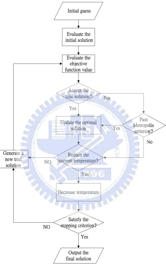
as the descent method. Figure 1 is the flowchart of the SA algorithm (Pham and

Karaboga, 2000). Yeh et al. (2007a) gave more detailed introduction on the

algorithm of SA. The SA been successfully applied to various types of problem such

as the THM forecast (Lin and Yeh, 2005), aquifer parameter estimation (e.g., Yeh and

Chen, 2007b; Huang and Yeh, 2007c), pipe wall surface reaction rate (Yeh et al.,

2008), and pumping source information (Lin and Yeh, 2008).

2.3 Tabu search

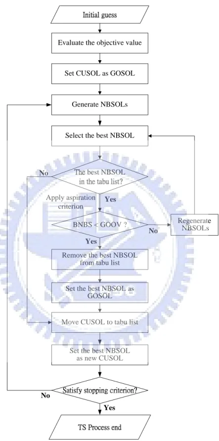
Glover (1986) proposed the two main concepts of TS: memory and learning.

The objective of tabu is through interdicted some attributes and improved the search

more efficient and accurate. Through memory and learning, the TS is able to have

more intensification and diversification in algorithm. Memory means to memorize

the passed by solutions and to avoid the repetition of evaluations. During the

process of learning, the prior result is memorized to influence the result of next

experiment. A better result may encourage the next trial to increase the accuracy of

the obtained solution. Then through the learning result, the following search can

focus on the better solutions but not wasting time on worse solutions. According to

encourage some trial solutions during the iterative process. The utility of the tabu

list is to memorize some lately evaluated trial solutions. The goal of the aspiration

criteria is to release some of the solutions memorized in the tabu list to avoid the

iteration cycling and may finally trap solutions in a local optimum. Figure 2

illustrates the flowchart of the TS algorithm. The TS been successfully applied to

identify optimal parameter structure (Zheng and Wang, 1996) and spatial pattern of

groundwater pumping rates (Tung and Chou, 2004).

2.4 Ordinal optimization

Recently, the OOA has been applied to many areas in terms of simulation-based

complex optimization problem. The OOA has two major tenets: ordinal comparison

and goal softening procedures. The ordinal comparison procedure is to see the

relative relationship between each solution because it is much easier to find better

solutions. The goal softening procedure is to determine a reliable and good enough

solution instead of directly evaluating the optimal solution in a complex optimization

model. The purpose of goal softening procedure is to reduce the consumption time

on computer calculation and to obtain the optimum solution from the feasible solution

space. To get the top proportion solutions is much easier than to find out the best

one. Lau and Ho (1997) showed that the OOA ensures that top 5% solutions can be

reliable.

According to the OOA, all the possible trials are estimated coarsely and ranked

quickly. The solution domain is divided to several different parts, the possible

optimum solution located in which sub-domain might be effortlessly to recognize.

The optimum solution can then be easily to obtain while all the calculation efforts are

focused in searching the possible sub-domain. Therefore, a crude model should first

be employed to estimate and rank the solution, and then the good solutions can be

differentiated from the bad solutions. Then, the goal softening procedure is focused

on the top proportion solutions to determine the optimum solution. Accordingly, the

simulation time can be reduced effectively. The OOA been successfully applied to

power system planning and operation (Guan et al., 2001; Lin et al., 2004), the

electricity network planning (Liu et al., 2006) and the wafer testing (Lin and Horng,

2006) and so on.

2.5 Roulette wheel

The roulette wheel selection method is an important part of GA. The key

concept of GA is survival of the fittest by natural selection. Better solutions have

good objective function values and thus the areas occupied on roulette wheel are

larger in proportion and their corresponding solutions will be selected with greater

constantly be selected. Strengthen and calculate in good solution nearby, will have a

very high chance to find out the global optimal solution. Through this method, much

time can be saved to avoid evaluating the bad solutions.

2.6 SATSO-GWT model

A new model called SATSO-GWT is developed based on SATS-GWT and OOA.

The objective function value in SATSO-GWT is to minimize the sum of square errors

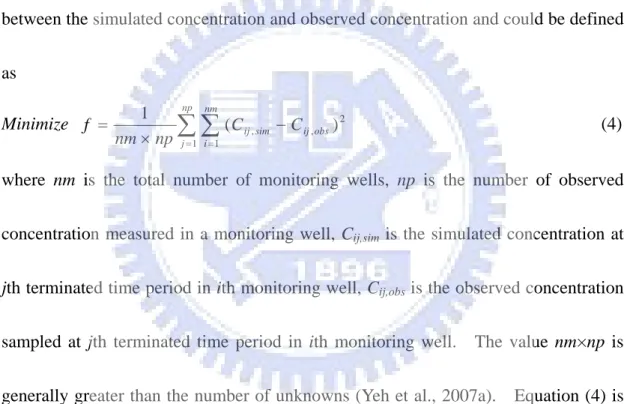
between the simulated concentration and observed concentration and could be defined

as Minimize 2 1 1 , , ) ( 1

_{∑ ∑}

= = − × = np j nm i obs ij sim ij C C np nm f (4)

where nm is the total number of monitoring wells, np is the number of observed

concentration measured in a monitoring well, Cij,sim is the simulated concentration at

jth terminated time period in ith monitoring well, Cij,obs is the observed concentration

sampled at jth terminated time period in ith monitoring well. The value nm×np is

generally greater than the number of unknowns (Yeh et al., 2007a). Equation (4) is

used to calculate the objective function value of the trial solution generated by the

approach.

Figure 3 shows the flowchart of SATSO-GWT while Figures 4 and 5 show the

flowchart of the TS process and OOA, respectively. TS and SA are used to generate

respectively. The objective function value is then calculated based on the sampled

concentrations and simulated concentrations generated based on those source location

and the release periods and concentrations. Each candidate location is regarded as

one sub-domain and the OOA is utilized to choose the best 5% sub-domains. The

best combination of the source location and the release periods and concentrations,

i.e., the least objective function value, is recorded at each sub-domain. Totally, NT

locations are generated by TS at each temperature; therefore, NT sets of best

combination are obtained. As the number of generated combinations reaches total

candidate locations about 3 times for several temperature levels, the top 5% best

sub-domains, can be sifted. After obtaining the top 5% best sub-domains, the

roulette wheel method is applied and the best combination regarding source release

information has more opportunity to be chosen when decreasing the temperature. In

reality, the real source location falls in the best combinations. The algorithm is

terminated when the objective function values are less than 10-6 four times

successively. Finally, the latest updated solution, including the estimated location

Chapter 3 Results and discussion

3.1 Example contamination site

An example groundwater contamination site is given to illustrate the source

information estimation procedure of the proposed algorithm SATSO-GWT. The

domain of the site is divided into 27X27X4 finite difference meshes in x-, y-, and z-

directions. The grid width and length are 20 m and the grid height is 6 m. Thus,

the total length and width of the site are both 540 m, and the aquifer thickness is 24 m.

Assume that the real source is located at S1 and consistently releases concentrations

of 100 ppm over the first 180 days and 50 ppm over the second 180 days. The

contaminant is assumed no decay and not adsorbed on the aquifer media. The site is

heterogeneous and divided into three different areas with the hydraulic conductivities

of being 20 m/day, 10 m/day, and 30 m/day in areas I, II, and III, respectively. The

aquifer porosity, specific storage, and hydraulic gradient are 0.3, 10-4 m-1, and 0.009,

respectively. The recharge rates are 120 mm/year, 80 mm/year, and 100 mm/year in

areas I, II, and III, respectively, in the first 180 days. The dispersion coefficients in

x-, y-, and z- direction are 40 m2/day, 10 m2/day, and 1 m2/day, respectively. The

finite difference grids are block-centered and the boundary conditions for the flow

system are shown in Figure 6. The slash grids represent the no flow boundary. The

located at (110 m, 270 m, -9 m) and releases a rate (Q) of 1 m3/day with the

concentrations of 100 ppm and 50 ppm over first and second 180 days. Yeh et al.

(2007a) mentioned that the number of sampling points should be greater than the

number of unknowns. There are at least seven unknowns to be determined in this

case study including the three coordinates of the source location and the two or more

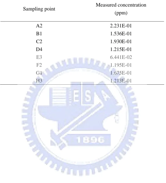
release periods and concentrations. Accordingly, eight sampling points, i.e., wells A

to H shown in Figure 6, with various depths are considered. Note that A2 means that

the sampling point is located at the second layer below the ground surface of the

monitoring well A. The measured concentrations at these sampling points are listed

in Table 1. The groundwater transport model MODFLOW-GWT developed by

(USGS) is utilized to generate the simulated concentrations at these monitoring wells

and the SATSO-GWT is used to identify the source information.

Before the source identification, a block with 3X3X4 meshes is delineated as a

suspicious area which contains the contamination source. Thus, there are 36

candidate sources within the block and one of the candidates is the target source.

The lower and upper bounds of the release period are taken as 0 day and 400 days,

respectively, and the release concentration are 0 ppm and 200 ppm, respectively. If

the release period and concentration should have accuracy to the first decimal place,

solution space is very huge and poses a large computational burden to find the target

source information. Therefore, the OOA is adopted in SATSO-GWT for the

identification. Once the generated combinations for the source location and the

source release periods and concentrations reach total candidate locations about 3

times, the top 5% combinations with different source locations could be sifted. To

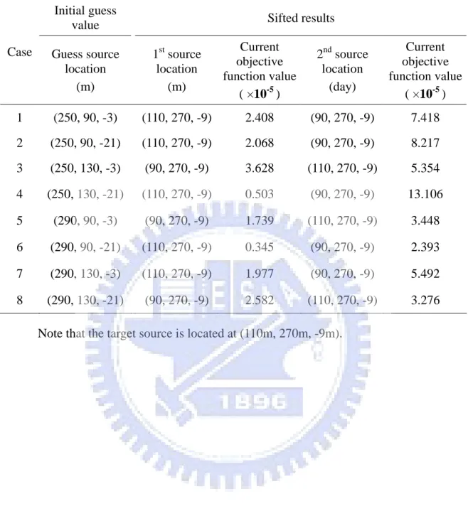
state more specifically, the top 2 best locations (36×0.05=1.8≈2) can be sifted.

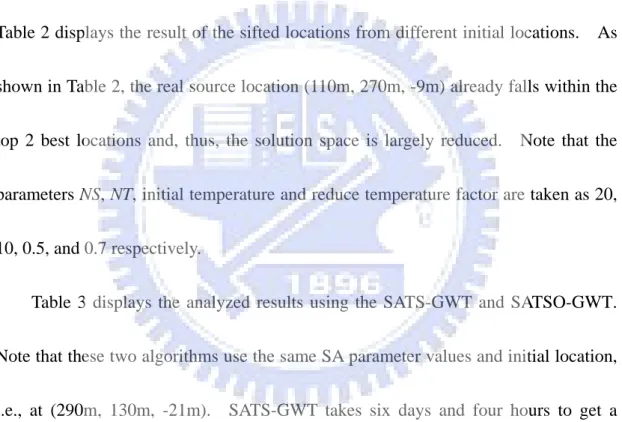
Table 2 displays the result of the sifted locations from different initial locations. As

shown in Table 2, the real source location (110m, 270m, -9m) already falls within the

top 2 best locations and, thus, the solution space is largely reduced. Note that the

parameters NS, NT, initial temperature and reduce temperature factor are taken as 20,

10, 0.5, and 0.7 respectively.

Table 3 displays the analyzed results using the SATS-GWT and SATSO-GWT.

Note that these two algorithms use the same SA parameter values and initial location,

i.e., at (290m, 130m, -21m). SATS-GWT takes six days and four hours to get a

fairly good result while SATSO-GWT only consumes one day and two hours and

obtain more accurate result on a personal computer with Intel Pentium D 3.2GHz

CPU and 1 GB RAM.

To examine the performance of SATSO-GWT, following three scenarios are

error, (3) the problem with a larger suspicious area with more complicated release

periods.

3.2 Effect of different initial location

The first scenario contains eight cases to study the effect of using different initial

location on the identify result. The target area of candidate location is rectangular.

Therefore, eight suspicious sources located right at the corners of the target area are

chosen to test the influence of the different initial location. Table 4 shows the

estimated results for the source location and two release periods and concentrations.

In these eight cases, the estimated source locations are all correct, i.e., the real source

location is located at (110 m, 270 m, -9 m). In addition, the estimated release

periods and concentrations in these eight cases are fairly good if compared with the

real release data.

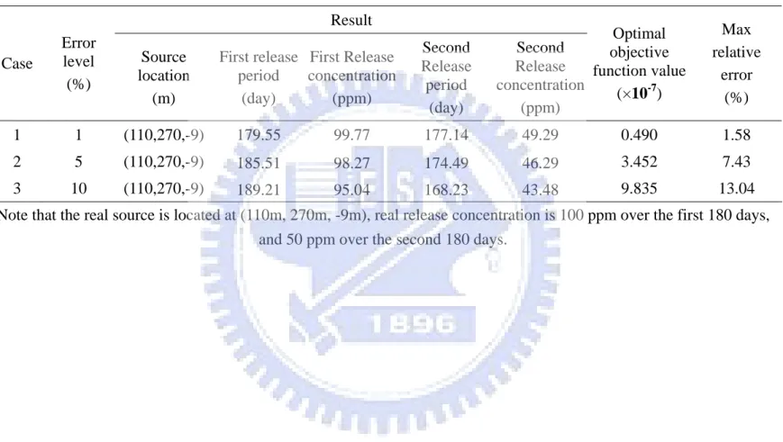
3.3 Effect of measurement errors

The second scenario is to test the performance of SATSO-GWT when the

simulated sampling concentrations contain random measurement errors. The

disturbed observed concentrations are expressed as (Mahar and Datta, 2001): ) 1 ( ₁ , ' , C Er RD C_iobs = _iobs× + × (5)

where is the disturbed observed concentration, Er is defined as the level of

measurement error, and RD1 is a random standard normal deviate generated by the

' ,obs

i

routine RNNOF of IMSL (2003). Three different values of Er, 1 %, 5 %, and 10 %,

are considered for this scenario.

The estimated results shown in Table 5 indicate that the source location is all

correctly identified when Er = 1 %, 5 %, and 10 %. When Er = 1 %, the max

relative error is only 1.58 % for the obtained two release concentrations and periods.

It shows that SATSO-GWT gives good estimated results when the measurement

errors are very small. As Er increased to 5 %, the max relative error in the obtained

results is 7.42 % occurred at the second release concentration. As Er = 10 %, the

estimated results show that the relative error for the first release period is 5.11 %, for

the first release concentration is 4.96 %, for the second release period is 6.54 %, and

for the second release concentration is 13.04 %. The max relative error occurs at the

second release concentration which deviates from the target concentration 6.5 ppm.

These results indicate that even the sampling concentrations contain measurement

error levels up to 10 %, the proposed SATSO-GWT still gives fairly good results.

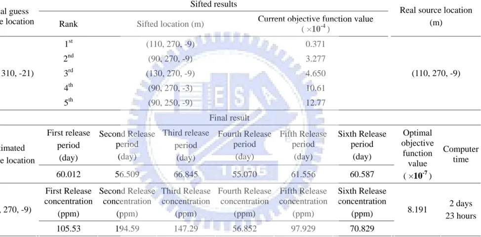
3.4 Larger suspicious area and more release periods

It has been shown that SATSO-GWT can reduce the problem domain based on

OOA for a complex combinatorial source information identification problem. Thus,

the last scenario is to test the ability of SATSO-GWT when applied to the case of a

layers) delineated by the broken lines as shown in Figure 7. On the source release

history, this scenario considers a more complicated release periods problem which has

the source release over one year and each two months is an interval. The release

history contains concentrations of 100 ppm, 200 ppm, 150 ppm, 50 ppm, 100 ppm,

and 70 ppm for those six intervals. Therefore, totally fifteen unknowns are

considered here, i.e., the location of three coordinates and six release periods with

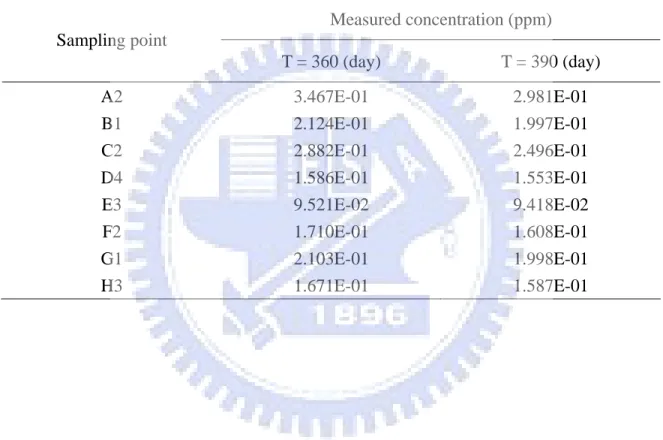
different concentrations. Accordingly, sixteen sampling data, i.e., wells A to H with

two different time period data are considered. Assume that the concentration data

are sampled twice, i.e., at the times 360 days and 390 days as listed in Table 6.

The parameter NT associated with the generated locations by TS at each

temperature is taken as 25 to accommodate larger candidate locations. Because the

number of the total candidate locations is 100, so the top 5 best locations are chosen

by the OOA. Table 7 displays the top 5 best locations and the estimated result of

SATSO-GWT. In Table 7, SATSO-GWT gives excellent results with the correct

source location and the estimated source release histories are very close to the target

one. In this scenario, the SATSO-GWT is utilized to simplify the problem domain

first, and then intensively searching the best fit solution from much smaller problem

domains. This scenario has fifteen unknown variables and the SATSO-GWT take

with Intel Pentium D 3.2GHz CPU and 1 GB RAM. Accordingly, even if the

suspicious areas is large and the release history is in a complicate pattern, the

SATSO-GWT demonstrates it ability in identifying the source information with good

Chapter 4 Concluding remarks

A new identification model SATSO-GWT has been developed based on the OOA

and SATS-GWT for solving the transient source release problem. The OOA is used

to find good solutions effectively for a problem with a large amount of unknowns.

The SATSO-GWT combines the merit of SA, TS, OOA, and roulette wheel method to

solve the complex source information identification problem effectively and

accurately. The SATSO-GWT utilized the spatial data to identify the source

information.

SATSO-GWT gives correct estimated location and good estimated release

periods and concentrations in eight cases with different initial guess location. In

addition, the SATSO-GWT gives fairly good results when the sampling concentration

having measurement errors, even the error level is up to 10%. For a large target area

with a complex release history which has six release periods with six different

concentrations, the SATSO-GWT can also give excellent results demonstrating its

capability in dealing with such the problem. According to the result of the final

scenario, the more complex release history problem could also be solved as long as

the computing time is long enough. The model SATSO-GWT provides effective

References

Aral, M. M., and J. Guan (1996), Genetic algorithms in search of groundwater

pollution sources, Advances in Groundwater Pollution Control and Remediation,

347-369.

Aral, M. M., J. B. Guan, and M. L. Maslia (2001), Identification of contaminant

source location and release history in aquifers, J. Hydrol. Eng., 6(3), 225-234.

Atmadja, J., and A. C. Bagtzoglou (2001), State of the art report on mathematical

methods for groundwater pollution source identification, Environmental

Forensics, 2(3), 205-214.

Bagtzoglou, A. C., D. E. Kougherty, and A. F. B. Tompson (1992), Applications of

particle methods to reliable identification of groundwater pollution sources,

Water Resour. Mgmt., 6(15-23).

Glover, F. (1986), Future path for integer programming and links to artificial

intelligence, Computers and Operation Research, 13(533-549).

Gorelick, S. M., B. Evans, and I. Remson (1983), Identifying Sources of Groundwater

Pollution - an Optimization Approach, Water Resour. Res., 19(3), 779-790.

Guan, X. H., Y. C. L. Ho, and F. Lai (2001), An ordinal optimization based bidding

strategy for electric power suppliers in the daily energy market, IEEE Trans.

Harbaugh, A. W., E. R. Banta, M. C. Hill, and M. G. McDonald (2000),

MODFLOW-2000, the U.S. Geological Survey Modular Ground-Water Model -

User Guide to Modularization Concepts and the Ground-Water Flow Process,

Open File Rep. 00-92, U.S. Geological Survey.

Ho, Y. C. (1999), An explanation of ordinal optimization: Soft computing for hard

problems, Inf. Sci., 113(3-4), 169-192.

Ho, Y. C., and M. E. Larson (1995), Ordinal Optimization Approach to Rare Event

Probability Problems, Discret. Event Dyn. Syst.-Theory Appl., 5(2-3), 281-301.

Ho, Y. C., R. S. Sreenivas, and P. Vakili (1992), Ordinal Optimization in DEDS,

Journal of Discrete Event Dynamic Systems, 2(61-68).

Huang, Y. C., and H. D. Yeh (2007), The use of sensitivity analysis in on-line aquifer

parameter estimation, J. Hydrol., 335(3-4), 406-418.

doi:10.1016/j.jhydrol.12.007.

Hwang, J. C., and R. M. Koerner (1983), Groundwater Pollution Source Identification

from Limited Monitoring Well Data .1. Theory and Feasibility, J. Hazard. Mater.,

8(2), 105-119.

IMSL (2003), Fortran Library User's Guide Stat/Library, Volume 2 of 2, Visual

Numerics, Inc., Houston, TX.

Method of Characteristics Solute-Transport Model (MOC3D), Water-Resources

Investigations Report 96-4267, U.S. Geological Survey.

Lau, T. W. E., and Y. C. Ho (1997), Universal alignment probabilities and subset

selection for ordinal optimization, J. Optim. Theory Appl., 93(3), 455-489.

Lin, S. Y., Y. C. Ho, and C. H. Lin (2004), An ordinal optimization theory-based

algorithm for solving the optimal power flow problem with discrete control

variables, IEEE Trans. Power Syst., 19(1), 276-286.

doi:10.1109/tpwrs.2003.818732.

Lin, S. Y., and S. C. Horng (2006), Application of an ordinal optimization algorithm

to the wafer testing process, IEEE Trans. Syst. Man Cybern. Paart A-Syst. Hum.,

36(6), 1229-1234. doi:10.1109/tsmca.2006.878965.

Lin, Y. C., and H. D. Yeh (2005), Trihalomethane species forecast using optimization

methods: Genetic algorithms and simulated annealing, J. Comput. Civil. Eng.,

19(3), 248-257. doi:10.1061/(asce)0887-3801(2005)19:3(248).

Lin, Y. C., and H. D. Yeh (2008), Identifying groundwater pumping source

information using optimization approach, Hydrological Processes,

22(3010-3019). doi:10.1002/hyp.6875.

Liu, C. X., and W. P. Ball (1999), Application of inverse methods to contaminant

Water Resour. Res., 35(7), 1975-1985.

Liu, Y., J. Chen, and M. Xie (2006), Distribution network planning based on the

ordinal optimization theory, Autom. Electr. Power Syst., 30(22), 21-24, 92.

Mahar, P. S., and B. Datta (1997), Optimal monitoring network and

ground-water-pollution source identification, J. Water Resour. Plan.

Manage.-ASCE, 123(4), 199-207.

Mahar, P. S., and B. Datta (2000), Identification of pollution sources in transient

groundwater systems, Water Resour. Manag., 14(3), 209-227.

Mahar, P. S., and B. Datta (2001), Optimal identification of ground-water pollution

sources and parameter estimation, J. Water Resour. Plan. Manage.-ASCE, 127(1),

20-29.

Mahinthakumar, G. K., and M. Sayeed (2005), Hybrid genetic algorithm - Local

search methods for solving groundwater source identification inverse problems, J.

Water Resour. Plan. Manage.-ASCE, 131(1), 45-57.

Milnes, E., and P. Perrochet (2007), Simultaneous identification of a single pollution

point-source location and contamination time under known flow field conditions,

Adv. Water Resour., 30(12), 2439-2446. doi:10.1016/j.advwatres.2007.05.013.

National Research Council (1990), Groundwater Models - Scientific and Regulatory

Neupauer, R. M., B. Borchers, and J. L. Wilson (2000), Comparison of inverse

methods for reconstructing the release history of a groundwater contamination

source, Water Resour. Res., 36(9), 2469-2475.

Neupauer, R. M., and J. L. Wilson (1999), Adjoint method for obtaining

backward-in-time location and travel time probabilities of a conservative

groundwater contaminant, Water Resour. Res., 35(11), 3389-3398.

Neupauer, R. M., and J. L. Wilson (2001), Adjoint-derived location and travel time

probabilities for a multidimensional groundwater system, Water Resour. Res.,

37(6), 1657-1668.

Pham, D. T., and D. Karaboga (2000), Intelligent Optimisation Techniques, Springer,

Great Britain.

Sciortino, A., T. C. Harmon, and W. W. G. Yeh (2000), Inverse modeling for locating

dense nonaqueous pools in groundwater under steady flow conditions, Water

Resour. Res., 36(7), 1723-1735.

Skaggs, T. H., and Z. J. Kabala (1994), Recovering the Release History of a

Groundwater Contaminant, Water Resour. Res., 30(1), 71-79.

Skaggs, T. H., and Z. J. Kabala (1995), Recovering the History of a Groundwater

Contaminant Plume - Method of Quasi-Reversibility, Water Resour. Res., 31(11),

Skaggs, T. H., and Z. J. Kabala (1998), Limitations in recovering the history of a

groundwater contaminant plume, J. Contam. Hydrol., 33(3-4), 347-359.

Snodgrass, M. F., and P. K. Kitanidis (1997), A geostatistical approach to contaminant

source identification, Water Resour. Res., 33(4), 537-546.

Sun, A. Y. (2007), A robust geostatistical approach to contaminant source

identification, Water Resour. Res., 43(2), 12. W02418.

doi:10.1029/2006wr005106.

Sun, A. Y., S. L. Painter, and G. W. Wittmeyer (2006a), A constrained robust least

squares approach for contaminant release history identification, Water Resour.

Res., 42(4), 13. W04414. doi:10.1029/2005wr004312.

Sun, A. Y., S. L. Painter, and G. W. Wittmeyer (2006b), A robust approach for iterative

contaminant source location and release history recovery, J. Contam. Hydrol.,

88(3-4), 181-196. doi:10.1016/j.jconhyd.2006.06.006.

Tung, C. P., and C. A. Chou (2004), Pattern classification using tabu search to identify

the spatial distribution of groundwater pumping, Hydrogeol. J., 12(5), 488-496.

doi:10.1007/s10040-004-0344-2.

Wagner, B. J. (1992), Simultaneous Parameter-Estimation and Contaminant Source

Characterization for Coupled Groundwater-Flow and Contaminant Transport

Woodbury, A., E. Sudicky, T. J. Ulrych, and R. Ludwig (1998), Three-dimensional

plume source reconstruction using minimum relative entropy inversion, J.

Contam. Hydrol., 32(1-2), 131-158.

Woodbury, A. D., and T. J. Ulrych (1996), Minimum relative entropy inversion:

Theory and application to recovering the release history of a groundwater

contaminant, Water Resour. Res., 32(9), 2671-2681.

Yeh, H. D., T. H. Chang, and Y. C. Lin (2007a), Groundwater contaminant source

identification by a hybrid heuristic approach, Water Resour. Res., 43(9), 16.

W09420. doi:10.1029/2005wr004731.

Yeh, H. D., and Y. J. Chen (2007b), Determination of skin and aquifer parameters for

a slug test with wellbore-skin effect, J. Hydrol., 342(3-4), 283-294.

doi:10.1016/j.jhydrol.2007.05.029.

Yeh, H. D., Y. C. Lin, and Y. C. Huang (2007c), Parameter identification for leaky

aquifers using global optimization methods, Hydrological Processes, 21(7),

862-872. doi:10.1002/hyp.6274.

Zheng, C., and P. Wang (1996), Parameter structure identification using tabu search

Table 1 The sampling points and measured concentrations when the real source is located at the depth of -9 m.

Sampling point Measured concentration

(ppm) A2 2.231E-01 B1 1.536E-01 C2 1.930E-01 D4 1.215E-01 E3 6.441E-02 F2 1.195E-01 G1 1.675E-01 H3 1.213E-01

Table 2 Results of 8 cases for sifting the top two locations Initial guess

value Sifted results

Case _{Guess source} location (m) 1st source location (m) Current objective function value ( ×10-5 ) 2nd source location (day) Current objective function value ( ×10-5 ) 1 (250, 90, -3) (110, 270, -9) 2.408 (90, 270, -9) 7.418 2 (250, 90, -21) (110, 270, -9) 2.068 (90, 270, -9) 8.217 3 (250, 130, -3) (90, 270, -9) 3.628 (110, 270, -9) 5.354 4 (250, 130, -21) (110, 270, -9) 0.503 (90, 270, -9) 13.106 5 (290, 90, -3) (90, 270, -9) 1.739 (110, 270, -9) 3.448 6 (290, 90, -21) (110, 270, -9) 0.345 (90, 270, -9) 2.393 7 (290, 130, -3) (110, 270, -9) 1.977 (90, 270, -9) 5.492 8 (290, 130, -21) (90, 270, -9) 2.582 (110, 270, -9) 3.276

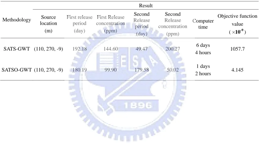
Table 3 Analyzed results from the SATS-GWT and SATSO-GWT Result Methodology Source location (m) First release period (day) First Release concentration (ppm) Second Release period (day) Second Release concentration (ppm) Computer time Objective function value ( ×10-9 ) SATS-GWT (110, 270, -9) 192.18 144.60 49.47 200.27 6 days 4 hours 1057.7 SATSO-GWT (110, 270, -9) 180.19 99.90 179.58 50.02 1 days 2 hours 4.145

Table 4 Results of 8 cases for studying the effect of different initial locations Initial guess

value Result

Case _{Guess source}

location (m) Source location (m) First release period (day) First Release concentration (ppm) Second Release period (day) Second Release concentration (ppm) Objective function value ( ×10-9 ) 1 (250, 90, -3) (110, 270, -9) 178.90 100.14 180.04 49.99 6.035 2 (250, 90, -21) (110, 270, -9) 180.25 99.65 179.41 49.92 6.053 3 (250, 130, -3) (110, 270, -9) 177.38 100.91 180.14 50.01 7.483 4 (250, 130, -21) (110, 270, -9) 179.86 99.99 180.11 49.97 2.031 5 (290, 90, -3) (110, 270, -9) 180.01 99.92 180.10 50.07 2.165 6 (290, 90, -21) (110, 270, -9) 180.14 99.80 179.55 49.91 4.520 7 (290, 130, -3) (110, 270, -9) 179.38 99.76 178.53 49.78 9.155 8 (290, 130, -21) (110, 270, -9) 180.19 99.90 179.58 50.02 4.145

Note that the real source is located at (110m, 270m, -9m), real release concentration is 100 ppm over the first 180 days, and 50 ppm over the second 180 days.

Table 5 Results of the cases when sampling concentrations have measurement error Result Case Error level (%) Source location (m) First release period (day) First Release concentration (ppm) Second Release period (day) Second Release concentration (ppm) Optimal objective function value (×10-7) Max relative error (%) 1 1 (110,270,-9) 179.55 99.77 177.14 49.29 0.490 1.58 2 5 (110,270,-9) 185.51 98.27 174.49 46.29 3.452 7.43 3 10 (110,270,-9) 189.21 95.04 168.23 43.48 9.835 13.04

Note that the real source is located at (110m, 270m, -9m), real release concentration is 100 ppm over the first 180 days, and 50 ppm over the second 180 days.

Table 6 The sampling points and measured concentrations when the real source is located at the depth of -9 m. Measured concentration (ppm) Sampling point T = 360 (day) T = 390 (day) A2 3.467E-01 2.981E-01 B1 2.124E-01 1.997E-01 C2 2.882E-01 2.496E-01 D4 1.586E-01 1.553E-01 E3 9.521E-02 9.418E-02 F2 1.710E-01 1.608E-01 G1 2.103E-01 1.998E-01 H3 1.671E-01 1.587E-01

Table 7 Results of the larger suspicious areas and more release periods Sifted results

Initial guess

source location _{Rank Sifted location (m)} Current objective function value

( ×10-4 )

Real source location (m) 1st (110, 270, -9) 0.371 2nd (90, 270, -9) 3.277 3rd (130, 270, -9) 4.650 4th (90, 270, -3) 10.61 (150, 310, -21) 5th (90, 250, -9) 12.77 (110, 270, -9) Final result First release period (day) Second Release period (day) Third release period (day) Fourth Release period (day) Fifth Release period (day) Sixth Release period (day) Estimated Source location 60.012 56.509 66.845 55.070 61.556 60.587 Optimal objective function value ( ×10-7 ) Computer time First Release concentration (ppm) Second Release concentration (ppm) Third Release concentration (ppm) Fourth Release concentration (ppm) Fifth Release concentration (ppm) Sixth Release concentration (ppm) (110, 270, -9) 105.53 194.59 147.29 56.852 97.929 70.829 8.191 2 days 23 hours

Note that the real source is located at (110m, 270m, -9m), real release concentration is 100 ppm over the first 60 days, 200 ppm over the second 60 days, 150 ppm over the third 60 days, 50 ppm over the fourth 60 days, 100 ppm over the fifth 60 days, and 70 ppm over the sixth 60 days.

No

Evaluate the objective value

Generate NBSOLs

Select the best NBSOL

best NBSOL

Yes

Yes No

Set the best NBSOL as new CUSOL Set CUSOL as GOSOL

Move CUSOL to tabu list

BNBS < GOOV ? Regenerate_NBSOLs

Remove the best NBSOL from tabu list

Set the best NBSOL as GOSOL Apply aspiration

criterion

Yes

No

Figure 2 Flowchart of TS algorithm. The CUSOL represents the current solution, GOSOL represents the global optimal solution, NBSOL represents the neighborhood solution, BNBS represents the best NBSOL, and GOOV represents the global optimal objective value.

3 times OFV

OFVCULO

Do TS process in SATSO-GWT (Figure 4)

Do OOA process in SATSO-GWT (Figure 5) Yes No Yes Yes No No

Figure 3 Flowchart of SATSO-GWT. The OFV represents the objective function value, CALO represents the candidate location, and OFVCULO represents the optimal objective function value at current location.

Figure 4 Flowchart of TS process in SATSO-GWT. The OFVGO represents the current global optimal objective function value, OFVCULO represents the optimal objective function value at current location, GOLO represents the global optimal location, CALO represents the candidate location, and CULO represents the current location.

Figure 5 Flowchart of OOA in SATSO-GWT. The CALO represents the candidate location.

S1 A D C B F G E H K = 20 m/day R = 120 mm/year K = 30 m/day R = 100 mm/year K = 10 m/day R = 80 mm/year No flow boundary No flow boundary Constant head and groundwater table is located at 0 m 20m 20m S1 540m 540m I II III

Figure 6 The groundwater flow system has an area of 540m by 540m and the problem domain is divided into three areas with different hydraulic conductivities and recharge rates. The real source is located at S1 and A to H represents the monitoring wells. The slash grids represent no flow boundary.

S1 A D C B F G E H K = 20 m/day R = 120 mm/year K = 30 m/day R = 100 mm/year K = 10 m/day R = 80 mm/year No flow boundary No flow boundary Constant head and groundwater table is located at 0 m 20m 20m S1 540m 540m I II III

Figure 7 A larger suspicious areas delineated by the broken lines with totally 100 suspicious areas (5 rows × 5 columns × 4 layers). The hydrogeological conditions of the flow system are the same as those shown in Figure 6.

個人資料

姓名：楊博傑 生日：民國73年3月29日 出生地：嘉義市 電話：03-3759611 住址：桃園市樹林八街9號6樓 學歷：民國95年畢業於國立中興大學環境工程學系 民國97年畢業於國立交通大學環境工程研究所