應用在太陽能光伏發電系統中的高效率全類比最大功率追蹤技術

國

立

交

通

大

_學

電控工程研究所

碩

士

論

文

應用在太陽能光伏發電系統中的高效率全類比

最大功率追蹤技術

Highly Efficient Analog Maximum Power Point

Tracking (AMPPT) in a Photovoltaic System

研究生：楊智宇

指導教授：陳科宏 博士

應用在太陽能光伏發電系統中的高效率全類比最大功率追

蹤技術

Highly Efficient Analog Maximum Power Point Tracking

(AMPPT) in a Photovoltaic System

研 究 生：楊智宇 Student：Chih-Yu Yang

指 導 教 授：陳科宏 Advisor：Dr. Ke-Horng Chen

國 立 交 通 大 學

電 控 工 程 研 究 所

碩 士 論 文

A Thesis

Submitted to Institute of Electrical Control Engineering

College of Electrical and Computer Engineering

National Chiao Tung University

in partial Fulfillment of the Requirements

for the Degree of

Master

in

Electrical Control Engineering

September 2011

Hsinchu, Taiwan, Republic of China

中華民國一百年九月

i

應用在太陽能光伏發電系統中的高效率全類比最大功率追

蹤技術

研究生：楊智宇 指導教授：陳科宏 博士

國立交通大學 電控工程研究所 碩士班

摘 要

本 論 文 利 用 類 比 電 路 的 設 計 ， 提 出 了 一 個 可 以 應 用 於 太 陽 能 光 伏 (Photovoltaic)發電系統中的最大功率追蹤技術(Maximum Power Point Tracking, MPPT)。論文一開始先探討了太陽能板的非線性特性。太陽能板鑒於不同的外在 溫度以及太陽光照度，因而存在著不同的最大功率點(Maximum Power Point,

MPP)。這些受外在環境影響的非線性特性嚴重地影響了太陽能板發電效率。論 文比較了現存的幾種最大功率追蹤技術之間的優劣，並提出了一個同時具有高追 蹤速度以及高追蹤效率的最大功率追蹤技術。太陽能發電系統的電壓電流操作範 圍受到外在環境因素的影響相當明顯，其操作範圍也因此相當大。因此在這篇論 文中，作者提出了一個具有大計算範圍的電流乘法器來滿足在最大功率追蹤上斜 率計算電路的需求。除此之外，太陽能板的最大功率點以及發電效能常受到周遭 建築物或是雲的遮蔽而改變。全域最大功率追蹤技術(Global Maximum Power

Point Tracking, GMPPT)可以進一步的實現在這篇論文所提出的最大功率追蹤技 術上，來提升整個太陽能發電系統的健全性與實用性。在論文的最後，相關的模 擬以及實驗結果證明了所提出的最大功率追蹤技術可達到追蹤效率 97.3%。除此 之外，所提出的太陽能發電系統並可將太陽能所產生的電力反饋回市電上，進而 拓展整個太陽能光伏發電系統的應用層面。

ii

Highly Efficient Analog Maximum Power Point Tracking

(AMPPT) in a Photovoltaic System

Student： Chih-Yu Yang Advisor： Dr. Ke-Horng Chen

Institute of Electrical Control Engineering

National Chiao-Tung University

ABSTRACT

A compact-size analog maximum power point tracking (AMPPT) technique is proposed in this thesis for high power efficiency in the photovoltaic (PV) system. Several MPPT techniques are studied at first to compare their pros and cons. The characteristics of solar array are introduced as well to address the difficulties when utilizing the solar energy. Combining the existing MPPT approaches, the thesis presents a fast and accurate tracking performance. The shading effect, which undermines the efficiency of solar array, is also discussed. The proposed MPPT technique can be further improved by global maximum power tracking (GMPPT) algorithm to guarantee its robustness. Here, a wide-range current multiplier, which tracks the maximum power point (MPP) in the solar power system, is implemented to detect the power slope condition of solar array. Simulation and experiment results show that the proposed MPPT technique can rapidly track the MPP with a high tracking efficiency of 97.3%. Furthermore, the proposed system can connect to the grid-connected inverter to supply AC power.

iii

誌 謝

在交大碩士班的生涯，轉眼間就快結束了。首先要感謝的是一路上提拔以及 支持我的指導教授 陳科宏老師。在研究方面，老師從碩一的一開始就給我了這 個頗具挑戰性的研究方向，因為是一個全新的研究主題，可以參考的文獻以及可 以請教的學長姐有限，老師總是我遇到問題時第一個會去請教的對象。一邊在老 師辦公室喝著老師親手煮的咖啡，一邊面對投影片上總總的問題，老師總是會指 引我一個方向，讓我自己去找答案，進而從解決問題的過程中，發掘到更多的新 知識。除此之外，也因為得到老師百分之百的支持，有機會利用碩二結束後的一 年時間，交換到德國慕尼黑工業大學一年，見識到了國外大學的上課風氣以及體 驗到了國外生活的種種經驗。 除此之外，還要感謝的是實驗室裡的學長姊、學弟妹們。昱輝學長除了總是 可以在我研究上遇到難題時，關鍵的給予建議，也時常一起在深夜的工五八樓窗 台旁，一起聊著過去大學時的懷舊時光，一起訴說著生活上面對到的難題，也一 起計劃著出國旅行的種種驚奇!俊禹、緯權、柄境、士榮、裕農、福貴學長們在 研究上的指導，玉萍、以萍、冠宇、淳仁、暐中等學弟妹們在生活樂趣上的分享。 另外還要感謝我最摯愛的爸媽以及熊小姐，爸媽總是無私的支持我的任何決 定，無論是在經濟上或是生活上，熊小姐則是一直能體諒我在研究上的辛苦，適 時的給我加油鼓勵，你們是我在台灣及國外生活時最大的精神支柱! 最後還要感謝的是大學以及研究所這幾年時間，無論是在國外或是台灣認識 的朋友、同學們，你們讓我的求學生涯豐富精采也值得回味! 楊智宇 國立交通大學 新竹 台灣 中華民國一百年九月

iv

Content

Content ... iv Figure Caption ... vi Table Caption ... ix Chapter 1 ... 1 Introduction ... 1

1.1 The Solar Energy and its Applications ... 1

1.2 Motivation ... 4

1.3 Thesis Organization ... 4

Chapter 2 ... 5

Maximum Power Point Tracking and the Proposed Solar System ... 5

2.1 The Characteristics of PV Module ... 5

2.2 MPPT Topology Studies ... 9

2.2.1 Perturbation and Observation (P&O) / Hill Climbing ... 9

2.2.2 Incremental Conductance ... 10

2.2.3 Fractional Open-Circuit Voltage ... 12

2.2.4 Fractional Short-Circuit Current ... 13

2.2.5 DC-Link Capacitor Droop Control ... 14

2.2.6 Load Current/Load Voltage Maximization ... 15

2.2.7 Pilot Cell ... 15

2.2.8 Model-Based Tracking... 16

2.2.9 Fuzzy Logic Control ... 16

2.2.10 Neural Network ... 17

2.3 The Proposed MPPT Solar System ... 20

Chapter 3 ... 21

The Proposed MPPT Algorithm ... 21

3.1 The Pros and Cons of Voltage-Based Tracking Algorithm ... 21

3.2 The Pros and Cons of Perturbation/Observation Tracking Algorithm 25 3.3 The Proposed Tracking Algorithm ... 28

v

3.4 Shading Effect and Global MPPT Algorithm ... 33

Chapter 4 ... 36

The Proposed Circuit of the MPPT Controller ... 36

4.1. Maximum Power Point Tracker Interface Topologies ... 36

4.1.1. The Basic Working Principles of Buck Converter ... 36

4.1.2. The Basic Working Principles of Boost Converter ... 40

4.1.3. Converter Topology Selection for MPP Tracker ... 44

4.2. Maximum Power Point Formula and Slope Calculation ... 45

4.3. Slope Detection Circuit ... 48

Chapter 5 ... 53

Simulation and Experiment Results ... 53

5.1 Simulation Results ... 53

5.1.1 PSIM Simulations ... 53

5.1.2 HSPICE Simulations ... 67

5.2 Experiment Results ... 78

Chapter 6 ... 86

Conclusion and Future Work ... 86

vi

Figure Caption

Fig. 2.1. Equivalent circuit of PV module. ... 8

Fig. 2.2. Characteristic curve of solar panel with respect to different irradiation levels. ... 8

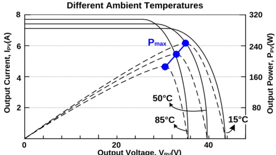
Fig. 2.3. Characteristic curve of solar panel with respect to different ambient temperatures. ... 8

Fig. 2.4. The flow chart of incremental conductance algorithm. ... 12

Fig. 2.5. Schematic of DC-link capacitor droop control MPPT. ... 14

Fig. 2.6. Structure of the neural network. ... 18

Fig. 2.7. The proposed grid-connected PV system. ... 20

Fig. 3.1. Photovoltaic current vs. photovoltaic voltage under different irradiation levels. ... 21

Fig. 3.2. Photovoltaic current vs. photovoltaic voltage under different ambient temperatures. ... 22

Fig. 3.3. The concept of voltage-based MPPT technique. ... 24

Fig. 3.4. The Perturbation and Observation Tracking Algorithm with Variable Perturbation Step Sizes. ... 27

Fig. 3.5. The concept of the proposed MPPT algorithm when irradiation reduces. .... 29

Fig. 3.6. The timing diagram of the proposed MPP tracking algorithm. ... 30

Fig. 3.7. The concept of the proposed MPPT algorithm when temperature reduces. .. 32

Fig. 3.8. The flowchart of the proposed MPP tracking algorithm. ... 33

Fig. 3.9. P-V Characteristic Curve due to non-uniform irradiation level. ... 34

Fig. 3.10. Flow chart of the global maximum power point tracking. ... 34

Fig. 3.11. P-V characteristic curve sketching the tracking of the global maximum power point due to non-uniform irradiation level. ... 35

Fig. 4.1 Schematic of a buck converter. ... 37

Fig. 4.2 The buck converter during phase 1. ... 37

Fig. 4.3 The buck converter during phase 2. ... 38

Fig. 4.4 The timing diagram of buck converter. ... 39

Fig. 4.5 Schematic of a boost converter. ... 41

vii

Fig. 4.7 The boost converter during phase 1. ... 41

Fig. 4.8 The timing diagram of boost converter. ... 43

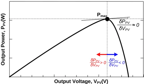
Fig. 4.9 The maximum power point on the power-voltage characteristic curve. ... 46

Fig. 4.10 The proposed slope detection circuit. ... 49

Fig. 4.11 The proposed wide-range squaring circuit. ... 52

Fig. 5.1 PSIM schematic of PV array with different solar irradiation levels... 54

Fig. 5.2 PV current vs. PV voltage with different irradiation levels. ... 55

Fig. 5.3 PV power vs. PV voltage with different irradiation levels. ... 55

Fig. 5.4 PSIM schematic of PV array with different temperatures. ... 56

Fig. 5.5 PV current vs. PV voltage with different temperatures. ... 56

Fig. 5.6 PV power vs. PV voltage with different temperatures. ... 57

Fig. 5.7 PSIM schematic for the solar array simulator. ... 57

Fig. 5.8 PSIM simulated PV characteristic curves. ... 58

Fig. 5.9 PSIM schematic of the proposed maximum power point tracker. ... 60

Fig. 5.10 Solar array simulator along with boost converter. ... 60

Fig. 5.11 PSIM schematic of the slope detection circuit. ... 61

Fig. 5.12 PSIM schematic of the perturbation circuit. ... 61

Fig. 5.13 PSIM schematic of OCT circuit. ... 62

Fig. 5.14 The output of solar array simulator at 30oC and 990 Watt/m2. ... 63

Fig. 5.15 The MPP tracking waveforms at 30oC and 990 Watt/m2. ... 64

Fig. 5.16 The MPP tracking waveforms at 30oC and 110 Watt/m2. ... 64

Fig. 5.17 The PSIM simulation waveforms under irradiation transition. ... 65

Fig. 5.18 The MPP tracking waveforms at 50oC and 990 Watt/m2. ... 66

Fig. 5.19 The MPP tracking waveforms at 5oC and 990 Watt/m2. ... 66

Fig. 5.20 The PSIM simulation waveforms under temperature transition. ... 67

Fig. 5.21 The HPSICE I-V simulation of the solar array. ... 68

Fig. 5.22 The simulated characteristic P-V curves according to different parameters. ... 70

Fig. 5.23 Simulation waveforms of duty cycle modulation.. ... 71

viii

Fig. 5.25 Duty cycle changes when the slope changes from negative to positive.. ... 74

Fig. 5.26 Simulation results of the proposed MPPT technique. ... 75

Fig. 5.27 Simulation results showing the effectiveness of the OCT technique.. ... 76

Fig. 5.28 Simulation results of the proposed MPPT technique undergoing environmental condition changes. ... 77

Fig. 5.29 Experiment prototype and chip micrograph. ... 78

Fig. 5.30 Tracking efficiency of the proposed MPPT algorithm and circuit. ... 80

Fig. 5.31 The waveforms of PV system during the system power-on period. ... 81

Fig. 5.32 The waveforms of VG according to different Eslope values. ... 82

Fig. 5.33 The waveforms of VPV, IPV and PPV during the power-on period.. ... 83

ix

Table Caption

TABLE 2.1 Efficiency Comparisons of Different PV Cells ... 5

TABLE 2.2 Summary of P&O and Hill Climbing Algorithm ... 10

TABLE 2.3 Slope Condition of the Operating Point ... 10

TABLE 2.4 Equations of Determining the MPP ... 11

TABLE 2.5 Comparisons between Different MPPT Techniques ... 19

TABLE 3.1 Comparisons between Voltage-Base Tracking and Perturbation and Observation Tracking... 28

TABLE 5.1 Slope Condition vs. Perturbation Direction ... 59

TABLE 5.2 Diode Factor vs. Maximum Power Point Voltage ... 69

TABLE 5.3 Technical Specifications of TYN-285P6 ... 79

1

Chapter 1

Introduction

1.1 The Solar Energy and its Applications

The global warming crisis has recently drawn worldwide public attention to issues related to energy conservation and alternative energy. Several energy conservation methods, such as energy recycling [1] and energy harvesting techniques [2], have been proposed to reduce unnecessary energy waste from commercial appliances. In addition, alternative energy, such as thermal [3], wind [4], or solar energy [5], is renewable and addresses pollution problems. Solar energy presents the advantages of low maintenance cost and pollution-free characteristics. These are keys to solving worsening global warming and reducing greenhouse gas emissions. Thus, this alternative energy has been gaining increasing popularity in numerous countries.

Solar energy may not be the most efficient choice with regard to energy production. Nevertheless, it still outweighs other kinds of energy, such as nuclear, coal, and gas energy, because it causes zero pollution, has no moving parts, and allows for easy maintenance. Despite these advantages, the overall energy production cost for solar energy is still too high compared with that incurred from gas or oil production. High costs restrict the wide-ranging global application of solar power systems. Generally, the low power efficiency of a solar power system is generally attributed to two factors. One is the conversion efficiency of the solar cell. The other is

2

related to the power efficiency of the system, or more specifically, the power efficiency on the power stage. The improvement of solar cell materials and relevant technology has continuously elevated the conversion efficiency of solar cells [6]. Conversion energy is reported to reach around 30% in today’s commercial products when a specific material is adopted [7].

Furthermore, enhancing the power efficiency of solar power systems enables the improvement of the efficiency of the power stage and the extraction of substantial energy from solar panels. The nonlinear physical characteristics of solar arrays, however, are inevitable obstacles to the highly efficient energy utilization of solar power systems.

The maximum available power supplied by a solar array depends on solar irradiation level and ambient temperature [8]. In practice, both these factors are difficult to precisely predict and measure. Thus, contemporary photovoltaic (PV) products, such as PV inverters [9] or solar chargers [10], are usually integrated with maximum power point tracking (MPPT) technique to extract the highest energy volume from solar arrays. Several MPPT algorithms exist [11]-[12]. Some of them are implemented using a microcontroller [13], field programmable gate array [14], and digital signal processors [15]. Others are implemented using analog or mixed signal methods [16]-[17]. For instance, in [18], a small-signal sinusoidal perturbation is injected into the switching frequency to compare the AC component. The average value of the solar array voltage is used to locate the maximum power point (MPP). In [19], the authors track the MPP by introducing a small-signal sinusoidal perturbation into the duty cycle of the switch and comparing the maximum variation in the input voltage and the

3

voltage stress on the switch. Ref. [20] uses the extremum-seeking control method to track the MPP. All of these tracking methods can exhibit high tracking efficiency. Unfortunately, they are implemented by discrete components instead of an integrated circuit (IC). In [21], a dual-module– based tracking technique, which compares the voltage and current difference between two solar arrays to track the MPP, is proposed. This method, however, increases hardware costs because each solar array has to be controlled by an individual tracker.

References [22] and [23] use the pilot cell to assist tracking. Nevertheless, the pilot cell should match the characteristics of the main solar array. In [24], a tracking solution is used to address the problems encountered during rapidly changing weather conditions. The technique incorporates an additional measurement of power in the middle of the MPPT sampling period. Furthermore, one can also use the information of the solar array, such as the diode quality factor and the reverse saturation current, to track the MPP [25]. Some methods combine two different tracking techniques to gain advantages. In [26] and [27], two tracking techniques are combined to improve tracking efficiency. The system switches between two tracking methods according to irradiation levels.

4

1.2 Motivation

Numbers of maximum power point tracking techniques exist in today’s commercial products and present in lots of literatures as mentioned before. However, most of the existing techniques are implemented by either the discrete components or the microcontrollers. In this proposed paper, a MPP tracker using single chip controller IC is proposed. The proposed MPP tracker features fast tracking speed and high tracking accuracy. In addition, the proposed system includes a boost DC-DC converter and a grid-connected PV inverter as well to convert the solar energy into the power grid for further use [28].

1.3 Thesis Organization

The thesis is organized as follows. In Chapter 2, the characteristics of the solar array are discussed in detail to show nonlinear behaviors and relevant cause factors. Some existing tracking algorithms are also discussed. Chapter 3 introduces the proposed MPPT algorithm used to extract the highest volume of energy from solar arrays. Circuit implementation is presented in Chapter 4 to demonstrate the proposed wide-range current multiplier used in the PV system intended for improving tracking efficiency. The simulation and measurement results, shown in Chapter 5, confirm the functionality and efficiency of the proposed MPPT system. Finally, Chapter 6 concludes the studies.

5

Chapter 2

Maximum Power Point Tracking and

the Proposed Solar System

2.1 The Characteristics of PV Module

PV cell or PV module is typically made of semiconductor materials, which is used to convert solar energy into electricity for further use. Based on different materials and different manufacture processes, there exists several PV cell types nowadays in the market and the conversion efficiency varies from each other. TABLE 2.1 summarizes the conversion efficiencies of different PV cell types. The conversion efficiency, however, is limited up to 30%. Considering the manufacture cost and the conversion efficiency, single crystalline silicon cell and multi-crystalline silicon cell are the two mostly used PV cells in today’s market.

TABLE 2.1 Efficiency Comparisons of Different PV Cells

Cell Material Cell Efficiency (%) Module Efficiency (%)

Single-Crystalline Silicon 22 10-15

Multi-Crystalline Silicon 18 9-12

Thin-Film Amorphous Silicon 13 10

Thin-Film Copper

IndiumDiselenide 19 12

Thin-Film Cadmium Telluride 16 9

High-Efficiency and

6

The characteristics of PV module vary with respect to different irradiation levels and different ambient temperatures. A simplified equivalent circuit [29] in Fig. 2.1 can facilitate the investigation of the nonlinear behaviors of PV module. The equivalent circuit consists of a current source, IL, which suggests the light-generated current; a diode, D1, which emulates the PN junction of a real PV cell; a series resistor, Rs, and a parallel resistor, Rp, which symbolize the parasitic series resistance and the parasitic parallel resistance on the PV module, respectively. The voltage generated at the terminals, VPV, is the voltage of the PV module, which can be multiplied through series-connected PV modules. Moreover, the current flowing out from the terminals, IPV, is the current of the PV module. The relationship between VPV and IPV can be shown in the following equations [30].





P s PV PV s PV PV os L PV R R I V R I V AkT q I I I         _     _   exp 1 (2.1) 3 1 1 exp _                    r r GO or os T T T T Bk qE I I (2.2)









100 25    S I K T I SC I L (2.3) where

IPV: PV module output current;

VPV: PV module output voltage;

Rp: parallel resistor;

Rs: series resistor;

Ios: PV module reversal saturation current;

A, B: ideality factors;

7

k: Boltzmann’s constant;

IL: light-generated current;

q: electronic charge;

KI: short-circuit current temperature coefficient at ISC;

S: solar irradiation (W/m²);

ISC: short-circuit current at 25°C and 1000 W/m²;

EGO: bandgap energy for silicon;

Tr: reference temperature;

Ior: saturation current at the temperature of Tr;

The equations verify that the characteristics of PV module depend on both temperature and solar irradiation. Fig. 2.2 and Fig. 2.3 show the IV curves sketched under different circumstances, which are different irradiation levels and different ambient temperatures. Under different irradiation levels, as shown in Fig. 2.2, the maximum power point (PMPP) increases as the solar irradiation increases, which means PMPP is proportional to the solar irradiation level. For different ambient temperatures, the IV curves act like Fig. 2.3. As can be seen in this figure,

PMPP decreases when the ambient temperature increases. That is to say,

PMPP is inverse proportional to the ambient temperature. These nonlinear

characteristics of PV module are crucial for analyzing and designing the PV system, especially for the maximum power point tracker.

8

Fig. 2.1. Equivalent circuit of PV module.

Fig. 2.2. Characteristic curve of solar panel with respect to different irradiation levels. IL Rp Rs

+

V

PV

-I

PV D1 O u tp u t P o w e r, P P V (W ) Output Voltage, VPV(V) O u tp u t C u rr e n t, IP V (A ) Pmax 8 6 4 2 80 160 240 320 40 20 0 1 kW/m2 0.75 kW/m2 0.5 kW/m2

Different Irradiation Levles

Fig. 2.3. Characteristic curve of solar panel with respect to different ambient temperatures. Pmax 8 6 4 2 80 160 240 320 40 20 0 50°C 85°C 15°C

Different Ambient Temperatures

O u tp u t P o w e r, PP V (W ) Output Voltage, VPV(V) O u tp u t C u rr e n t, IP V (A )

9

2.2 MPPT Topology Studies

There exist numerous maximum power point tracking algorithms in today’s market. This section discusses some of them and addresses their pros and cons.

2.2.1 Perturbation and Observation (P&O) / Hill Climbing

Perturbation and observation (P&O) method and hill climbing method are the two most common maximum power point tracking algorithms. P&O involves a perturbation in the operating voltage, and hill climbing, on the other hand, perturbs the duty ratio of the power converter connected to the PV modules. In the case of a PV module connected to a power converter, perturbing the duty ratio of power converter perturbs the PV module current and as a consequence perturbs the PV module voltage. Therefore, perturbation and observation method and hill climbing method are two tracking methods envisioning the same fundamental idea.

It can be seen in Fig. 2.2 and Fig. 2.3 that incrementing the voltage increases the power when the operating point is on the left side of the maximum power point (MPP) and decreases the power when the operating point is on the right side of the MPP. Therefore, if there is an increase in power, the subsequent perturbation should be remained the same to reach the MPP. Conversely, if there is a decrease in the power, the perturbation should be reversed to reach the MPP. TABLE 2.2 summarizes the ideas of perturbation and observation method and hill climbing method.

10

TABLE 2.2 Summary of P&O and Hill Climbing Algorithm

Perturbation Direction Change in Power Next Perturbation Direction

Positive Positive Positive

Positive Negative Negative

Negative Positive Negative

Negative Negative Positive

The process is repeated periodically until the MPP is reached. The system then oscillates around the MPP. The oscillation can be minimized by reducing the perturbation step size. However, a smaller perturbation step size slows down the tracing speed. There exist still other limitations that degrade the MPPT efficiency. For instance, as the amount of sunlight decreases, the Power-Voltage curve flattens out, as seen in Fig. 2.2. This makes it difficult for the MPPT to discern the location of the MPP, owing to the small change in power with respect to the perturbation of the voltage.

2.2.2 Incremental Conductance

The incremental conductance method is based on the fact that the slope of the PV module power curve is zero at the MPP, positive on the left of the MPP, and negative on the right, as summarized in TABLE 2.3.

TABLE 2.3 Slope Condition of the Operating Point

Position of the Operating Point Slope of the Power Curve

@ MPP 0 dV dP Left Side of MPP 0 dV dP Right Side of MPP 0 dV dP

11 Since

 

V I V I dV dI V I dV IV d dV dP        (2.4)

TABLE 2.3 can be reformulated into the following TABLE 2.4. The MPP

can, as a result, be tracked by comparing the instantaneous conductance (

V I

)

to the incremental conductance (

V I

 

).

TABLE 2.4 Equations of Determining the MPP

Position of the Operating Point Equation of Determining the MPP

@ MPP V I V I _   Left Side of MPP V I V I _   Right Side of MPP V I V I _  

Fig. 2.4 shows the flow chart of the incremental conductance tracking technique. Vop is the reference operating voltage at which the PV module is forced to operate. At the MPP, Vop is equal to VMPP, the maximum power point voltage. As long as the MPP is reached, the operation of the PV module is maintained at this point unless a change in ΔI is detected, which might indicate a change of the ambient temperature or a change of the sunlight irradiation level. If this scenario occurs, the tracking algorithm, judging the inequity equations, either increases or decreases Vop to track the new MPP. The increment size determines the tracking speed. Fast tracking can be achieved with larger incremental steps but the system might not operate exactly at the MPP, instead oscillates around it. As a result, there is a tradeoff between the tracking speed and the tracking accuracy.

12 Sense V(t), I(t) Calculate ΔV and ΔI ΔV = 0 ΔI = 0 ΔI/ΔV = -I/V

ΔI/ΔV > -I/V ΔI > 0

Increase Vop Decrease Vop Decrease Vop Increase Vop

Return Yes No Yes No Yes No No No Yes Yes

Fig. 2.4. The flow chart of incremental conductance algorithm.

2.2.3 Fractional Open-Circuit Voltage

The near linear relationship between the maximum power point voltage, VMPP, and the open-circuit voltage, VOC, of the solar array, under varying irradiation and temperature levels, has given rise to the fractional

VOC method.

OC V

MPP k V

V  (2.5)

where k is a constant of proportionality. Since V k is dependent on the V

characteristics of the solar array being used, it usually has to be computed beforehand by empirically determining VMPP and VOC for the specific solar array at different irradiance and temperature levels. The factor k has _V

13

Once the factor k is determined, V_V MPP can be computed by Eq. (2.5)

with VOC measured periodically by momentarily shutting down the power converter. Since Eq. (2.5) is only an approximation, the solar array technically never operates at the true MPP. Depending on the application of the PV system, this can sometimes be accurate enough for the system. Even if fractional VOC is not a true MPPT technique, it is very easy and cheap to implement as it does not necessarily require DSP or microcontroller control.

2.2.4 Fractional Short-Circuit Current

Fractional short-circuit current, ISC, results from the fact that, under varying atmospheric conditions, the maximum power point current, IMPP, is approximately linearly related to the ISC of the solar array.

SC I

MPP k I

I  (2.6)

where k is a proportionality constant. Just like in the fractional V_I OC technique, k has to be determined according to the solar array in use. The _I

constant k is generally between 0.78 and 0.92. _I

Using the fractional short-circuit current method to track the maximum power point seems to be easy to implement. However, measuring ISC during operation is problematic. One problem encountered is that an additional switch usually has to be added to the power converter to periodically short the solar array so that ISC can be measured using a current sensor. This increases the number of components and the hardware cost. Another problem is that the power output is not only reduced when detecting ISC but also because the MPP is never precisely matched as indicated by Eq. (2.6).

14

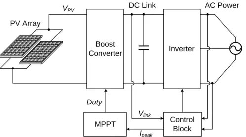
2.2.5 DC-Link Capacitor Droop Control

DC-link capacitor droop control is an MPPT technique that is specifically designed to work with a PV system that is connected in parallel with an AC system line as shown in Fig. 2.5.

The duty ratio of an ideal converter is given by

link PV

V V

Duty1 _(2.7)

where VPV is the voltage across the PV array and Vlink is the voltage across the DC link. If Vlink is kept constant, increasing the current going into the inverter increases the power coming out of the boost converter and in consequence increases the power coming out of the solar array. While the current is increasing, the voltage Vlink can be kept constant as long as the power required by the inverter does not exceed the maximum power available from the solar array. If that is not the case, Vlink starts drooping. Right before that point, the current control command Ipeak of the inverter is at its maximum and the solar array operates at the MPP. The AC system line current is fed back to prevent Vlink from drooping and Duty is optimized to bring Ipeak to its maximum, thus achieving MPPT.

Boost Converter Inverter MPPT Control Block DC Link Vlink Ipeak AC Power PV Array Duty VPV

15

2.2.6 Load Current/Load Voltage Maximization

The purpose of MPPT technique is to maximize the power coming out of the solar array. When the solar array is connected to a power converter, maximizing the solar array power maximizes the output power at the load of the converter as well. Conversely, maximizing the output power of the converter should maximize the solar array power, assuming a lossless converter is used.

Most loads can be of voltage-source type, current-source type, or resistive type. Therefore, for almost all loads of interest, it is adequate to maximize either the load current or the load voltage to maximize the load power. Nevertheless, operation exactly at the MPP is almost never achieved for the reason that this MPPT method is based on the assumption that the power converter is lossless.

2.2.7 Pilot Cell

In the pilot cell MPPT algorithm, the fractional voltage or current method is used, the point is that the open-circuit voltage or short-circuit current measurements are made on a small solar cell, called a pilot cell, which has the same characteristics as the cells in the larger solar arrays. The measurement results of the pilot cell can be used by the MPPT to operate the main solar array at its MPP, eliminating the loss of power during the VOC or ISC measurement. However, the fractional factor either

KV or KI is inconstant under varying environmental circumstances. As a

result, the tracking precision is greatly reduced. Furthermore, this method has a logistical drawback in that the solar cell parameters of the pilot cell

16

must carefully match to those of the main solar array. Thus, each pilot cell and solar array pair must be precisely calibrated, which increase the cost of the system.

2.2.8 Model-Based Tracking

If the values of the parameters in Eq. (2.1)~(2.3) are known for a given solar cell, the solar cell’s current and voltage could be calculated from measurements of the sunlight irradiation and temperature of the solar cell. The maximum power voltage could then be calculated directly, and the solar array operating voltage could be simply set equal to VMPP. Such algorithm is commonly called a model-based MPPT algorithm. Although appealing, model-based MPPT is usually not practical because the values of the cell parameters are not known with certainty, and in fact can vary significantly between cells from the same production run.

2.2.9 Fuzzy Logic Control

Microcontrollers have made using fuzzy logic control popular for MPPT over the last decade. Fuzzy logic controllers have the advantages of working with imprecise inputs, not needing an accurate mathematical model, and handling nonlinearity.

Fuzzy logic control generally consists of three stages: fuzzification, rule base table lookup, and defuzzification. During fuzzification, numerical input variables are converted into linguistic variables based on a membership function. The membership function is sometimes made less symmetric to give more importance to specific fuzzy levels.

17

The inputs to a MPPT fuzzy logic controller are usually an error E and a change in error ΔE. The user has the flexibility of choosing how to compute E and Δ E . Since dP/dV vanishes at the MPP, uses the approximation

 

  

_{  }



_

1 1      n V n V n P n P n E _(2.8) and

  

 1



 E E n E n (2.9)

Once E and ΔE are calculated and converted to the linguistic variables, the fuzzy logic controller output, which is typically a change in duty ratio ΔD of the power converter, can be looked up in a rule base table. The linguistic variables assigned to Δ D for the different combinations of E and ΔE are based on the power converter being used and also on the knowledge of the user.

In the defuzzification stage, the fuzzy logic controller output is converted from a linguistic variable to a numerical variable again using a membership function. This provides an analog signal that will control the power converter to the MPP.

MPPT fuzzy logic controllers have been shown to perform well under varying atmospheric conditions. However, their effectiveness depends a lot on the knowledge of the user or control engineer in choosing the right error computation and coming up with the rule base table.

2.2.10 Neural Network

Another MPPT algorithm well adapted for microcontrollers is by the method of neural network. Neural network commonly have three

18

layers: input, hidden, and output layers as shown in Fig. 2.6. The number of nodes in each layer varies and is user-dependent. The input variables can be solar array parameters such as VOC and ISC, atmospheric data like irradiation and temperature, or any combination of these. The output is usually one or several reference signals like a duty cycle signal used to drive the power converter to operate at the MPP.

How close the operating point gets to the MPP depends on the algorithms used by the hidden layer and how well the neural network has been trained. The links between the nodes are all weighted. The link between nodes i and j is labeled as having a weight of wij in Fig. 2.6. To accurately identify the MPP, the wij’s have to be carefully determined through a training process, whereby the solar array is tested over months or years and the patterns between the inputs and outputs of the neural network are recorded.

Since most solar arrays have different characteristics, a neural network has to be specifically trained for the solar array with which it will be used. The characteristics of a solar array also change with time, implying that the neural network has to be periodically retrained to guarantee an accurate MPPT.

i

j wij

Output Input Layer Hidden Layer Output Layer

Inputs

19

TABLE 2.5 summarizes a comparison between the mentioned maximum power point tracking algorithms based on the characteristics of solar array dependence, the genuineness of the MPP, the tracking speed and also the design and implementation complexity.

TABLE 2.5 Comparisons between Different MPPT Techniques

MPPT Technique PV Array Dependence True MPP Tracking Speed Design Complexity

Perturbation and Observation /

Hill-Climbing Independent Yes Varies High Incremental Conductance Independent Yes Varies High

Fractional Open-Circuit

Voltage Dependent No Fast Low

Fractional Short-Circuit

Current Dependent No Fast Low

DC-Link Capacitor Droop

Control Independent No Medium Low

Load Current / Load Voltage

Maximization Independent No Fast Low

Pilot Cell Independent No Varies High

Model-Based Tracking Dependent Yes Fast High

Fuzzy Logic Control Dependent Yes Fast High

20

2.3 The Proposed MPPT Solar System

In this thesis, an analog MPPT circuit with low-cost feature and high tracking efficiency is proposed. The proposed PV system is illustrated in Fig. 2.7. The proposed system includes a boost DC-DC converter, which serves the purpose of not only tracking the maximum power point of the solar arrays but also regulating the DC-link voltage, VBUS. The boost converter controller consists of a scaling circuit, an Open-Circuit Tracking (OCT) enable circuit, a sample/hold circuit, a slope detection circuit, a 7-bit up-down counter, and a PWM generator. Furthermore, the proposed PV system includes a grid-connected PV inverter as well to convert the solar energy to the power grid for further use. The full bridge inverter is controlled by a microcontroller. The islanding effect detection, in addition, is executed by the inverter controller as well to ensure the safety of the maintenance personnel.

IGBT1 IGBT2

IGBT3 IGBT4

Full Bridge Inverter

VT1 VT2 VT3 VT4 Grid L2 C2 RLoad Buffer Buffer VGrid VAC Solar Panels Scaling Circuit αVPV C1 MN L1

Full Bridge Inverter Controller

Boost Converter Controller with the Proposed MPPT Circuit

VT1 VT2 VT3 VT4 Track 0.7×Voc Slope Detection (dPPV/dVPV) S/H 7-bit Up-down Conuter PWM Generator OCT Enable Circuit CPV VPV IPV OCT Enable D βIPV Boost Converter D[0:7] ESlope VG Driver IAC VBUS VBUS

21

Chapter 3

The Proposed MPPT Algorithm

3.1 The Pros and Cons of Voltage-Based

Tracking Algorithm

As shown in Fig. 3.1 and Fig. 3.2, both the photovoltaic voltage and the photovoltaic current at the MPP can represent the MPP. For a particular operating condition, the control of MPPT normally regulates either the voltage or the current to a certain value that represents the local MPP. However, the mapping between MPP and these variables is time variant, as it is a function of changing irradiation and temperature. Ideally, however, this relationship is constant or changes slowly within a range. The photovoltaic voltage is a preferable control variable when it comes to the maximum power point tracking. The advantages of the voltage-based tracking are described in the following paragraph.

Photovoltaic Voltage, VPV(V) P h o to v o lt a ic C u rr e n t, IP V (A ) 8 6 4 2 40 20 0 1 kW/m2 0.75 kW/m2 0.5 kW/m2

Different Irradiation Levles

Large Variation

Small Variation

Fig. 3.1. Photovoltaic current vs. photovoltaic voltage under different irradiation levels.

22 8 6 4 2 40 20 0 50°C 85°C 15°C

Different Ambient Temperatures

Photovoltaic Voltage, VPV(V) P h o to v o lt a ic C u rr e n t, IP V (A )

Fig. 3.2. Photovoltaic current vs. photovoltaic voltage under different ambient temperatures.

Changing radiation causes the photovoltaic current to vary dramatically, as illustrated in Fig. 3.1. The fast dynamic of insolation is usually caused by the cover of mixed rapidly moving clouds. If the photovoltaic current is used as the set point, the MPPT requires a fast dynamic to follow a wide operating range from 0A to the short-circuit current because the current is heavily dependent on weather conditions. In contrast, the changing insolation only slightly affects the voltage of MPP. Fig. 3.2 shows that the cell temperature is the dominant factor varying the voltage of MPP when the temperature changes. However, cell temperature has a slow dynamic and is always within a certain range.

Unlike the current of MPP, the photovoltaic voltage of MPP is usually bounded to 70%~82% of the open-circuit voltage. This gives the tracking range a lower bound and an upper limit. When regulation of the photovoltaic voltage is implemented, the MPPT can quickly decide the initial point according to the percentage of the open-circuit voltage.

The photovoltaic current value at MPP is close to around 86% of the short-circuit current. Because the photovoltaic current dramatically varies

23

with insolation, the transient response of MPPT can occasionally cause the photovoltaic current to reach its saturation point, which is the short-circuit current. This shall be prevented because its nonlinearity causes a sudden voltage drop and results in power losses. However, for the regulation of photovoltaic voltage, the voltage saturations can be easily avoided because a controller knows the operating range is bounded around 70%~82% of the open-circuit voltage. Furthermore, a good-quality measurement of voltage signal is cheaper and easier than that of current measurement. Considering all the benefits of the voltage-based tracking aforementioned, as a result, the voltage-based tracking algorithm is preferred than the current-based tracking.

The voltage-based tracking technique, aside from the advantages of robustness and low solar irradiation dependence, holds also the advantage of fast tracking speed and low implementation complexity.

According to the relationship between the maximum power point voltage (VMPP) and the open-circuit voltage (VOC), the maximum power point tracker can take the advantage of this attribute to tack the MPP with high tracking speed. As illustrated in Fig. 3.3, the operating point can quickly jump to the point VMPP(approx) near the MPP if the open-circuit voltage is known. The tracker easily calculates the voltage of MPP from the information of open-circuit voltage. This can be achieved simply by dividing or multiplying the open-circuit voltage.

24 0 MPP VMPP(approx)

PV Voltage, V

PV

(V)

P

V

P

o

w

e

r,

P

P V

(W

)

MPP’ Irradiation Reduction Voc Voc’ 70%~82%

Fig. 3.3. The concept of voltage-based MPPT technique.

When the weather condition changes, say the irradiation reduces, the tracker has to disconnect the solar array and the power converter to create an open circuit on the system. This way, the new open-circuit voltage (VOC’), as indicated in Fig. 3.3, is detected. After getting the information of the new open-circuit voltage, the tracker can further calculate the new maximum power point (MPP’) and therefore regulate the operating point to be around this point. All in all, the voltage-based tracking algorithm benefits from its low design complexity, only a divider or a multiplier is needed to calculate the maximum power point. The fast tracking speed is also guaranteed in this technique, since there is no complicated calculation and iteration.

The voltage-based tracking algorithm, on the other hand, has some undesirable drawbacks as well. For example, the low power efficiency and the poor tracking accuracy.

The working principle of the voltage-based tracking technique is based on both the open-circuit voltage and the pre-determined percentage between maximum power point voltage and the open-circuit voltage. In order to constantly track the maximum power point, the open-circuit voltage of the

25

solar array needs to be updated periodically. Therefore, one has to disconnect the connection between the solar array and the power converter so that the real time open-circuit voltage can be recorded. In this way, the power delivery path between the solar array and the output stage is interrupted. It causes power loses as a result. Namely, the power delivery is discontinuous on the PV system and low power efficiency is presented, which is obviously undesirable for a PV system.

The second obstacle of the voltage-based tracking technique toward its perfection is the low tracking accuracy. As mentioned before in Chapter 2, the voltage-based tracking technique depends on the information of open-circuit voltage and the pre-determined or pre-measured coefficient kV. This coefficient, however, depends greatly on the manufacture material, the sunlight intensity, the environmental temperature and other factors. These factors are either time-varying or temperature-varying. As a result, it makes the determination and the measurement of the coefficient extremely difficult. Even though one can determine a desirable coefficient for a system, the environmental parameters, temperature, insolation, etc., vary along with the time, this makes the pre-determined coefficient inaccurate. Therefore, a high tracking accuracy cannot be guaranteed when the voltage-based tracking technique is used.

3.2 The Pros and Cons of Perturbation and

Observation Tracking Algorithm

The perturbation and observation tracking technique takes the advantage of calculating the slope of the power-voltage characteristic curve

26

to determine the maximum power point. Once the slope condition is determined, the perturbation direction can be consequently decided. It forces the system to operate toward the maximum power point. Based on this tracking idea, the tracking accuracy or the tracking effectiveness is guaranteed even under a varying environmental condition. The varying environmental condition changes the power-voltage characteristic curve and undoubtedly alters the maximum power point. To find out the new maximum power point, the perturbation and observation technique recalculates the slope of the new characteristic curve and determines the next perturbation direction. In this way, the changing atmospheric factors do not affect the tracking functionality. Instead, a high tracking accuracy can be further ensured with smaller perturbation steps.

The downsides of the perturbation and observation tracking technique, however, are the oscillation problem, low tracking speed, and the demanding design complexity.

Since the working principle of the perturbation and observation algorithm is to change the operating point step by step, the system can never operate exactly at the maximum power point. Instead, the operating point jumps back and forth around the actual maximum power point. This, therefore, causes an oscillation problem when the system reaches near the maximum power point. The power delivery loss and fluctuation, as a result, present on the PV system.

Before concluding the next perturbation direction, the controller has to deliberately calculate the slope of the characteristic curve at that time instant. This slows down the entire tracking process, compared to the voltage-based tracking algorithm. However, a faster tracking speed using

27

perturbation and observation method can still be achieved if the variable perturbation step method is used. As shown in Fig. 3.4, the size of perturbation step is not fixed. Variable step size is used to accelerate the tracking process. The farer the operating point away from the maximum power point, the larger the perturbation step size is. When the operating point is near the maximum power point, a smaller step size is used to guarantee an accurate tracking. Nevertheless, this may require a more complicated MPPT controller in the PV system.

Output Voltage, VPV(V) O u tp u t P o w e r, P P V (W ) Pmax

Variable Step Sizes

Fig. 3.4. The Perturbation and Observation Tracking Algorithm with Variable Perturbation Step Sizes.

The design complexity of the perturbation and observation tracking technique is higher than the voltage-based method. The MPPT controller needs to calculate the slope at any time instant, which means it requires a lot of arithmetic circuits and the circuits to determine the next perturbation direction. On the other side, the voltage-based tracking algorithm requires only a few circuits to find out the maximum power point from the open-circuit voltage.

28

To summarize, TABLE 3.1 gives the comparisons between the voltage-based tracking algorithm and the perturbation and observation tracking algorithm in terms of the tracking effectiveness, the tracking speed and the implementation complexity.

TABLE 3.1 Comparisons between Voltage-Base Tracking and Perturbation and Observation Tracking

Voltage-Based Tracking Perturbation and Observation Tracking

Tracking Accuracy Worse Better

Tracking Speed Faster Slower

Implementation Complexity Easier More complicated

3.3 The Proposed Tracking Algorithm

Fig. 3.5 demonstrates the concept of the proposed MPPT algorithm. Before the solar system turns on, the operating point of the PV system is located on the open-circuit voltage point, VOC. Conventional MPPT algorithm, such as slope detection algorithm [31] [e.g. perturbation/observation (P&O) algorithm or hill-climbing (HC) algorithm] calculates the slope of characteristic power-voltage curve to determine the slope condition and then to track the maximum power point (MPP). Nevertheless, as mentioned before, a PV system adopting this algorithm requires a lengthy amount of time to track the operating point from points

29 0 MPP Conventional Tracking Algorithm (1) OCT 0.7×Voc

Output Voltage, V

PV

(V)

O

u

tp

u

t

P

o

w

e

r,

P

P V

(W

)

(2) SDT (3) SDT MPP’ Irradiation reduces Voc

Fig. 3.5. The concept of the proposed MPPT algorithm when irradiation reduces.

Other tracking algorithms such as the constant voltage algorithm use a fixed ratio of maximum power voltage to open-circuit voltage VOC to approximate the MPP. Theoretically, 0.7 fractions of open-circuit voltage

VOC is close to the MPP [32]. Therefore, periodically disconnecting the

solar array and power stage to measure VOC and multiplying it to 0.7 can rapidly detect the current MPP, as described before. The fraction factor (0.7) varies when different solar cell materials are used. Moreover, it is considerably susceptible to environmental conditions such as ambient temperature and solar irradiation level. In this sense, the MPP cannot be guaranteed when varying environmental conditions are taken into consideration. Moreover, consistent disconnection between the solar array and power stage causes power delivery interruption during the sampling period, thereby resulting in the low power efficiency of the PV system.

To increase both tracking speed and accuracy while maintaining high power efficiency, the open-circuit tracking (OCT) algorithm and the slope detection tracking (SDT) algorithm are both adopted to track the MPP in this study. Disconnection between solar array and the power stage occurs

30

only one time; that is, in the beginning of the system power-on period. This way, unnecessary power loss can be avoided while maintaining the system power efficiency.

Fig. 3.6 illustrates the timing diagram of the proposed tracking algorithm. Eslope is a digital signal used to indicate the slope condition. Logic-high Eslope means the slope condition, dPPV/dVPV, of the solar panel is positive. On the contrary, logic-low Eslope means dPPV/dVPV is negative. The signal OCT Enable indicates whether the OCT tracking algorithm is enabled or not. The signal VG is the gate signal of the power NMOS in the boost converter. The signal IL1 shows the inductor current of the boost converter, which can also indicate the current of the solar panel.

VG T Dmax·T IL1 T D·T (D-∆D)T -∆D +∆D Time Time +∆D IL1(avg) -∆D +∆D

(1) Open Circuit Tracking Period (2) Slope Detection Tracking Period

Eslope Irradiation reduces Time OCT Enable Time

(3) Slope Detection Tracking Period

Fig. 3.6. The timing diagram of the proposed MPP tracking algorithm.

Basically, the tracking procedure can be divided into the following sequences.

31

The first step is: Before the solar system turns on, VOC is detected by the controller to set the PV panel voltage, VPV, close to 0.7×VOC for improving the tracking speed compared to the disadvantage of slow tracking speed in the conventional P&O and HC algorithms. Besides, the switching duty cycle of the boost converter is set to its maximum value in order to accelerate the tracking speed during the open-circuit voltage detection period.

The second step is: the SDT technique takes over the tracking procedure to continually and accurately track the MPP to make sure that the power stage receives the most energy from the solar panel.

The third step is: If the environmental condition changes, say, the irradiation level reduces, the slope condition changes from positive to negative, according to the solar cell characteristic shown in Fig. 3.1. Then,

Eslope transits from high to low. Aforementioned in Section 2.1, the voltage

is inversely proportional to the current. As a result, the SDT technique will increase the switching duty cycle. The current of solar array, therefore, increases to pull down the operating voltage and ensures the system operating move to a new maximum power point, MPP’, as illustrated in Fig. 3.5.

On the other hand, if the environmental temperature reduces, as shown in Fig. 3.7, the new maximum power point, MPP’, is higher than the old one, MPP. The PV system can still locate the new maximum power point through the proposed algorithm and then work on this new operating point.

32 0 MPP (1) OCT 0.7×Voc Output Voltage, VPV(V)

O

u

tp

u

t

P

o

w

e

r,

P

P V

(W

)

(2) SDT (3) SDT _MPP’ Voc Temperature reduces

Fig. 3.7. The concept of the proposed MPPT algorithm when temperature reduces.

The flowchart in Fig. 3.8 summarizes the overall tracking topology of the proposed MPP tracking algorithm. After the solar system turns on, the OCT technique is enabled until the operating voltage is set to be around 0.7×VOC. After that, the SDT technique consistently monitors the slope condition and makes sure the system operate at MPP regardless of any condition change in the environment. When the signal Eslope is set to be logic high, this may mean the irradiation level increases or the temperature reduces, the controller will decrease the switching duty cycle to the boost converter in order to pull down the inductor current. Meanwhile, the PV current is reduced as well and the PV voltage is increased conversely, which forces the system to operate toward the MPP. On the other hand, if the signal Eslope is detected to be logic low, the inductor current and the PV current is raised by the increased duty ratio. Therefore, the PV voltage is pulled down to track the MPP.

33

Fig. 3.8. The flowchart of the proposed MPP tracking algorithm.

The proposed AMPPT technique includes both the advantages of the OCT technique and the SDT technique. That is, the OCT technique can rapidly but roughly locate the MPP with fast tracking speed. In the meanwhile, the SDT technique improves the tracking accuracy which cannot be guaranteed by the OCT technique.

3.4 Shading

Effect

and

Global

MPPT

Algorithm

For a large scale photovoltaic system, unavoidable shadow from the nearby trees, cloud and buildings frequently cause the energy degradation of the solar array. The so called “partial shading effect” [33] poses a great threat to highly efficient utilization of the PV system. As depicted in Fig. 3.9, when the solar arrays are shaded, there exists more than one local

System Startup Eslope = 1 or 0 OCT SDT Duty ↓ Duty ↑ IPV ↓ & VPV ↑ PPV ↑ IPV ↑ & VPV ↓ PPV ↑ Moving toward MPP Moving toward MPP Eslope = 1 Eslope = 0 Reached 0.7×VOC ? Yes No

Slope Detection Tracking Period Open Circuit

34

maximum power point. As a result, the designed MPP tracker may easily misjudge the optimal operating point and therefore the system cannot provide its maximum energy. The proposed MPP tracking algorithm in this paper can be further improved by the algorithm provided in Fig. 3.10 to ensure the robustness of the PV system.

O u tp u t P o w e r, P P V (W ) Output Voltage, VPV(V) 0 Uniform Irradiation Non-Uniform Irradiation

Fig. 3.9. P-V Characteristic Curve due to non-uniform irradiation level.

Fig. 3.10. Flow chart of the global maximum power point tracking. LMPP Tracking

LMPP Reached?

Update Pmpp_last & Vmpp_last

Timer/Incidence triggered ? Yes No System Startup No GMPPT Start Vop’=Vop-ΔVperturb Vop=Vop’ Vop’=Vop+ΔVperturb Vop=Vop’ Ppresent > Pmpp_last ? Ppresent > Pmpp_last ? Yes Yes End GMPPT

Global Maximum Power Point Tracking

No

35

The system primarily determines whether it has reached its local maximum power point (LMPP). The measured power (Pmpp_last) and voltage (Vmpp_last) are then stored for later comparison. The control loop enters the global maximum power point tracking (GMPPT) stage when triggered by the timer. The default timer is set to 1 s. That is, the global maximum power point (GMPP) tracker is enabled every second to check whether the current operating point belongs to the GMPP. If the current operating point is already the maximum point on the power-voltage plane, the system will continuously operate at this point. Otherwise, the GMPP tracker locates the GMPP and forces the system to operate on the located point. During the GMPPT stage, the system is perturbed by a voltage difference ΔVperturb, which is approximated to 60%–70% of Voc [34], as sketched in Fig. 3.11. Thus, an MPPT technique guarantees full robustness of the connected PV system. O u tp u t P o w e r, P P V (W ) Output Voltage, VPV(V) 0 LMPP GMPP ΔVperturb MPP Tracking

Fig. 3.11. P-V characteristic curve sketching the tracking of the global maximum power point due to non-uniform irradiation level.

36

Chapter 4

The Proposed Circuit of the MPPT

Controller

4.1. Maximum Power Point Tracker Interface

Topologies

This chapter provides a comparative study with a goal of choosing the suitable converter topology for the application of maximum power point tracking in a PV system. Both the DC-DC buck converter and the DC-DC boost converter are usually used in the PV power system because of their simplicity and efficiency. The following paragraphs analyze both of these converter topologies and draw a conclusion of choosing the appropriate one for the maximum power point tracker in a PV system.

4.1.1. The Basic Working Principles of Buck Converter

Fig. 4.1 shows a schematic of a conventional DC-DC buck converter connected to a solar array. It comprises of a solar array as the power source, input and output capacitor, C1 and C2, respectively. A switch S and a diode

D are also presented in the figure. Rout is the summarized loading of the next stage, which is the DC-AC inverter in the proposed PV application.

Under the condition of continuous current mode, the operation of buck converter can be divided into two phases. In phase 1, as shown in Fig. 4.2, the switch S is turned on, which means it creates a short-circuit path