考慮電路延遲與障礙物迴避之直角史坦那樹建構法

國

立

交

通

大

學

資訊科學與工程研究所

碩

士

論

文

考慮電路延遲與障礙物迴避之

直角史坦那樹建構法

Performance-Driven Obstacle-Avoiding

Rectilinear Steiner Tree Construction

研 究 生：張書鑫

指導教授：李毅郎 博士

考慮電路延遲與障礙物迴避之直角史坦那樹

建構法

學生 : 張書鑫 指導教授：李毅郎 國立交通大學資訊科學與工程研究所

摘 要

隨著製程的演進，線路所造成的延遲已經變為最主要影響電路延遲的一個因 素。而且，在先進的積體電路設計中，對一些比較先進的設計進行繞線時，那些 設計常常會包含許多障礙物，例如: 區塊所產生障礙物，或者一些已經繞好的線 路。然而，避開障礙物的史坦那繞線研究卻很少考慮如何去減少電路延遲，大部 分之前的研究都只針對如何來減少整體繞線的長度，因此，這些研究被稱為避開 障礙物且最短繞線長度之直角史坦那樹 (OARSMT)。 這篇論文中，我們提出一個新穎且快速的演算法稱為關鍵樹幹為基礎之電路 延遲最小化演算法(critical-trunk based delay minimization algorithm)，在考慮障礙 物的情況下同時解決電路延遲問題。我們的演算法可以分為5個主要的部分; (1) 建立避開障礙物的擴張圖(spanning graph)，(2) 對遠離驅動源(driver)的接腳 (pin)先進行繞線，(3) 再連接其他的接腳(pin)，(4) 將歪斜的線轉化為水平或 垂的線段，(5) 優化違反時序限制最大的路徑延遲(Worst Negative Slack)。

實驗結果顯示，對於OARSMT，我們提出的演算法平均改進違反時序限制 最大路徑延遲和最大路徑延遲，分別是81.52 %以及28.42 %，而且，僅僅增加了 9.15%的線長，且外，我們更比[10]平均快了32.06%。對於C-Tree[21]，我們的 演算法相對改進的違反時序限制最大的路徑延遲和總線長，分別是53.92%以及 15.61%，我們提出的演算法更比[21]快了27.69倍。

Performance-Driven Obstacle-Avoiding Rectilinear Steiner Tree

Construction

Student：Shu-Hsin Chang Advisor：Yih-Lang Li Department of Computer Science

National Chiao Tung University

Abstract

With technology scaling, interconnect delay has dominated circuit delay. Mean-while, modern System on Chip (SOC) design contains many obstacles such as IP cores, macro blocks, and pre-routed nets within the routing region. Most previous works on obstacle-avoiding rectilinear Steiner tree construction only focus on mini-mizing total tree wire-length, and thus their works are called obstacle-avoiding recti-linear Steiner minimal tree (OARSMT).

In this thesis, we propose a novel and fast algorithm called critical-trunk based delay minimization algorithm to tackle timing issue regarding existing blockages. The proposed algorithm can be classified into 5 main steps: (1) construct an obsta-cle-avoiding spanning graph; (2) pre-route the sinks that are far away from the driver; (3) connect other sinks; (4) transform every slant edge into horizontal or vertical edges; (5) refine worst negative slack (WNS).

Experiments show that the proposed algorithm achieves the average reduction rates of WNS and maximum delay over OARSMT approach are 81.52 % and 28.42%. Besides, the proposed algorithm runs faster by 32.06% as compared to that in [10]. As compared to the C-Tree approach in [21], the reduction rates of WNS and wire length are 53.92% and 15.61%, respectively. The proposed algorithm achieves a 27.69X runtime speedup as compared to that in [21].

Acknowledgement

I am deeply grateful to my advisor, Doctor Yih-Lang Li for his continuous guid-ance, support, and ardent discussion throughout this research. His valuable sugges-tions help me to complete the thesis. I also express my sincere appreciation to all classmates in my laboratory for their help. Especially, I want to thank Jieyi Long and Professor Hai Zhou of Northwestern University for providing us with the test cases and binaries. I am grateful to all who have helped me.

Finally, this thesis is dedicated to my parents and my families for their patience, love, encouragement and long expectation.

Table of Contents

Abstract (Chinese) ... i

Abstract... ii

Acknowledgement... iii

Table of Contents ... iv

List of Figures... vi

List of Tables... ix

Chapter 1 Introduction...1

1.1 Preface...1

1.2 Obstacle-Avoiding Rectilinear Steiner Minimal Tree ...1

1.2.1 Maze Routing ...2

1.2.2 Spanning Graph Based Approaches...2

1.2.2.1 OASG Construction ...4

1.2.2.2 Tree Construction ...7

1.3 Performance-Driven Steiner Tree ...7

1.3.1 A-Tree Algorithm ...7

1.3.2 Prim and Dijkstra Algorithms ...9

1.3.3 Radius Ratio Based Approach ...10

1.4 Motivation...11

1.5 Contributions...12

1.6 Thesis Organization ...13

Chapter 2 Problem Formulation and Preliminaries ...14

2.1 Problem Formulation ...14

2.2.1 Elmore Delay Model...16

2.2.2 A* Search Algorithm...17

2.2.3 Region Tree (R-Tree) Algorithm...17

Chapter 3 PDOARST Algorithm...19

3.1 Steiner–Tree Delay Analysis...19

3.2 PDOARST Overflow ...23

3.3 OASG Construction ...26

3.4 SPT Construction ...29

3.4.1 Multi-Source Single-Target Maze Routing...30

3.4.2 A* Search Schemes ...31

3.5 Critical Trunk Growth...31

3.5.1 Critical Trunk Selection ...32

3.5.2 Rip-Up of Non-Critical Trunk ...32

3.6 Sub-Tree Re-Routing ...33

3.6.1 Delay Penalty Factor...33

3.6.2 Re-Routing Order and A* Search ...34

3.7 Transformation of Slant Edges into Rectilinear Edges...36

3.8 WNS Reduction ...37

Chapter 4 Extension to OARSMT Problem...40

Chapter 5 Experimental Results ...41

5.1 OARSMT Problem ...41

5.2 PD-OARST Problem ...42

Chapter 6 Conclusions...45

List of Figures

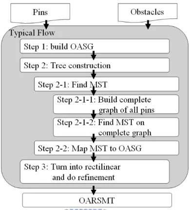
Figure 1- 1 : Flow chart of spanning graph based approach (typical flow of OARSMT) ...3 Figure 1- 2: An example of spanning graph approach. (a) Original

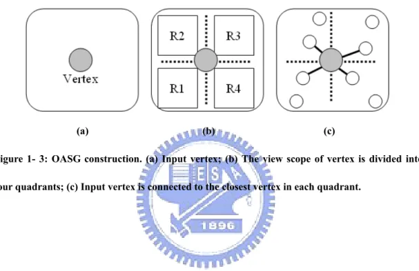
routing problem; (b) OASG construction; (c) the construction of the complete graph of all pins; (d) MST identification on the complete graph; (e) mapping of MST to OASG; (f) transformation of slant edges into horizontal and vertical edges...4 Figure 1- 3: OASG construction. (a) Input vertex; (b) The view scope of

vertex is divided into four quadrants; (c) Input vertex is connected to the closest vertex in each quadrant...5 Figure 1- 4: Pseudo-code of edge connection in Quadrant 1 (this

pseudo-code is quoted from [16])...6 Figure 1- 5: Comparison of normal Steiner tree and A-Tree ...9 Figure 1- 6: Steiner-tree topology changes as α varies between 0 and 1.

(a) Steiner tree is a SPT when α=1; (b) Steiner tree is a MST when

α=0; (c) Steiner tree contains the characteristics of SPT and MST

when α=0.5...10 Figure 1- 7: An example of the first heuristic method (H1). (a) The

routing problem of a driver and five sinks; (b) A RSMT is constructed; (c) The radius ratio for each sink is computed, and the radius ratios of the rightmost sink is too large (radius-ratio > α); (d) Rerouting the rightmost sink ...11 Figure 2- 1: (a) Obstacles are not allowed to overlap another obstacle;

(b) two obstacles can abut at one side or a corner...14 Figure 2- 2: Pins have to locate on the boundaries or at the corners of

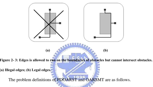
obstacles. (a) Illegal pin locations; (b) legal pin locations. ...15 Figure 2- 3: Edges is allowed to run on the boundaries of obstacles but

cannot intersect obstacles. (a) Illegal edges; (b) Legal edges. ...15 Figure 2- 4: An example of Elmore delay computation...16 Figure 2- 5: An example of Region Tree (R-Tree). (a) Rectangle A, B, C,

D, E are the inputted spatial data, and R1, R2 are minimum bounding rectangles generated by R-Tree; (b) How R-Tree to store these spatial data...18

Figure 3- 1: Relation between radius and delay in SPT. The bolded rectangle nodes on left-upper side of two figures are the drivers. The circled and bold nodes on right-lower side of the left figure are the sinks whose radiuses are longer than 80% of the worst radius in SPT. The circled and bold nodes on right-lower side of the right figure are the sinks whose delays are larger than 95% of the worst

delay in SPT. ...20

Figure 3- 2: Relation between radius and delay in MST. The bolded rectangle nodes on left-upper side of two figures are the drivers. The circled and bold nodes on right-lower side of the left figure are the sinks whose radiuses are longer than 80% of the worst radius in MST. The circled and bold nodes on right-lower side of the right figure are the sinks whose delays are larger than 95% of the worst delay in MST...20

Figure 3- 3: The topology of the proposed timing-driven Steiner tree..21

Figure 3- 4: An example of the critical-trunk growth (gray and bold lines) under the situation of criticality threshold factor to be 0.854. The bold node on upper side is the driver...22

Figure 3- 5: An example of critical-trunk growth (gray and bold lines) under the situation of criticality threshold factor to be 0.473. The bold node on right-lower side is driver...23

Figure 3- 6: Overall flow of critical-trunk based delay minimization algorithm...24

Figure 3- 7: The result of every step of the proposed critical-trunk based delay minimization algorithm. (a) Input problem. The bold and bigger node at the right bottom corner is the driver and other nodes are the sinks; (b) Construct OASG; (c) Grow critical trunks; (d) Sink routing; (e) Transformation of slant edges into horizontal and vertical edges...26

Figure 3- 8: Overall flow of OASG construction...26

Figure 3- 9: Step 2: Edge connection in Quadrant 1...27

Figure 3- 10: Step 3: Edge connection in Quadrant 2...28

Figure 3- 11: Step 4: Edge connection in Quadrant 3...28

Figure 3- 12: Step 5: Edge connection of Quadrant 4...28

Figure 3- 13: An example result of OASG construction...29

Figure 3- 14: An example of identifying new sources. (a) The two-pin net to be routed; (b) Bounding box and expanded bounding box for searching new sources; (c) One new source is identified...31

Figure 3- 15: An example of performing multi-source single-target maze routing with the cost function of SPT-driven A* search. The bold node on upper side is the driver...31 Figure 3- 16: The result of specifying critical trunks in the SPT. The

bold node on upper side is the driver. The gray and bold lines are critical trunks. The circled and bold nodes are critical sinks. ...32 Figure 3- 17: The result of ripping up the paths not on critical paths.

The bold node is the driver...33 Figure 3- 18: The example of determining delay-penalty-factor

calculation...34 Figure 3- 19: DPF inheritance makes sure that subsequent re-routings

will follow Rule 1 to complete sub-tree re-routing. (a) The DPFs of nodes a, b and c initially are zero; (b) The DPFs of nodes a and b set to be 0.6 and 0.2, respectively, by DPF inheritance; (c)

Subsequent re-routing connects nodes b and c instead of a and c to achieve a better delay at critical sink. ...36 Figure 3- 20: An example of transformation of slant edges into

rectilinear edges...36 Figure 3- 21: Two examples of redundant edge removal...37 Figure 3- 22: The flow of redirect mechanism to reduce worst negative

slack...38 Figure 3- 23: An example of one round of redirect mechanism (a) find

WNS sink (b) disconnect WNS sink in tree (c) find the best node to connect WNS sink on OASG (d) turn slant edge into rectilinear. .39 Figure 4- 1: Modified PDOARST algorithm for OARSMT problem ...40

List of Tables

Table 5- 1: The comparisons of tree wire-length and execution run-time among [9], [10], [16] and our OARSMT approach ...42 Table 5- 2: The Comparison of WL (wire-length), WD (worst delay of

circuit), WNS (worst negative slack of circuit) and execution run-time between our OARSMT and our critical-trunk based delay minimization algorithm...43 Table 5- 3: The Comparison of WL (wire-length), WNS (worst negative

slack of circuit) and execution run-time between C-Tree and our critical-trunk based delay minimization algorithm. ...44

Chapter 1 Introduction

1.1 Preface

Routing stage plays a crucial role in the physical design of VLSI integrated cir-cuits. The Steiner tree construction, as an extremely important step for routing, sig-nificantly affects the routing result. Furthermore, with dramatic increase in the com-plexity of VLSI circuits and decrease in the feature size of VLSI technology, inter-connect delay has dominated circuit performance in nanometer designs. Therefore, the problem of constructing a rectilinear Steiner tree (RST) with minimum delay has been widely studied.

With the trend toward IP-block-based System-on-Chip (SOC) design, IP cores, logic blocks and pre-routed wires are placed in the core before routing and then are regarded as blockages, which may significantly lengthen wires and induce delay dete-rioration. Consequently, it is desired to design a good performance-driven Steiner tree algorithm under obstacle-avoiding constraint. In this thesis, we present a very effi-cient algorithm to solve the rectilinear routing tree construction problem with simul-taneously considering timing delay and obstacles.

1.2 Obstacle-Avoiding Rectilinear Steiner Minimal Tree

Given a set of pins and a set of obstacles on a plane, an obstacle-avoiding recti-linear Steiner minimal tree (OARSMT) problem is to construct a Steiner tree of minimal total wire length such that all pins are connected using vertical and horizontal edges without intersecting any obstacle. The OARSMT problem has received in-creasing attentions in recent works, such as [9], [10] and [16]. The algorithms adopted in previous researches can be briefly classified into two major categories: (1) maze

routing and (2) spanning graph based approach.

1.2.1 Maze Routing

Traditional maze routing algorithm [31] and its following works, such as [30] and [32], can finds an optimal or near optimal path from source to target by wave propagation. However, it requires large execution time and memory usage for modern SOC designs. As a result, maze routing based approach becomes less popular for modern applications.

1.2.2 Spanning Graph Based Approaches

The connection graph is first constructed by the pins and four corners of each obstacle. The connection graph is named as an obstacle-avoiding spanning graph (OASG). The OASG guarantees to contain at least one desired solution in the graph. Besides, this approach has a more global view in terms of pins as well as obstacles and a good non-intersection property between the spanning edges and obstacles. Due to theses advantages of OASG, most previous works on the OARSMT problem, such as [9], [10] and [16], utilized the OASG to eliminate the impact of obstacles during Steiner tree construction. Secondly, they tried to find the desired solution from the spanning graph. Finally, they turned the slant edges into horizontal and vertical lines. Figure 1.1 displays the overall flow as follows:

Figure 1- 1 : Flow chart of spanning graph based approach (typical flow of OARSMT)

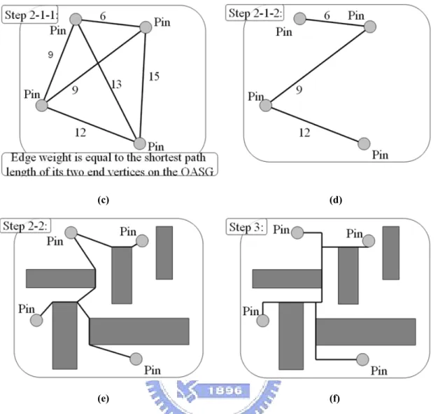
Figure 1.2 displays an example for explaining the operation flow of OARSMT. Notice that, in step 2-1-1 in Fig. 1-1, the weight of an edge on the complete graph is equal to the shortest path length of its two end vertices on the OASG.

(c) (d)

(e) (f)

Figure 1- 2: An example of spanning graph approach. (a) Original routing problem; (b) OASG

construction; (c) the construction of the complete graph of all pins; (d) MST identification on the

complete graph; (e) mapping of MST to OASG; (f) transformation of slant edges into horizontal

and vertical edges.

After having an overall understanding of spanning graph based approach, in the following sections, we shortly discuss the step 1 (OASG construction) and step 2 (Tree Construction).

1.2.2.1 OASG Construction

The OASG in [9] and [16] is constructed by first dividing the view scope of each vertex (pin or corner of each obstacle) into four quadrants, and then performing sweep

line algorithm to connect the closest one vertex in each quadrant. Figure 1-3 displays an example of OASG construction adopted in [16]. The view scope of the vertex un-der processed is divided into four quadrants, and then the vertex connects to the clos-est vertex in each quadrant using the algorithm described in Fig. 1-4 by the edge con-nection in Quadrant 1. The operations in the remaining quadrants can be easily de-duced by symmetric and mirroring mappings.

(a) (b) (c)

Figure 1- 3: OASG construction. (a) Input vertex; (b) The view scope of vertex is divided into

Figure 1- 4: Pseudo-code of edge connection in Quadrant 1 (this pseudo-code is quoted from [16])

We maintain two sets. The first set is an active vertex set called Av. It contains the vertices whose closest neighbors in Quadrant 1 are still not found. The second sets are two active edge sets called Aev and Aeh. These two edge sets are used to contain border of rectangular obstacle. Aev is for storing vertical edge and Aeh is for storing horizontal edge. Therefore, we can query these two edge set to check whether inter-secting obstacles.

After introducing the used data structure in algorithm, we briefly describe how to do edge connection. First, all the vertices presenting both pins and corners of obsta-cles are sorted by (x + y) in an increasing order, and then the sweeping algorithm is performed to process the sorted vertices. The currently scanned vertex v is connected to a vertex u in Av that has v in its Quadrant 1 if the Manhattan path between v and u

does not intersect any rectangular obstacle. Second, the vertex u is removed from Av since vertex u has already found its closet neighbor.

1.2.2.2 Tree Construction

Traditional OARSMT algorithms start to seek a tree on the OASG after OASG construction. The process of tree construction can be briefly divided into two main steps. The first step is finding a MST on the complete graph which is constructed by presenting every pin by a unique vertex and setting the weight of every edge using the shortest path length of its two end vertices on the OASG. Then, the shortest path length for every pin pairs is computed by Dijkstra or Floyd-Washall algorithm. Sub-sequently, either Kruskal or Prim algorithm is employed to obtain the minimum span-ning tree on the complete graph. The second step is mapping MST back to the OASG.

1.3 Performance-Driven Steiner Tree

As compared to timing-driven Steiner tree problem, OARSMT problem attempts to minimize total wire-length. However, it might worsen the performance if the criti-cal-path length is lengthened to increase the delay of critical sink. Performance-driven Steiner tree problem has to reduce the critical-path length to meet timing constrains, also with minimum total wire-length. The followings are some previous works on performance-driven Steiner tree problem.

1.3.1 A-Tree Algorithm

A-Tree algorithm [4] first analyzes the delay of distributed RC circuit as follows. Given a distributed RC circuit, the signal delay upper bound is computed by

Delay upper bound =

∑

× (1)

k node all k k C R _ _ * *

, where Rk*is the resistance between the driver and the node k, and Ck* is capacitance

at the node k. Assume that a unit-grid-length wire has wire resistance Ro and wire

ca-pacitance Co. Therefore, Formula (1) can be rewritten as follows:

Delay upper bound =

∑

(2)

∈ + × × + T k k o k o d R P T C C R | ( )|) ( ) ( =

∑

+ ∈ × T k o d C R

∑

∈ × × T k k k o P T C R | ( )| + (3)

∑

∈ × × T k o k o P T C R | ( )| +

∑

∈ × T k k d C R

, where Rd is the driver resistance, Pk(T) is the path from the source to node k in the

routing tree T, |Pk(T)| is the length of the path Pk(T), and Ck is the extra capacitance

besides the wire capacitance at node k in T if node k is a sink. Finally, Formula (3) is rewritten as follows in [4]:

Delay upper bound = t1(T) + t2(T) + t3(T) + t4(T) (4)

, where t1(T) = R_d ×C_o×length(T) t2(T) = ×

∑

× k ks all k k o P T C R _ sin _ | ) ( | t3(T) =

∑

∈ × × T k k o o C P T R | ( )| t4(T) = ×

∑

k ks all k d C R _ sin _

The definitions of t1(T), t2(T), t3(T) and t4(T)) are stated as follows.

(1) tl(T): tl(T) is the product of the driver’s output resistance and the total wire ca-pacitance. tl(T) is minimized when length(T) is minimum. In short, minimizing

tl(T) results in an optimal Steiner tree (OST).

(2) t2(T): t2(T) is a product of the path-length |Pk(T)| from the driver to the sink k in T

and the loading capacitance ck of each sink. t2(T) is minimized when all paths from the driver to sinks are minimum in length, which results in a shortest path tree (SPT) rooted at the driver. Therefore, minimizing t2(T) leads to a SPT.

(3) t3(T): t3(T) is proportional to the summation of the path length from the source to all nodes (not only sinks) in T. If there is a long driver-to-sink path in T, t3(T) will be very large since it contains a term which is substantially proportional to the square of path length |Pk(T)|. Hence, a routing tree of short paths is preferable in

[4] to keep t3(T) small. On the contrary, if length(T) and the number of nodes in T is large, it may increase t3(T) as well. Therefore, minimizing t3(T) tends to yield a routing tree between a SPT and an OST. A quadratic minimum Steiner tree (QMST) is referred to as a optimal tree under t3(T) in [4].

(4) t4(T): t4(T) is a constant.

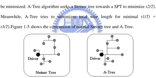
In order to minimize delay upper bound, the value of t1(T) + t2(T) + t3(T) should be minimized. A-Tree algorithm seeks a Steiner tree towards a SPT to minimize t2(T). Meanwhile, A-Tree tries to minimizes total wire length for minimal t1(T) +

t3(T).Figure 1-5 shows the comparison of normal Steiner tree and A-Tree.

Figure 1- 5: Comparison of normal Steiner tree and A-Tree

1.3.2 Prim and Dijkstra Algorithms

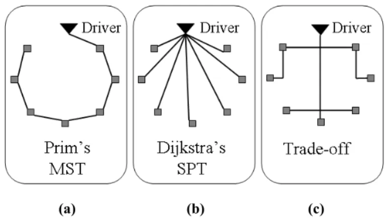
Timing delay analysis in distributed RC tree structures shows the influence of tree cost (total wire-length) and tree radius (path length from driver to sink) on signal delay of VLSI interconnects. A new and efficient interconnection tree construction is proposed in [5] to smoothly combine the objectives of minimum cost and minimum radius using Prim and Dijkstra algorithms, respectively. The topology of Steiner tree

is determined by a user-specified parameter α, ranging between 0 and 1. The obtained Steiner tree will be a SPT as α is equal to 1. If α is equal to 0, the Steiner tree will be a MST. Figure 1-6 shows the variation of a Steiner tree’s topology as α varies between 0 and 1.

(a) (b) (c)

Figure 1- 6: Steiner-tree topology changes as α varies between 0 and 1. (a) Steiner tree is a SPT

when α=1; (b) Steiner tree is a MST when α=0; (c) Steiner tree contains the characteristics of SPT

and MST when α=0.5.

1.3.3 Radius Ratio Based Approach

Radius ratio based approach [20] minimizes maximal delay without sacrificing too much wire length. By using radius ratio, the path length is bounded from the driver to each sink. The radius of a vertex is the path length from the driver to the vertex. The radius ratio of a vertex is the ratio of its radius to the Manhattan distance from the driver to itself. Formula (5) describes how to compute radius ratio.

Radius Ratio of Vi =

b a

(5) where ,

a =Path length from driver to Vi.

b= Manhattan distance from driver to Vi.

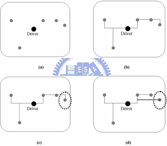
Two heuristic methods are proposed in [20]. The first heuristic method (H1) contain three steps: (1) A rectilinear Steiner minimal tree (RSMT) is constructed for all sinks;

(2) the radius-ratio of each sink is computed; (3) rerouting the sink with a direct path is performed if its radius ratio is larger than a given α, where α is a user-specified pa-rameter. Figure 1-7 is an example of first heuristic method (H1). The second heuristic method (H2) seeks a shortest path tree (SPT) as a basis and tries to further improve the wire length while relaxing the radius-ratio. The BOI-style edge addition and re-moval procedures in [24] are employed while keeping track of the radius ratio.

(a) (b)

(c) (d)

Figure 1- 7: An example of the first heuristic method (H1). (a) The routing problem of a driver

and five sinks; (b) A RSMT is constructed; (c) The radius ratio for each sink is computed, and the

radius ratios of the rightmost sink is too large (radius-ratio > α); (d) Rerouting the rightmost sink

1.4 Motivation

Most previous performance-driven Steiner tree algorithms do not consider obsta-cles during Steiner tree construction. A-Tree algorithm [4] analyzes the delay of

dis-tributed RC circuit, and then declares that delay upper bound is minimal if the tree is an SPT (shortest path tree with minimal path length from driver to sink) and an OST (optimal Steiner tree with minimal wire length) simultaneously. Therefore, A-Tree algorithm maintains an SPT, while steadily approaching an OST. However, it is hard to identify an SPT or an OST under obstacle-avoiding constraint because the obstacles may induce detoured routing. Thus, in this thesis, we propose an algorithm for the performance-driven obstacle-avoiding rectilinear Steiner tree (PDOARST) problem for modern SOC designs.

1.5 Contributions

In this thesis, we present a simple yet effective algorithm called critical-trunk based delay minimization algorithm. Since it is hard to seek a Steiner tree approach-ing a pure SPT or OST under obstacle-avoidapproach-ing constraint, the radius ratio based ap-proach in [20] is exploited in the proposed to minimize maximum signal delay. The sinks whose radius is longer than the predefined threshold value are pre-routed and these pre-routed paths are called critical trunks. Finally, we apply the proposed redi-rect mechanism to improve sink slack time to meet timing constrain.

For the PDOARST problem, we have the following distinguished features:

(1) The two-stage tree construction approach (MST construction followed by the transformation of MST to OASG) has a defect of large execution time. Instead of the two-stage tree construction approaches adopted by previous works on OARSMT problem [9][10], routing algorithm is employed to seek the tree in this work. Thus, the flexibility to add timing-related control in routing process is in-creased. Experiments reveal that the proposed PDOARST algorithm is even faster than previous OARSMT algorithms.

The first step of the proposed algorithm is to build an OASG. For the case with obstacles, we can capture the locations of obstacles by OASG. On the other hand, the OASG would become a normal spanning graph which contains all the pins for the case without obstacles.

(3) Since the main objective of performance-driven Steiner tree is to reduce the WNS, the proposed algorithm first constructs a Steiner tree with minimal delay. Then WNS is reduced by the proposed redirect mechanism. The main idea of redirect mechanism is to disconnect the sink with WNS, and then reconnect this sink on the OASG. Hence, by exploiting OASG, obstacles do not need to be considered during the process of redirect mechanism. As a result, the proposed redirect mechanism fast improves sink slack a lot.

As compared with OARSMT, experiments show that the average reduction rates of WNS and worst delay (WD) 81.52% and 28.42%, respectively. Furthermore, as re-gards the comparison to a timing-driven Steiner tree algorithm called C-Tree [21], the proposed algorithm achieves an average 53.92% reduction rate of WNS and an aver-age 15.61% reduction rate of wire length, running 27.69X faster than C-tree. In addi-tion, the proposed algorithm can be employed to solve OARSMT problem efficiently with a little modification. Extensive experiments show that the proposed algorithm identifies almost the same wire length as all state-of-the-art OARSMT algorithms, running 4.17X and 1.16X faster than [10] and [16].

1.6 Thesis Organization

The rest of this thesis is organized as follows. Chapter 2 formulates the PDO-ARST problem and describes some preliminaries. Chapter 3 presents our PDOPDO-ARST algorithm. Chapter 4 extends our algorithm to solve the OARSMT problem. Chapter 5 reports the experimental results. Finally, we conclude our work in Chapter 6.

Chapter 2 Problem Formulation and

Preliminaries

2.1 Problem Formulation

Some terminologies and their properties are first introduced.

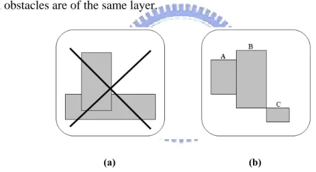
(1) Obstacle: An obstacle may be an IP-core, macro cell or pre-routed wire. Every obstacle is a rectangle, and cannot overlap the other obstacles. Two obstacles can abut at one side or a corner. For instance, in Fig. 2-1(b), obstacle B abuts obstacle

A at its left side, while abutting obstacle C at its bottom right corner. In addition,

all obstacles are of the same layer.

(a) (b)

Figure 2- 1: (a) Obstacles are not allowed to overlap another obstacle; (b) two obstacles can abut

at one side or a corner.

(2) Pin: Pins and obstacles are in the same layer. Pins are limited to locate on the borders of at corners of obstacles, and cannot locate within obstacles.

(a) (b)

Figure 2- 2: Pins have to locate on the boundaries or at the corners of obstacles. (a) Illegal pin

locations; (b) legal pin locations.

(3) Edge: Edges are used to connect pins and cannot intersect obstacles. It is legal to have edges on the boundaries of obstacles, as shown in Fig. 2-3(b).

(a) (b)

Figure 2- 3: Edges is allowed to run on the boundaries of obstacles but cannot intersect obstacles.

(a) Illegal edges; (b) Legal edges.

The problem definitions of PDOARST and OARSMT are as follows.

Problem: Performance-Driven Obstacle-Avoiding Rectilinear Steiner Tree (PDOARST): Given a set of pins, says P= {p1 , p2 ,p3,…..pm }, (containing driver and

sinks) and a set of obstacles, says O= {o1 ,o2 ,o3,….ok }, on a layer and timing-related

information, such as unit wire resistance, unit wire capacitance, sink output loading, driver resistance and some technology parameters, construct a rectilinear Steiner tree to connect all pins in P such that all edges are legal. Meanwhile, the maximal delay and worst negative slack are minimized.

Problem: Obstacle-Avoiding Rectilinear Steiner Minimal Tree (OARSMT):

Given a set of pins, says P= {p1 , p2 ,p3,…..pm }, (containing driver and sinks) and a set

of obstacles, says O= {o1 ,o2 ,o3,….ok }, on a layer, construct a rectilinear Steiner tree

Steiner tree is minimized.

2.2 Preliminaries

Preliminaries contains three parts used in this thesis – Elmore delay model, A* search algorithm and region tree algorithm.

2.2.1 Elmore Delay Model

Elmore delay model was proposed to quickly compute the signal delay of each sink with accuracy and fidelity under a tree topology [25]. More precisely, the Elmore delay model uses first-order time constant at a node as a sum of RC component. All the nodes on the circuit network are visited in this model and the Elmore delay in-volves multiplying the capacitance at the node being visited by the sum of all the re-sistances from the driver to the currently visited node. Formula (6) displays the El-more delay at node i as follows:

Delayi =

∑

× k node all k ki C R _ _ * * (6)

, where Rki*is the sum of all the resistances that are common to two paths – one from

the driver to node i and another from the driver to node k, and Ck* is the capacitance at

node k. Figure 2-4 shows an example for calculating Elmore delay. For instance, the delay at node 4 is C₁R₁ +C₂(R₁+R₂)+C₃R₁+C₄(R₁+R₂ +R₄)+C₅(R₁ +R₂).

2.2.2 A* Search Algorithm

A* search algorithm is a best-first graph search algorithm that identifies the least-cost path from a source node to the target node. It employs a function, which is denoted by f(x) and mixed with the cost from the start node to current node and the cost estimated from current node to the target node, to determine the searching order of the nodes in the graph. Formula (7) displays the cost function of A* search algo-rithm as follows. ) ( ) ( ) (x g x h x f = + (7)

, where g(x) is the accumulated cost from the start to current node x and h(x) is the estimated cost, which is usually an admissible heuristic estimation (lower bound) of the distance from node x to the target node. For routing application, h(x) might repre-sent the Manhattan distance between node x and the target node.

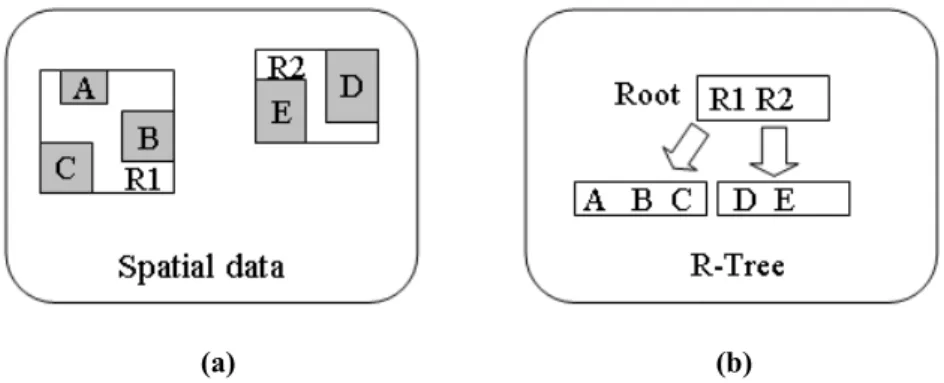
2.2.3 Region Tree (R-Tree) Algorithm

R-tree is a tree data structure used for spatial data querying. This data structure splits space by using hierarchycial minimun bounding rectangles, and that’s also the reason why this data sturcture is called “R”-Tree. More precisely, each node of R-Tree consists of a variable number of rectangles, and each rectangle stores two pieces of data. The first one is a spatial record that describes the dimensional informa-tion of this rectangle. The second one is a pointer that points to its child node. What’s more, the area of child must be included in the area of its parent.

As for how to search R-Tree, we use following R-Tree as example. For instance, we want to query how many rectangles region R1 contains. The search starts with root node, and then we will check each member in root node to find the member its area overlaps region R1. Therefore, we find member R1 in the root node. Besides, R1

points to the child node that contains three members and all the three members are included in our searching region. Hence, region R1 contains three rectangles, and the answer would is three. By this example, we could understand that the most node of R-Tree is untouched while searching, and that’s such a good property for using R-Tree as spatial querying data structure.

(a) (b)

Figure 2- 5: An example of Region Tree (R-Tree). (a) Rectangle A, B, C, D, E are the inputted

spatial data, and R1, R2 are minimum bounding rectangles generated by R-Tree; (b) How R-Tree

Chapter 3 PDOARST Algorithm

3.1 Steiner–Tree Delay Analysis

An important relation between radius (path length from driver to sink) and cir-cuit delay is observed. This relation is commonly observed in Steiner tree construction with as well as without obstacles. Figure 3-1 and 3-2 show that the fact that a long radius of a sink infers its large delay holds for both MST and SPT. It is mostly caused by the increasing number of sub-tress connecting to the large-radius path, which in-creases the downstream capacitance on this path and then the path delay. Hence, bounding the longest radius requires pre-routing these large-radius sinks. Besides, the topologies of the sub-trees subsequently growing starting at the paths, says Pds, from

the driver to the large-radius sinks have to be well controlled. From the above obser-vation, the ideal tree topology from the driver to a large-radius sink should be a trian-gle, as shown in Figure 3-3. A short sub-tree in the figure means it has less number of nodes than that of large sub-tree. Thus the sub-trees connecting a path in Pds at the

position near the driver are allowed to have longer wire length than that of the sub-trees connecting a path in Pds at the position near the sink.

Rule 1. Reduce the wire length of the sub-trees connecting a path in Pds at the position

Figure 3- 1: Relation between radius and delay in SPT. The bolded rectangle nodes on left-upper

side of two figures are the drivers. The circled and bold nodes on right-lower side of the left

fig-ure are the sinks whose radiuses are longer than 80% of the worst radius in SPT. The circled and

bold nodes on right-lower side of the right figure are the sinks whose delays are larger than 95%

of the worst delay in SPT.

Figure 3- 2: Relation between radius and delay in MST. The bolded rectangle nodes on left-upper

side of two figures are the drivers. The circled and bold nodes on right-lower side of the left

and bold nodes on right-lower side of the right figure are the sinks whose delays are larger than

95% of the worst delay in MST.

Figure 3- 3: The topology of the proposed timing-driven Steiner tree.

Along the above observation, the following important thing is how to select a sink whose radius is so large as to deserve to be well controlled. Four definitions helpful to identify large-radius sinks are proposed in the following.

Definition: Criticality threshold factor. The Criticality threshold factor (CTF) of a

SPT is defined as the ratio of its average sink delay to its worst sink delay.

Definition: Critical radius. The critical radius of a SPT is to multiply the criticality

threshold factor by the maximum radius of the SPT.

Definition: Critical sink. A sink is said to be critical if its radius is larger than the

critical radius.

Definition: Critical trunk. Critical trunk is the path on the SPT from the driver to a

critical sink.

In the proposed approach, the performance-driven Steiner tree construction is first to identify an SPT on the constructed OASG. Criticality threshold factor is then used to represent the delay characteristics of the SPT and determine the number of critical trunks to constrain the delay of critical sinks. The delay analysis on the varia-tion of the criticality threshold factor is as follows.

(1) If criticality threshold factor approaches 1, the average sink delay is almost the same as the worst sink delay, i.e., the variation of all sinks’ delays is little. The number of critical trunks needed to be pre-routed is also few, and then total wire length can be used to measure circuit performance. In this case, minimization of total wire length is the most important thing, and pre-routing critical trunks does not favor circuit performance too much because the usage of critical trunks defi-nitely increases the total wire length. Figure 3-4 displays the result of ex-press-trunk growth when the criticality threshold factor is set to be 0.854.

Figure 3- 4: An example of the critical-trunk growth (gray and bold lines) under the situation of

criticality threshold factor to be 0.854. The bold node on upper side is the driver.

(2) If the criticality threshold factor is close to 0, then the average sink delay gets much smaller than the worst sink delay. Since the variation of all sinks’ delays is significant, we need to pre-route many critical sinks to reduce the longest radius and then the maximum delay, which is usually generated by the sinks with large radius. Figure 3-5 shows the result of critical-trunk growth when the criticality threshold factor is set to be 0.473.

In summary, an SPT with large criticality threshold factor owns a nature tree to-pology suited to performance-driven Steiner tree, so it only requires little modification to reduce the worst sink delay. On the contrary, a SPT with small criticality threshold factor infers a poor tree topology for performance-driven Steiner tree.

Figure 3- 5: An example of critical-trunk growth (gray and bold lines) under the situation of

criticality threshold factor to be 0.473. The bold node on right-lower side is driver.

3.2 PDOARST Overflow

Figure 3-6 displays the flow of the proposed critical-trunk based delay minimi-zation algorithm. Each step is introduced as follows.

Figure 3- 6: Overall flow of critical-trunk based delay minimization algorithm.

(1) Step 1: traditional obstacle-avoiding spanning graph is constructed.

(2) Step 2: this step is the most crucial part of our algorithm, and the key idea is to connect the long-radius sink first. Theses pre-routed paths are called critical

trunks to signify that most of pins are reachable by visiting critical trunks and their

connected sub-trees. We first decompose every multi-pin net into several 2-pin nets by Prim algorithm, and then an SPT is constructed by incrementally routing 2-pin net on the OASG. After building the SPT, we compute the criticality thresh-old factor and then grow trunks based on this ratio. In addition, we calculate the delay penalty factor for each sink. The criticality threshold factor and delay pen-alty factor determine the Steiner tree topology in step 3. Finally, the non-trunk path is ripped up from the SPT.

(3) Step 3: all non-tree sinks are connected based on the criticality threshold factor and delay penalty factor.

(4) Step 4: all slant edges are transformed into horizontal and vertical edges and re-finement operation is employed to remove redundant edges.

the maximal delay. Furthermore, the slack time problem is considered. Redirect mechanism is used to improve sink slack time to meet the timing constrain.

Figure 3-7 displays the result of each step.

(a) (b)

(e)

Figure 3- 7: The result of every step of the proposed critictrunk based delay minimization

al-gorithm. (a) Input problem. The bold and bigger node at the right bottom corner is the driver

and other nodes are the sinks; (b) Construct OASG; (c) Grow critical trunks; (d) Sink routing; (e)

Transformation of slant edges into horizontal and vertical edges.

3.3 OASG Construction

Figure 3- 8: Overall flow of OASG construction

We apply the traditional algorithms, such as the algorithms in [9] and [16], to con-struct the OASG. The flow of OASG concon-struction is illustrated in Fig. 3-8. First, for

each vertex (a pin or an obstacle’s corner), the plane is split into four quadrants with the vertex under processing being the origin, and then edge connection is performed in each quadrant. The edge connection algorithm in [16] is employed in this thesis. In step 2, all vertices are sorted in an increasing order of the value of (x + y), and scanned by performing sweep line algorithm starting at left-bottom side towards right-upper side. Figure 3-9 shows an example of edge connection in Quadrant 1. In step 3, all vertices are sorted in an increasing order of the value of (y - x), and scanned by performing sweep line algorithm starting at right-bottom side towards left-upper side. Figure 3-10 displays an example of edge connection in Quadrant 2. Similarly, in steps 4 and 5, all vertices are sorted in a decreasing order of the values of (x + y) and (y - x), and scanned by performing sweep line algorithm starting at right-upper and left-upper sides towards left-bottom and right-bottom sides. Figure 3-11 and 3-12 show examples of edge connection in Quadrants 3 and 4, respectively.

Figure 3- 10: Step 3: Edge connection in Quadrant 2.

Figure 3- 11: Step 4: Edge connection in Quadrant 3.

Figure 3- 13: An example result of OASG construction

Another approach to construct OASG is proposed by Lin et al. [10]. Instead of connecting only one closest vertex in each quadrant, it connects as many vertices as possible to ensure that all the essential spanning edges are in the OASG. As a result, the wire length in [10] is around 2% less than that in [16] with higher edge complexity of log2n than that of logn in [9] and [16]. Since the wire length reduction rate is too small and such small wire length reduction rate is not necessarily helpful to perform-ance-driven Steiner tree problem. Besides, high edge complexity definitely highly in-creases the run time of the proposed algorithm using maze routing in constructing Steiner tree. Therefore, we use the OASG construction method in [16].

3.4 SPT Construction

An initial performance-driven Steiner tree is obtained by finding a SPT on the OASG. The SPT is identified by first constructing a complete graph only containing all pins. Then Prim algorithm is employed, starting at the driver node, to generate 2-pin nets. Since the corners of obstacles are not considered here, this stage is very fast. In the ongoing process, the effects of obstacles are considered and redundant edges are removed. Routing is accomplished by multi-source single-target maze rout-ing with the cost function of SPT-driven A* search.

3.4.1 Multi-Source Single-Target Maze Routing

To increase the flexibility of Steiner tree construction, every two-pin routing is performed by extended single-source single-target maze routing, called multi-source single-sink maze routing. The bounding box of the source and target nodes is ex-panded by a value, determined by a user-defined parameter. Then all other in-tree nodes (pins or obstacle’s corners) within the expanded bounding box are identified as source nodes. The region search is accomplished by R-Tree query to find the new source nodes. Figure 3-14 shows an example identifying new sources within the ex-panded bounding box. In the beginning of routing, all sources computes their cost us-ing A* search and then are sequentially pushed into a heap that stores incomplete routing paths. The routing path of the least cost is popped out for further propagation until reaching the target.

(a) (b)

Figure 3- 14: An example of identifying new sources. (a) The two-pin net to be routed; (b)

Bounding box and expanded bounding box for searching new sources; (c) One new source is

identified.

3.4.2 A* Search Schemes

The goal of SPT search is to find a shortest-length path from the driver to each sink. The g(x) in SPT search is the distance from the driver to current node and the h(x) in SPT search is the estimated distance from current node to the target. Figure 3-15 displays the result of performing multi-source single-target maze routing with the cost function of SPT-driven A* search.

Figure 3- 15: An example of performing multi-source single-target maze routing with the cost

function of SPT-driven A* search. The bold node on upper side is the driver.

3.5 Critical Trunk Growth

Critical trunk growth contains four stages – criticality threshold factor calcula-tion, critical trunk seleccalcula-tion, and non-critical trunk rip-up.

3.5.1 Critical Trunk Selection

According to the critical sinks identified by the above definition, critical trunks can then be specified in the SPT. Figure 3-16 shows the result of specifying critical trunks using the critical sinks.

Figure 3- 16: The result of specifying critical trunks in the SPT. The bold node on upper side is

the driver. The gray and bold lines are critical trunks. The circled and bold nodes are critical

sinks.

3.5.2 Rip-Up of Non-Critical Trunk

This stage is to remove all the paths not on the critical trunks, and all the uncon-nected sinks are left to be routed in later stage. Figure 3-17 shows a result of ripping up all non-critical trunks.

Figure 3- 17: The result of ripping up the paths not on critical paths. The bold node is the driver.

3.6 Sub-Tree Re-Routing

3.6.1 Delay Penalty Factor

During sub-tree re-routing, wire length control for the sub-tree connecting the points on critical trunks and near critical sinks is very vital. Sub-tree wire-length con-trol mechanism is accomplished by providing a factor, called delay penalty factor (DPF), which is defined for the following formula.

⎪⎩ ⎪ ⎨ ⎧ _∈ = otherwise N n R R n DPF n cr , 0 , ) ( _max (8)

, where n is the node under DPF calculation, Rn is the radius of node n on the SPT,

Rmax is the maximum radius of the SPT, and Ncr is the set of nodes on the critical

trunks. DPF(n) increases as node n∈Ncr and gets further away from the driver. This

relation satisfies the desire of reducing the wire length of sub-tree connecting a criti-cal trunk at the position closer to the criticriti-cal sink. Increased penalty factor of a node prevents from connecting the node to other node not on the critical trunk with large wire length. Delay penalty factor should not have effect for the nodes not on the criti-cal trunks, so their DPF is set to be 0. Figure 3-18 is an example of

de-lay-penalty-factor calculation.

Figure 3- 18: The example of determining delay-penalty-factor calculation.

3.6.2 Re-Routing Order and A* Search

Sub-tree re-routing applies the same two-pin net routing order as that of SPT construction, but the re-routing will be ignored if two pins of the re-routing are on the critical trunk. Re-routing is performed using multi-source single-target maze routing with delay-driven A* search cost function. Cost function f(x) is a sum of two func-tions: (1) the path-cost function g(x) and (2) an admissible heuristic estimation of the distance to the target h(x). h(x) is the traditional estimation method. The path-cost function g(x) is reinforced to consider delay effect by adding delay penalty cost to the original distance cost from the source to current node.

(

CTF

)

s DPF d d n g( )= _sn + _ds× ( )2× 1− (9) , where dsn is the distance cost from the source to node n, dds is the distance cost from

the driver to the source and CTF is the criticality threshold factor of the SPT. If the source is on a critical trunk and near the trunk’s critical sink, then the sub-tree con-necting this critical trunk at this source is imposed by high DPF upon the increase in wire length. The DPF is applied in a square form because delay is in proportion to the square of wire length. The delay penalty is finally multiplied by (1 – CTF) because a

CTF near 1 implies that little critical trunks are required and minimizing maximum

delay is achieved by minimizing total wire length.

If the source of a re-routing is on a critical trunk, the delay penalty factor of the target of this re-routing will inherit the source’s DPF after the re-routing is complete. The DPF inheritance assures further re-routing starting at current target of the specific control over wire length on the preceding source (The first source is on a critical trunk). Figure 3-19 shows the effect of DPF inheritance. At first, nodes a, b and c have their DPF of zero. After two re-routings, the DPFs of nodes a and b are set to be 0.6 and 0.2 by inheriting their source’s DPF. Then the subsequent re-routing will connect nodes b and c instead of a and c, as requested by Rule 1.

(a)

(c)

Figure 3- 19: DPF inheritance makes sure that subsequent re-routings will follow Rule 1 to

com-plete sub-tree re-routing. (a) The DPFs of nodes a, b and c initially are zero; (b) The DPFs of

nodes a and b set to be 0.6 and 0.2, respectively, by DPF inheritance; (c) Subsequent re-routing

connects nodes b and c instead of a and c to achieve a better delay at critical sink.

3.7 Transformation of Slant Edges into Rectilinear Edges

This stage is to transform all edges into horizontal and vertical edges. Besides, some refinement by removing redundant edges is also performed in this stage. Figure 3-20 shows an example of transformation of slant edges into rectilinear edges and Fig. 3-21 shows two examples of redundant edge removal.

Figure 3- 21: Two examples of redundant edge removal.

3.8 WNS Reduction

Another issue for performance-driven Steiner tree is to reduce the WNS if the slacks of some nodes are negative. WNS reduction iteratively identifies the WNS sink, removes its routing, and re-routes the sink to get an improved delay. Removing the routing of the WNS sink is to disconnect the WNS sink from the Steiner tree by re-moving the routing paths between the WNS sink and its first upper stream node that is a sink or a corner of an obstacle. Re-routing the WNS sink first requires selecting a target. To take full advantage of the previously constructed OASG, the node with minimum delay and spanning edges on the OASG is set as the best node to connect the WNS sink by spanning edge. After re-routing is complete, the edges in the re-routing result are transformed to rectilinear edges and timing is analyzed again to see if WNS reduction should end. During the WNS reduction iteration, a sink might be routed to connect its old first upper stream node. In this case, further WNS re-duction will remove the paths between the sink and its second rather than first upper stream node to disconnect the sink from the Steiner tree. WNS reduction iterates until all negative slacks are solved or runtime has reaches a threshold value. Figure 3-22 shows the flow of WNS reduction. The states of WNS reduction iterations are

re-corded and the Steiner tree is restored to the state with best result as the final Steiner tree. Figure 3-23 shows an example of WNS reduction.

Figure 3- 22: The flow of redirect mechanism to reduce worst negative slack

(a)

(c)

(d)

Figure 3- 23: An example of one round of redirect mechanism (a) find WNS sink (b) disconnect

WNS sink in tree (c) find the best node to connect WNS sink on OASG (d) turn slant edge into

Chapter 4 Extension to OARSMT Problem

The proposed algorithm is very flexible and can be employed to solve OARST problem very well with little modification. Critical trunk growth and WNS reduction are not required in OARST problem. Besides, critical trunk growth is not necessary and the DPF of every node is set to be 0. All timing-related constraints are removed. For A* search, g(x) indicates the distance cost from the source to current node and h(x) is the estimated distance cost from current node to the target. The entire flow con-tains – OASG construction, net decomposition into multiple two-pin nets, sub-tree routing on OASG, and transformation of edges into rectilinear paths, as shown in Fig. 4-1.

Chapter 5 Experimental Results

The proposed algorithm is implemented using C++ language on two platforms. The first platform is on a PC with 21.GHz AMD Athlon 64 Dual Core Processor CPU and 1.5GB memory. The second platform is on a workstation SUN UltraSPARC-III with 1.2GHz CPU and 4GB.

5.1 OARSMT Problem

Total 12 benchmarks (RC01-RC12) are used in OARSMT problem. The binary programs of [9], [10], [16] and ours are running on platform 1. Table 5.1 lists the tree wire length and required run time, where AVI is referred to as the average improve-ment rate. The average wire-length improveimprove-ment rates of the proposed OARSMT al-gorithm over [9], [10] and [16] are 1.0033, 0.9785 and 0.9997. The proposed algo-rithm achieves almost the same wire length as previous works. However the proposed algorithm outperforms in run time with the average run-time improvement rates of 4.7900, 4.1690 and 1.1617 as compared with those in [9], [10] and [16], respectively.

Platform 1 The comparison among [9], [10], [16] and our OARSMT

WL (um) Runtime (s)

Test Cases #Pin #

Ob-stacle [9] [10] [16] Ours [9] [10] [16] Ours

RC01 10 10 27,730 26,900 27,540 26,810 0.01 0.01 0.01 0.01 RC02 30 10 42,840 42,210 42,030 42,280 0.01 0.01 0.01 0.01 RC03 50 10 56,440 55,750 56,070 56,160 0.01 0.01 0.01 0.01 RC04 70 10 60,840 60,350 59,550 60,710 0.01 0.01 0.01 0.01 RC05 100 10 76,970 76,330 76,320 77,330 0.02 0.01 0.01 0.01 RC06 100 500 86,403 83,365 87,432 86,299 0.27 0.11 0.08 0.06 RC07 200 500 117,427 113,260 117,855 116,801 0.39 0.13 0.07 0.06 RC08 200 800 123,366 118,747 124,852 123,004 0.56 0.30 0.15 0.09

RC09 200 1,000 119,744 116,168 120,554 120,062 0.72 0.38 0.24 0.15

RC10 500 100 171,450 170,690 168,859 170,600 0.23 0.19 0.03 0.03

RC11 1,000 100 238,111 236,615 235,795 238,905 0.64 0.86 0.08 0.10

RC12 1,000 10,000 843,529 789,097 852,401 858,310 44.48 58.46 3.97 2.89

AVI 1.0033 0.9785 0.9997 1 4.7900 4.1690 1.1617 1

Table 5- 1: The comparisons of tree wire-length and execution run-time among [9], [10], [16] and our OARSMT approach

5.2 PD-OARST Problem

Since this thesis proposes the first work to construct performance-driven Steiner tree with obstacles, we compare the proposed critical-trunk based delay minimization algorithm with its OARSMT version. About the experiments about PDOARST prob-lem, the experimental environment settings are the same as that of [29]: 440 ohms for driver resistance, 0.076 ohms/um for unit wire resistance, 0.118 Ff/um for unit wire capacitance and 1 Ff for the loading capacitance of sink. As the required arrival time of each sink, the SPT discovered on the OASG is employed to calculate the delay of each sink, and then the delay of each sink is regarded as its required arrival time. The twelve benchmarks (RC01–RC12) for OARSMT problem are reinforced to be new benchmarks (RC01_T–RC12_T) with timing information. Table 5-2 compares the routing results of the proposed critical-trunk based delay minimization algorithm and the OARSMT algorithm (simplified version of the performance-driven algorithm), where WL is total wire length, WD is the worst delay, and AVI is the average im-provement rate.

The average wire-length and run-time increasing rates are 9.15% and 164.04%, respectively. The significant drop in execution speed is primarily caused by the com-putation of every node’s DPF and sub-tree re-routing. The encouraged results are the 28.42% average WD reduction rate and the 81.52% average WNS reduction rate.

Re-garding the run-time efficiency as compared to the algorithms without considering timing issue in [9], [10] and [16], the proposed critical-trunk based delay minimiza-tion algorithm is quite effectively, with 1.7031, 1.3206 and 0.6599 average run-time improvement rates.

Platform 1 Our OARSMT Our critical-trunk based delay minimiza-tion algorithm Test Cases WL (um) WD (ps) WNS (ps) Runtime (s) WL (um) WD (ps) WNS (ps) Runtime (s) RC01_T 26810 3709.40 -1718.31 0.01 29140 3383.64 -635.77 0.01 RC02_T 42280 4757.91 -1709.67 0.01 45170 4122.45 -297.44 0.01 RC03_T 56160 8906.42 -2851.82 0.01 60710 5694.13 -909.96 0.01 RC04_T 60710 8124.20 -3027.85 0.01 67000 5480.31 -576.47 0.01 RC05_T 77330 11690.13 -4568.54 0.01 87040 7039.76 -68.56 0.01 RC06_T 86299 10658.59 -368.31 0.06 89835 8686.66 0.00 0.11 RC07_T 116801 13450.84 -1114.31 0.06 121651 11399.44 0.00 0.17 RC08_T 123004 16169.90 -3143.81 0.09 129842 11239.62 0.00 0.29 RC09_T 120062 20957.15 -6118.16 0.15 133148 15425.91 -2630.17 0.44 RC10_T 170600 25946.16 -11539.09 0.03 176790 16888.85 -2464.52 0.12 RC11_T 238905 36459.46 -15230.98 0.10 243990 27254.68 -6930.53 0.25 RC12_T 858310 464903.49 -311970.68 2.89 1401601 187161.48 -15665.27 27.05 AVI 0.9085 1.2842 1.8152 0.6088 1 1 1 1

Table 5- 2: The Comparison of WL (wire-length), WD (worst delay of circuit), WNS (worst nega-tive slack of circuit) and execution run-time between our OARSMT and our critical-trunk based delay minimization algorithm.

The last experiment is to compare the proposed performance-driven algorithm with another performance-driven algorithm, namely C-tree algorithm [21], as listed in Tab. 5-4. The twelve benchmarks (RC01_T–RC12_T) are processed as new bench-marks (RC01_T_NO–RC12_T_NO) by removing all obstacles since C-tree algorithm

can not consider obstacles during Steiner tree construction. The proposed perform-ance-driven algorithm averagely improves the WNS, total wire length and run time by 1.5392, 1.1561 and 27.6900 as compared with C-Tree algorithm.

Platform 2 C Tree Our critical-trunk based delay minimization algorithm Test Cases WL (um) WNS (ps) Runtime (s) WL (um) WNS (ps) Runtime (s) RC01_T_NO 28580 -214.56 0.01 28670 -154.21 0.01 RC02_T_NO 49630 -474.01 0.06 50960 -262.81 0.01 RC03_T_NO 69740 -847.29 0.17 66450 -337.86 0.01 RC04_T_NO 73590 -274.15 0.24 63580 0.00 0.01 RC05_T_NO 103560 -1186.67 0.52 89810 -110.49 0.03 RC06_T_NO 111690 -1551.37 0.39 84851 -1213.89 0.02 RC07_T_NO 155937 -2239.39 1.63 112175 -1800.11 0.06 RC08_T_NO 155588 -1670.44 1.44 124064 -759.54 0.09 RC09_T_NO 166482 -3037.44 1.62 131204 -967.19 0.08 RC10_T_NO 245220 -3695.90 11.95 182630 -3309.28 0.38 RC11_T_NO 341752 -6749.56 67.21 254992 -1160.62 1.20 RC12_T_NO 1071100 -49733.90 89.80 917981 -16794.78 0.93 AVI 1.1561 1.5392 27.6900 1 1 1

Table 5- 3: The Comparison of WL (wire-length), WNS (worst negative slack of circuit) and exe-cution run-time between C-Tree and our critical-trunk based delay minimization algorithm.

Chapter 6 Conclusions

In this thesis, we propose a critical-trunk based delay minimization algorithm. The SPT obtained on the OASG is characterized by the proposed criticality threshold factor, and the delays of all critical sinks are then minimized by delay-driven A* search using the proposed delay penalty factor. DPF inheritance follows rule 1, i.e., it makes the wire length of the sub-trees connecting a critical trunk at the position close to the driver larger than that of the sub-trees connecting the same critical trunk at the position close to the critical sink. Finally, iterative WNS reduction algorithm effec-tively reduces the WNS of benchmarks. Compared with the OARSMT version of the proposed performance-driven Steiner tree algorithms, Performance-driven algorithm achieves the 28.42% average WD reduction rate and the 81.52% average WNS reduc-tion rate while with 9.15% and 164.02% average wire-length and run-time increasing rates, respectively. Regarding the run time as compared to the algorithms without considering timing issue in [9], [10] and [16], the performance-driven algorithm is quite effectively, with 1.7031, 1.3206 and 0.6599 average run-time improvement rates. Comparison of the results of performance-driven algorithms without considering ob-stacles, the proposed algorithm averagely improves the WNS, total wire length and run time by 1.5392, 1.1561 and 27.69X faster as compared with C-Tree algorithm.

Besides, the proposed performance-driven algorithm is flexible, and can be ex-tended to process traditional OARSMT with a little modification. The OARSMT ver-sion of the proposed performance-driven algorithm speeds up Steiner tree construc-tion by 379%, 317% and 16% as compared with those in [9], [10] and [16], respec-tively, while with almost equal total wire length (average wire-length improvement rates over [9], [10] and [16] are 1.0033, 0.9785 and 0.9997).

Chapter 7 Reference

[1] J. Cong, A. Kahng, G. Robins, M. Sarrafzadeh, and C.K. Wong, “Perform-ance-driven global routing for cell based ICs”, International Conference on

Com-puter Design (ICCD-1991), pp. 14-16.

[2] J. Cong, A. Kahng, G. Robins, M. Sarrafzadeh, and C. K. Wong, “Provably good performance-driven global routing”, in IEEE Trans. on Computer-Aided

De-sign of Integrated Circuits and Systems (TCAD-1992), vol. 11, no. 6, pp. 739-752.

[3] S. Rao, P. Sadayappan, F. Hwang, and P. Shor, “The rectilinear Steiner arbores-cence problem”, Algorithmica, vol. 7, no. 2-3, pp. 277--288, 1992.

[4] J. Cong, K. S. Leung, and D. Zhou, “Performance-driven interconnect design based on distributed RC delay model”, in Proceedings of ACM/IEEE Design

Automation Conference (DAC-1993), pp.606-611.

[5] C. J. Alpert, T. C. Hu, J. H. Huang, A. B. Kahng, and D. Karger, “Prim-Dijkstra tradeoffs for improved performance-driven routing tree design”, in IEEE Trans.

on Computer-Aided Design of Integrated Circuits and Systems (TCAD-1995),

vol.14, no. 7, pp. 890-89.

[6] K. D. Boese, A. B. Kahng, B. A. McCoy, and G. Robins, “Near-optimal critical sink routing tree constructions”, in IEEE Trans. on Computer-Aided Design of

In-tegrated Circuits and Systems (TCAD-1995), vol.14, no. pp. 1417-1436.

[7] H. Hou, J. Hu, and S. S. Sapatnekar, “Non-Hanan routing”, in IEEE Trans. on

Computer-Aided Design of Integrated Circuits and Systems (TCAD-1999), vol. 18.

no. 4, pp. 436-444.

[8] J. Hu and S. S. Sapatnekar, “Simultaneous buffer insertion and non-hanan optimi-zation for VLSI interconnect under a higher order AWE model”, in Proc. of