系統晶片及奈米技術下直角史坦那樹之建構

國立交通大學

電子工程學系 電子研究所碩士班

碩 士 論 文

系統晶片及奈米技術下

直角史坦那樹之建構

Unification of

Rectilinear Steiner Tree Construction

for SoC and Nanometer Technologies

研 究 生：余彥廷

指導教授：江蕙如 博士

系統晶片及奈米技術下直角史坦那樹之建構

Unification of Rectilinear Steiner Tree Construction

for SOC and Nanometer Technologies

研究生：余彥廷

Student: Yen-Ting Yu

指導教授：江蕙如 博士

Advisor: Dr. Iris Hui-Ru Jiang

國 立 交 通 大 學

電子工程學系電子研究所碩士班

碩 士 論 文

A Thesis

Submitted to Department of Electronics Engineering & Institute of Electronics College of Electrical and Computer Engineering

National Chiao Tung University in Partial Fulfillment of the Requirements

for the Degree of Master

in

Electronics Engineering June 2009

Hsinchu, Taiwan, Republic of China 中華民國 九十八年六月

i

系統晶片及奈米技術下直角史坦那樹之建構

學生：余彥廷

指導教授：江蕙如 博士

國立交通大學

電子工程學系

電子研究所碩士班

摘 要

ii

UNIFICATION OF

RECTILINEAR STEINER TREE CONSTRUCTION

FOR SOC AND NANOMETER TECHNOLOGIES

Student: Yen-Ting Yu

Advisor: Dr. Iris Hui-Ru Jiang

Department of Electronics Engineering

Institute of Electronics

National Chiao Tung University

Abstract

The rectilinear Steiner minimal tree (RSMT) problem is essential in physical design. Moreover, the variant constraints for fabrication issues, including obstacle avoidance, multiple routing layers, layer-specific routing directions, cannot be ignored during RSMT construction for modern SoC and nanometer technologies. This thesis unifies single- and multi-layer obstacle-avoiding RSMT construction first and then extends it to consider preferred routing directions and to target timing-driven RSMT. These extensions demonstrate that our algorithm can easily be adapted to configurations. Experimental results show that our algorithm is promising and outperforms the state-of-the-art works.

iii

Acknowledgements

I would like to express my heartfelt gratitude to my advisor, Prof. Iris Hui-Ru Jiang. I’ve learned several ways to cope with a tough research problem from her guidance. She is the teacher who is willing to spend her precious time just to help you preparing your oral examination. Meanwhile, I appreciate my lab members, especially Wan-Yu Lee for her foods. Finally, I display my warmest appreciation to my parents for their love and support.

Yen-Ting Yu

National Chiao Tung University June 2009

iv

Table of Contents

Chapter 2 PROBLEM FORMULATION AND ALGORITHM ... 8

A. Delaunay Triangulation of Pins ... 10

B. Obstacle-Weighted MST on DT ... 12

C. Rectilinearization and 3D U-Shaped Pattern Refinement ... 15

D. Time Complexity Analysis ... 19

Chapter 3 EXTENSIONS ... 22

A. Preferred Directions ... 22

B. Global Routing ... 25

Chapter 4 EXPERIMENTAL RESULTS ... 26

A. SL-OARSMT ... 27 B. ML-OARSMT ... 27 C. OAPDST ... 29 Chapter 5 CONCLUSION ... 35 REFERENCES ... 36 APPENDIX ... 38

v

List of Tables

TABLE I THE COMPARISON BETWEEN RECENT WORKS ON RSMT... 6 TABLE II SL-OARSMT: THE COMPARISONS ON THE TOTAL WIRELENGTH

BETWEEN PREVIOUS WORK [6-10] AND OURS ... 26

TABLE III ML-OARSMT: THE COMPARISONS ON THE NUMBER OF VIAS,

THE TOTAL COSTS, AND CPU TIMES BETWEEN [11] AND OURS UNDER CV = 3 ... 28

TABLE IV ML-OARSMT: THE COMPARISONS ON THE NUMBER OF VIAS,

THE TOTAL COSTS, AND CPU TIMES BETWEEN [11] AND OURS UNDER CV = 5 ... 29

TABLE V OAPDST: THE COMPARISONS ON THE NUMBER OF VIAS, THE

TOTAL COST, AND CPU TIMES BETWEEN [13] AND OURS UNDER CV = 3, UCI = 1, 1≦I≦NL ... 31

TABLE VI OAPDST: THE COMPARISONS ON THE IMPACTS OF OUR

ALGORITHM ON THE TOTAL COST AND CPU TIMES UNDER CV = 3, UCI = 1, 1 ≦I≦NL ... 31

vi

List of Figures

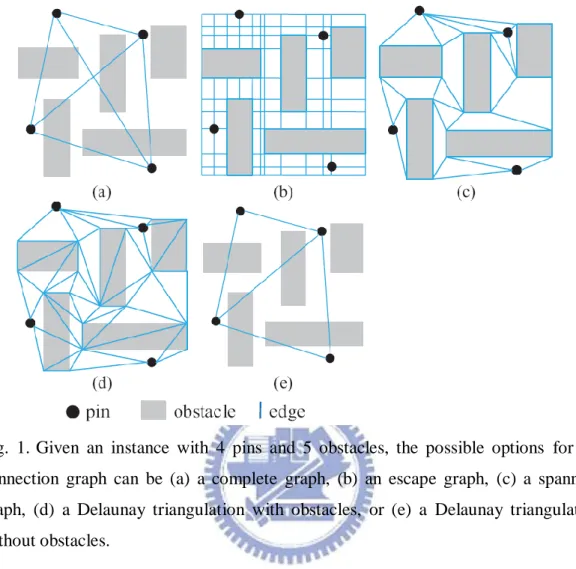
Fig. 1. Given an instance with 4 pins and 5 obstacles, the possible options for the

connection graph can be (a) a complete graph, (b) an escape graph, (c) a spanning graph, (d) a Delaunay triangulation with obstacles, or (e) a Delaunay triangulation without obstacles. ... 3

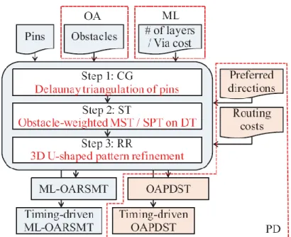
Fig. 2. We unify rectilinear Steiner tree construction. Our method can handle different

configurations, e.g., obstacle avoidance, multiple routing layers, preferred direction, and timing-driven. ... 7

Fig. 3. (a) An instance of ML-OARSMT given in [11], where Cv = 3, each grid size is 20×20 (unit)2. (b) Steps 1 and 2 of our algorithm for ML-OARSMT. (c) The corresponding 3D extended escape graph. (d) The resulting ML-OARSMT. ... 10

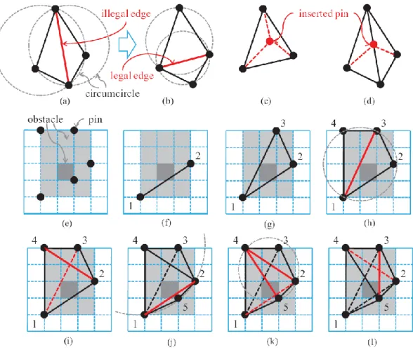
Fig. 4. (a)-(b) During DT construction, an illegal edge in is flipped into a legal one.

(c)-(d) The inserted pin may be located inside one triangle or on the boundary of two triangles. (e) The pins and obstacles in the instance given in Fig. 3(a) are projected to the pseudo plane. (f)-(l) Step-by-step DT construction for the instance given in Fig. 3(a). The number attached beside each pin indicates its order to be included in DT. Please note that the edges between pins and the initial large triangle are not shown. ... 12

Fig. 5. The obstacle penalty is counted for two pins located on the same layer. (a)

Z-shaped routing can avoid obstacle penalties. (b) The obstacle completely passes through the bounding box, and its obstacle penalty is computed as the smaller detour. .. 14

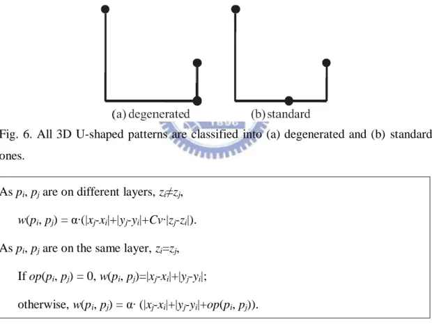
Fig. 6. All 3D U-shaped patterns are classified into (a) degenerated and (b) standard

ones. ... 14

Fig. 7. Several cases for 3D U-shaped pattern refinement. (s: Steiner-vertex) ... 15 Fig. 8. (a) The ML-OARSMT for Fig. 3(a) generated by [11] is of cost 326. It has a

degenerated pattern, marked by bold lines. (b) The refined tree has a complicated standard pattern and an obstacle around. (c) The resulting tree is of cost 269. ... 15

vii

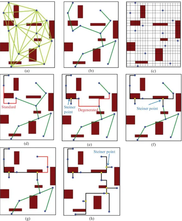
Fig. 9. An instance of SL-OARSMT. (a) Step 1: Delaunay triangulation for pins on a

pseudo plane. (b) Step 2: The obstacle-weighted MST. (c)-(h) Step 3:Rectilinearization and 3D U-shape refinement, where (c) is the escape graph, (d)-(g) are intermediate trees,

and (h) is the resulting SL-OARSMT. ... 17

Fig. 10. (a) An instance of OAPDST, where Cv = 3, each grid size is 20×20 (unit)2, UCi =1 for all layers. (b)(c) The corresponding DT, obstacle-weighted MST, and 3D extended escape graph. (d) The resulting OAPDST without refinement. (e) The resulting OAPDST with refinement. ... 21

Fig. 11. (a) Our ML-OARSMT. (b) OAPDST in [13]. (c) The refined tree of (b)... 23

Fig. 12. Degenerated cases for 3D U-shaped pattern refinement in OAPDST. ... 24

Fig. 13. (a) The SL-OARSMT of sl-rc6. (b) The SL-OARSMT of sl-rc9. ... 32

Fig. 14. The ML-OARSMT of ml-ind2 under Cv = 3. (a) The DT without illegal edges. (b) The MST. (c)-(g) Layers 2-6, respectively. (h) All pin-vertices are projected onto a pseudo plane, without showing the obstacles. ... 33

Fig. 15. The OAPDST of ml-ind2 under Cv = 3. (a) The DT with illegal edges. (b) The MST. (c)-(g) Layers 2-6, respectively. The odd (even) layers allow vertical (horizontal) edges. Some line segments are at obstacle boundaries; they are feasible according to the problem formulation. (h) All pin-vertices are projected onto a pseudo plane, without showing the obstacles. ... 34

Fig. 16. The timing driven OAPDST of ml-ind2 under Cv = 5. DT is the same as Fig. 15 (a). (a) The SPT. (b)-(f) Layers 2-6, respectively. The even (odd) layers allow vertical (horizontal) edges. Some line segments are at obstacle boundaries; they are feasible according to the problem formulation. (g) All pin-vertices are projected onto a pseudo plane, without showing the obstacles. ... 39

1

Chapter 1

INTRODUCTION

Rectilinear Steiner minimal tree (RSMT) construction has been extensively studied and considered as a fundamental problem in physical design. An RSMT is a tree of rectilinear edges connecting a given set of points possibly through some extra (i.e., Steiner) points with minimum total wire length; it is frequently performed for interconnect estimation during floor planning, placement, and routing stages. To make the estimation practical, we shall consider the fabrication issues for modern SoC and nanometer process technologies. Advanced nanometer technology offers an abundance of routing layers, e.g., 11 layers in 65 nm [1], and normally assigns a preferred routing direction to each layer; on the other hand, a large-scale SoC design often contains a tremendous number of obstacles. If timing is the main concern, the objective could be changed to minimize the path length from a designated source point to the rest.

However, even the simplest case, the RSMT problem without considering obstacle avoidance (OA), multiple layers (ML), preferred direction (PD) constraints, has been proven to be NP-complete [2]. Due to the high complexity and frequent usage, it is desired to construct an RSMT with these constraints of good quality in reasonable runtime.

A 2:1 performance bound of minimum spanning tree (MST) to RSMT for general graphs can be applied to these variations. Thus, existing approaches for RSMT typically contain three steps:

1) Connection graph generation (CG): Step 1 generates a connection graph to connect all pins. (Obstacle boundaries can also be included.) This graph contains

2

geometrical proximity information among pins (and obstacle boundaries, or not). It can be a complete graph, a spanning graph, an escape graph [3], or a Delaunay triangulation (DT) [4]. Fig. 1 illustrates these possibilities for a planar instance with 4 pins and 5 obstacles. Fig. 1(a) shows the corresponding complete graph where vertices represent pins and each edge reflects the wirelength between the related two pins with obstacle consideration. Fig. 1(b) shows the corresponding escape graph where lines are stretched horizontally and vertically along pins and the corners of obstacles, and the intersection of any two lines contributes a vertex. Fig. 1(c) shows the corresponding spanning graph where vertices represent pins and the corners of obstacles, and two vertices are connected if there is no other vertex inside or on the boundary of the bounding box of the two vertices, and there is no obstacle inside the bounding box of the two vertices [9], [11]. Fig. 1(d) shows the corresponding DT where vertices represent pins and the corners of obstacles, and the circumcircle of each triangle does not contain any other vertex. In addition, the corners of obstacles may be not included in DT to reduce the complexity of the connection graph, as shown in Fig. 1(e).

2) spanning tree construction (ST): Step 2 constructs a minimum spanning tree (MST) over all pins based on the connection graph. If the connection graph includes the corners of obstacles, the MST is obstacle-avoiding (all tree edges bypass obstacles). Otherwise, it is obstacle-weighted (tree edges may run through obstacles, but the impacts of obstacles are considered into edge weights), or mixed (tree edges are obstacle-weighted first and then obstacle-avoiding). If the goal is to construct a timing-driven RSMT, the spanning tree can be the shortest path tree (SPT) on the connection graph instead and is built up by Dijkstra’s shortest path algorithm.

3

Fig. 1. Given an instance with 4 pins and 5 obstacles, the possible options for the connection graph can be (a) a complete graph, (b) an escape graph, (c) a spanning graph, (d) a Delaunay triangulation with obstacles, or (e) a Delaunay triangulation without obstacles.

3) Rectilinearization and refinement (RR): Step 3 transforms the spanning tree into a rectilinear Steiner tree and refines the total cost. If the spanning tree is obstacle-weighted, the edges intersecting obstacles are fixed during rectilinearization. The total cost includes wirelength and vias. Planar U-shaped pattern refinement is usually applied. In addition, if the connection graph is a Hanan grid or an escape graph, some works merge steps 2 and 3 into one.

As listed in TABLE I, we compare the configurations provided and the techniques used in each step for the state-of-the-art works and ours.

Recently, most of research endeavors have focused on single-layer obstacle-avoiding RSMT (SL-OARSMT) [6], [7], [8], [9], [10]. Among them, [9]

4

produced the best results; the breakthrough done in [9] was to include more “essential edges” into their spanning graph. The essential edge introduced by [9] can directly connect two pins without obstacles inside their bounding box and then lead to more desirable solutions. [11] then extended [9] to construct a 3D spanning graph and solved the multi-layer variation; so far, it has been the first one and only one work handling multi-layer obstacle-avoiding RSMT (ML-OARSMT). [11] projected vertices between layers and within layers to link the spanning graphs for adjacent layers together. The projection reflects the usage of vias. Even so, it seems somewhat indirect to include the information of preferred directions into their 3D spanning graph.

[12] first included preferred directions into RSMT but ignored obstacles. [13] first attempted to combine all of these issues into RSMT construction and formulated the obstacle-avoiding preferred direction Steiner tree problem (OAPDST). In addition, [13] directly constructed a rectilinear MST over a 3D improved escape graph. However, the MST was not further refined, so the solution quality may be limited. Each work listed here focused on only one specific configuration and cannot easily be adapted to other configurations.

As shown in Fig. 2, in this thesis, we generalize an approximation algorithm which is a preliminary version announced in [14], [15] to unify the tree construction. Steps 1 and 2 construct an obstacle-weighted MST/SPT on the DT of pins only. Step 3 rectilinearizes each tree edge on a 3D extended escape graph and then refines it. Our innovative features include:

1) We develop a unified approach to Steiner tree construction for variant configurations.

5

geometrical information among pins and obstacles in the connection graph. We overcome the drawback by introducing potentially essential edges during DT construction and adequately associating the impacts of obstacles into edge weights.

3) We construct the DT and the obstacle-weighted MST/SPT in an efficient way since the total edge weight of the tree is not required to be exact, just expected to be correlated to the final tree. It can effectively guide step 3 how to connect pairs of pins. 4) We generalize 3D U-shaped pattern refinement. Experimental results show that our algorithm outperforms the state-of-the-art works for SL-OARSMT, ML-OARSMT and OAPDST and can extend to handle timing-driven RSMT.

Moreover, our results reveal the following findings: The guidance of the obstacle-weighted MST leads to smaller total costs and shorter runtimes, and novel 3D U-shaped refinement works well not only on our algorithm but also for previous work.

The rest of the thesis is organized as follows. Chapter 2 presents problem formulations about ML-OARSMT and how our algorithm works. The extensions of ML-OARSMT are presented in Chapter 3. Experimental results are presented in Chapter 4. Conclusions are drawn in Chapter 5. And finally, APPENDIX shows an application of our procedure.

6

TABLE I

7

Fig. 2. We unify rectilinear Steiner tree construction. Our method can handle different configurations, e.g., obstacle avoidance, multiple routing layers, preferred direction, and timing-driven.

8

Chapter 2

PROBLEM FORMULATION AND ALGORITHM

We adopt the formulation of the multi-layer obstacle-avoiding rectilinear Steiner minimal tree (ML-OARSMT) problem in [11].

Problem: Multi-Layer Obstacle-Avoiding Rectilinear Steiner Minimal Tree

(ML-OARSMT): Given the equivalent wirelength cost Cv of a via, the number Nl of

layers, a set P = {p1, p2, …, pm} of pins, a set O = {o1, o2, …, ok} of obstacles, construct a multi-layer rectilinear Steiner tree to connect all pins in P by only rectilinear edges, such that no tree edge or via intersects any obstacle in O and the total cost of the tree is minimized.

An obstacle is a rectangle on a layer, indicated by its four corner-vertices. A pin-vertex pi is a vertex (xi, yi, zi) on layer zi, while a via (xj, yj, zj) on layer zj is an edge between (xj, yj, zj) and (xj, yj, zj+1). No two obstacles can overlap with each other, but two obstacles can be point-touched or line-touched. Since an arbitrary rectilinear obstacle can be partitioned into a set of rectangles, without loss of generality, assume all obstacles are rectangular. All vertices of pins and vias must not locate inside any obstacle, but they can be at the corner or on obstacle boundaries. In addition, the single-layer obstacle-avoiding rectilinear Steiner minimal tree (SL-OARSMT) problem is a special case of ML-OARSMT as Nl = 1.

As outlined in Fig. 2, our algorithm is based on the construction-by-correction approach. Here, we use the example given in [11], depicted in Fig. 3(a), to demonstrate our algorithm. Assume Cv = 3, and each grid size is 20×20 (unit wirelength) 2.

9

DT is then constructed. During DT construction, some “illegal” edges (indicated by dotted lines) that may be essential are added. (The essential edges can lead to

more desirable solutions [11].) (see Fig. 3(b) and Fig. 4(e)-(l))

2) Step 2: An obstacle-weighted minimum spanning tree is grown up over the DT. We bias the edge weights in DT to consider obstacle penalties. (see Fig. 3(b))

3) Step 3: Each tree edge is rectilinearized on a 3D extended escape graph (see Fig. 3(c)), and is then processed by novel 3D U-shaped pattern refinement. Our ML-OARSMT for this instance is of cost 195 (=9×20+5×3). (see Fig. 3(d))

In addition, the ML-OARSMT generated by [11], as shown in Fig. 7(a), is of cost 326 (=16×20+2×3). It can be improved by our refinement method; as shown in Fig. 7(c), the refined tree is of cost 269 (=13×20+3×3). We detail each step and analyze the time complexity as follows.

10

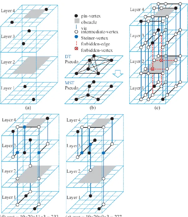
Fig. 3.(a) An instance of ML-OARSMT given in [11], where Cv = 3, each grid size is 20×20 (unit)2. (b) Steps 1 and 2 of our algorithm for ML-OARSMT. (c) The corresponding 3D extended escape graph. (d) The resulting ML-OARSMT.

A. Delaunay Triangulation of Pins

Initially, all pins are projected onto a pseudo plane, i.e., each pin-vertex is indicated by its x- and y-coordinates. If two pin-vertices are projected to the same location, they are connected by an edge. Conceptually, this pseudo plane abstracts the geometrical proximity among pins, as well as views single-layer and multi-layer trees as one.

11

For a given set P of vertices in a plane, a Delaunay triangulation DT(P) is a triangulation such that the circumcircle of each triangle does not contain any other vertex of P. A DT(P) maximizes the minimum angle of all the angles of the triangles in it, thus avoiding sliver triangles, i.e., a DT(P) tends to connect neighboring vertices.

As depicted in Fig. 4(a), during DT construction, sometimes two triangles possibly violate the definition of DT, i.e., the circumcircle of one triangle contains another vertex. The common edge of these two triangles is an illegal edge, and it is then flipped to a legal edge [4], as shown in Fig. 4(b).

Assume xmax and ymax are the maximum x- and y-coordinates of the given set of

vertices. DT construction begins with a large triangle with three vertices located at (0, 3ymax), (3xmax, 0), and (-3xmax, -3ymax) on the pseudo plane. Then, one pin at a time is

inserted. If it is located inside some triangle, it splits this triangle into three. (see Fig. 4(c)) Otherwise, it is on the common edge of two triangles, it then splits these into four. (see Fig. 4(d)) The dotted lines in Fig. 4(c)(d) are introduced by the inserted pin. If illegal edges are generated, they are then flipped into legal ones until no illegal edge remains. This process repeats until all pins are inserted. Finally, the initial large triangle and its induced edges are removed.

Normal DT construction discards these illegal edges; however, we preserve these illegal edges since they contain much more global information than legal ones and may lead to better solutions. Fig. 3(b) gives the corresponding DT of the instance in Fig. 3(a), where illegal edges are indicated by dotted lines, and legal edges are indicated by solid lines. Fig. 4(e)-(l) detail the DT construction step-by-step, where three illegal edges (indicated by dotted lines) are flipped in Fig. 4(h)(i), Fig. 4(j)(k), and Fig. 4(k)(l).

12

Fig. 4. (a)-(b) During DT construction, an illegal edge in is flipped into a legal one. (c)-(d) The inserted pin may be located inside one triangle or on the boundary of two triangles. (e) The pins and obstacles in the instance given in Fig. 3(a) are projected to the pseudo plane. (f)-(l) Step-by-step DT construction for the instance given in Fig. 3(a). The number attached beside each pin indicates its order to be included in DT. Please note that the edges between pins and the initial large triangle are not shown.

B. Obstacle-Weighted MST on DT

As shown in Fig. 3(b), after the DT is constructed for the projected pins on a pseudo plane, the obstacle-weighted minimum spanning tree is constructed based on Kruskal’s algorithm [5]. (Another option is Prim’s algorithm [5].)

The conventional construction-by-correction approach does not include the geometrical information of obstacles in the connection graph. To overcome this

13

drawback, we encode the obstacle penalties to edge weights of DT(P). Because DT(P) contains potentially essential edges and its edge weights include the obstacle information, DT(P) possesses the global geometrical information among pins and obstacles.

On the other hand, the MST is used to guide step 3 how to connect pins. The edge weight is not required to be exact, just expected to be correlated to the cost of the final RSMT. Hence, we use a simple and fast, yet effective, formula to estimate the impact of obstacles. The obstacle penalty op(pi, pj) between two pins pi and pj located on the same layer is simplified from [8], where only the obstacles completely passing through the bounding box between pi, pj horizontally or vertically are counted. Fig. 5 shows two examples for obstacle penalty computation. The pair of pins in Fig. 5(a) has no obstacles completely passing through their bounding box. If Z-shaped routing is applied, there is no routing overhead. Hence, their obstacle penalty equals zero. On contrast, in Fig. 5(b), one obstacle crosses over the bounding box of the given pair of pins. The detour incurs either 2l1 or 2l1 penalty, so their obstacle penalty can be the

smaller one.

In addition, we introduce a parameter α to further reflect the congestion of obstacles; in our experiments, α is computed by the density of obstacles. When two pins are located at the same layer with nonzero obstacle penalty or at different layers, the parameter α is used to magnify their distance. The edge weight w(pi, pj) is computed as follows.

14

Fig. 5. The obstacle penalty is counted for two pins located on the same layer. (a) Z-shaped routing can avoid obstacle penalties. (b) The obstacle completely passes through the bounding box, and its obstacle penalty is computed as the smaller detour.

Fig. 6. All 3D U-shaped patterns are classified into (a) degenerated and (b) standard ones.

As pi, pj are on different layers, zi≠zj,

w(pi, pj) = α∙(|xj-xi|+|yj-yi|+Cv∙|zj-zi|). As pi, pj are on the same layer, zi=zj,

If op(pi, pj) = 0, w(pi, pj)=|xj-xi|+|yj-yi|;

otherwise, w(pi, pj) = α∙ (|xj-xi|+|yj-yi|+op(pi, pj)).

Although we estimate the obstacle penalties in a simple way, our results reveal that steps 1 and 2 are necessary, and they can give a good guidance for step 3.

15

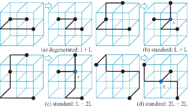
Fig. 7. Several cases for 3D U-shaped pattern refinement. (s: Steiner-vertex)

Fig. 8.(a) The ML-OARSMT for Fig. 3(a) generated by [11] is of cost 326. It has a degenerated pattern, marked by bold lines. (b) The refined tree has a complicated standard pattern and an obstacle around. (c) The resulting tree is of cost 269.

C. Rectilinearization and 3D U-Shaped Pattern Refinement

Based on the guidance of the obstacle-weighted MST, each MST edge is rectilinearized and then refined if a 3D U-shaped pattern is found. Rectilinearization

16

and 3D U-shaped pattern refinement are compounded into one operation and are iteratively applied edge-by-edge. By doing so, the refinement done for early edges can benefit consequent edges, thus our refinement does not always hurt runtimes. In addition, the MST edges are processed in a random order.

Rectilinearization is performed on a 3D extended escape graph based on Dijkstra’s shortest path algorithm [5]. We extend the planar escape graph [3] to a 3D one as follows. A 3D extended escape graph is constructed by stretching lines from all pin-vertices and the corner-vertices of all obstacles along x-, y-, and z-axes, where the line segments intersecting or passing through obstacles are prohibited to be used. Fig. 3(c) shows the 3D extended graph for the instance in Fig. 3(a). To make the implementation flexible, we adequately associate forbidden flags to the vertices inside obstacles and at obstacle boundaries.

By extending the proof done in [3], we can prove by induction that at least one optimal solution of ML-OARSMT is embedded in the 3D extended escape graph. This fact holds even if the via cost and the number of layers vary. Hence, the 3D extended escape graph does not keep our solution away from optimality. On the other hand, the proof of the 2:1 performance bound of MST to SMT for general graphs can be applied here [5].

When a tree edge is rectilinearized and connected to the partially constructed rectilinear Steiner tree, a U-shaped pattern may be formed. We generalize U-shaped pattern refinement from 2D to 3D cases. Here, we only consider the U-shaped patterns that can potentially be optimized. We have the following theorem for U-shaped patterns without obstacles inside or around.

17

Fig. 9.An instance of SL-OARSMT. (a) Step 1: Delaunay triangulation for pins on a pseudo plane. (b) Step 2: The obstacle-weighted MST. (c)-(h) Step 3:Rectilinearization and 3D U-shape refinement, where (c) is the escape graph, (d)-(g) are intermediate trees, and (h) is the resulting SL-OARSMT.

Theorem: A 3D U-shaped pattern is formed by at least three vertices (pin-vertices

and/or Steiner-vertices). It can be either degenerated if the middle vertex is located at one turning corner of the U or standard if the middle vertex is located within the

18

middle segment of the U.

Proof Sketch: If there is no obstacle inside or around a U-shaped pattern, a 2-vertex

U-shape never occurs because rectilinearization is performed based on Dijkstra’s shortest path algorithm. If there are obstacles inside, the 2-vertex U-shaped pattern results from detours. Thus, a U-shaped pattern has at least three vertices.

A U-shaped pattern with 4 or more vertices can be decomposed into several smaller ones. For a 3-vertex U-shaped pattern, only the location of the middle vertex may vary. Moreover, the middle vertex cannot be located within one of two I-shaped segments of the U. In this case, this 3-vertex U-shaped pattern is composed of one I-shaped segment plus a 2-vertex U-shaped pattern. As mentioned above, a 2-vertex U-shaped pattern never occurs. Hence, the middle vertex can be located either at one turning corner of the U or within the middle segment of the U.

1) Degenerated U-shape: The middle vertex is located in one turning corner of U. (see Fig. 6(a)) This type can be identified by one I-shaped segment plus one or more L-shaped segments. The refinement can be applied only when three vertices are located in the same plane, i.e., they have the same x-, y-, or z-coordinate. The L-shaped segments of the U can then be rerouted for cost reduction.

2) Standard U-shape: The middle vertex is located within the middle segment of the U. (see Fig. 6(b)) This type can be identified by several L-shaped segments plus several L-shaped segments. The L-shaped segments of a standard one can be ripped-up and then rerouted from these vertices to their Steiner-vertex. (The optimal location of the Steiner-vertex is at the median of the coordinates of these three vertices.)

19

examples for 3D U-shaped pattern refinement. Please note that our classification is complete. Fig. 8 shows the instance in Fig. 3(a) can be further improved by fixing one degenerated pattern plus one standard U-shaped one. The cost is reduced from 326 to 269. In addition, for this case, our algorithm can generate the tree in Fig. 3(d) of cost 195, even without refinement.

For easier visualization, Fig. 9 demonstrates a planar example with 12 pins and 8 obstacles; as mentioned in Section II, SL-OARSMT is a special case of ML-OARSMT. Fig. 9(a) depicts the corresponding DT, where illegal edges are also included. Then, based on the edge weight defined in Section III.B, Fig. 9(b) shows the corresponding MST. Fig. 9(c) shows the corresponding escape graph. Based on the MST in Fig. 9(b), rectilinearization and refinement starts from an edge randomly selected, say the edge at the up-left corner in this case. As shown in Fig. 9(d), after an edge is rectilinearized, a standard U-shaped pattern is found and refined. Fig. 9(e) shows a degenerated U-shaped pattern. It can be seen that if there are obstacles around a U-shaped pattern, e.g., Fig. 9(d)(g), the Steiner-vertex might have to be shifted accordingly; even so, we still can improve the total cost. (see Fig. 9(e)(h)) If the refined pattern has worse cost, the original one retains.

D. Time Complexity Analysis

Let n=m+4k for an instance with m pins and k obstacles. Step 1 takes O(mlgm) time for DT construction [4]; step 2 takes O(m(lgm)2) time for Kruskal’s algorithm; step 3 takes O(n3) time for the 3D extended escape graph construction, Dijkstra’s algorithm, 3D U-shaped pattern refinement. As mentioned in Section III.B, steps 1 and 2 can effectively guide step 3, and they have low time complexities, so they are worthwhile. Although 3D U-shaped pattern refinement in step 3 has a high time

20

complexity, it can be expected to produce good solutions.

Compared with [11], steps 1 and 2 of our algorithm have relatively low time complexities, and step 3 has the same order complexity. Since the time complexities are the same, it would be a good decision to take time on sophisticated refinement.

21

Fig. 10.(a) An instance of OAPDST, where Cv = 3, each grid size is 20×20 (unit)2,

UCi =1 for all layers. (b)(c) The corresponding DT, obstacle-weighted MST, and 3D extended escape graph. (d) The resulting OAPDST without refinement. (e) The resulting OAPDST with refinement.

22

Chapter 3

EXTENSIONS

A. Preferred Directions

In this section, we shall demonstrate the flexibility of our algorithm. As shown in Fig. 2, our algorithm for ML-OARSMT can easily be extended to consider preferred directions. We adopt the formulation of the obstacle-avoiding preferred direction Steiner tree (OAPDST) problem in [13].

Problem: Obstacle-Avoiding Preferred Direction Steiner Tree (OAPDST): Given

the equivalent wirelength cost Cv of a via, the number Nl of layers, a set P = {p1,

p2, …, pm} of pins, a set O = {o1, o2, …, ok} of obstacles, the layer-specific routing cost UCi, 1≦i≦Nl, the PD constraints, construct a Steiner tree to connect all pins in

P, such that no tree edge or via intersects any obstacle in O and the total cost of the

tree is minimized.

The definitions and restrictions of an obstacle, a pin-vertex, a via are the same as those in Section II. Here, a routing layer I has a specific routing cost UCi, the unit cost of wires in layer i. Without loss of generality, assume the PD constraints as follows: the odd (even) layers only allow vertical (horizontal) edges [12, 13].

To adapt our algorithm for ML-OARSMT to OAPDST, we apply simple and effective modifications to the DT, the 3D extended escape graph, and 3D U-shaped pattern refinement.

1) The DT: For each edge, the part of edge weight contributed by the Manhattan distance is multiplied by UCi, and α is changed to be a function of obstacles and UCi. For the edge between pi and pj (located at layers zi and zj), the UCi for vertical (horizontal) segments is the minimum value among vertical (horizontal) layers from

23

layer min(zi, zj)-1 to layer max(zi, zj)+1.

24

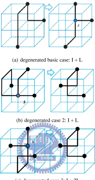
(a) degenerated basic case: I + L

(b) degenerated case 2: I + L

(c) degenerated case 3: I + 2L

Fig. 12.Degenerated cases for 3D U-shaped pattern refinement in OAPDST. 2) The 3D extended escape graph: The horizontal (vertical) edges on odd (even) layers are removed. (They are forbidden.) The edge cost on layer i is magnified by

UCi, 1≦i≦Nl.

3) 3D U-shaped pattern refinement: Considering the PD constraints, a Steiner-vertex can only connect vias either with vertical edges or with horizontal edges. For a given U-shaped pattern formed by three vertices, the median of their coordinates may not be valid for a Steiner-vertex. However, the median point still can be a reference point to reroute the L-shaped segments on the pattern, so the strategy is

25

the same as that in ML-OARSMT.

Fig. 11(a) shows the instance given in [13]; assume Cv = 3, each grid size is 20×20 (unit wirelength)2, UCi =1 for all layers. Fig. 11(b)(c) show the corresponding DT, the obstacle-weighted MST, and the 3D extended escape graph. Fig, 10(d)(e) depicts the resulting OAPDST without refinement (cost = 233 (=10×20+11×3)), with refinement (cost = 227 (=10×20+9×3)), respectively. Fig. 12(a) shows the corresponding ML-OARSMT generated by our algorithm, cost = 218 (=10×20+6×3); it can be viewed as the lower bound of the cost of OAPDST. Fig. 11(b) shows the OAPDST given in [13], cost = 281 (=13×20+7×3), where a standard pattern is highlighted by bold lines. After refining this pattern, we can obtain a better tree in Fig. 11(c), cost = 261 (=12×20+7×3). Fig. 12 lists degenerated cases for refinement in OAPDST.

B. Global Routing

To include our Steiner tree construction to global routing, we shall consider the capacity of each edge on the global routing graph. Without loss of generality, assume the net ordering is given. It can be seen that on the 3D escape graph, if the capacity of some edge is full, then this edge can be set as forbidden; otherwise, this edge can still be used. After the RSMT is constructed, the capacity of the corresponding routed edges reduces. Moreover, considering the grids on upper metal layers are larger than lower ones, we may slightly shift the lines of the3D escape graph to align their nearest grids.

26

Chapter 4

EXPERIMENTAL RESULTS

We implemented our algorithm in C++ language and executed the program on a PC with an Intel Pentium4 3.0 GHz CPU and 1 GB memory under Windows XP OS. Our results show our algorithm outperforms state-of-the-art works on SL-OARSMT, ML-OARSMT, and OAPDST. Meanwhile, our runtimes are also stable, not increasing much from SL-OARSMT to ML-OARSMT and OAPDST. In addition, the comparison between DT without and with obstacles is provided. Furthermore, the results of timing-driven RSMT are also provided.

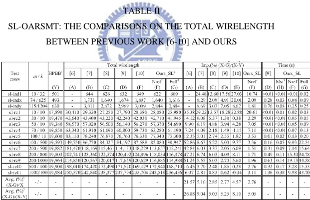
TABLE II

SL-OARSMT: THE COMPARISONS ON THE TOTAL WIRELENGTH BETWEEN PREVIOUS WORK [6-10] AND OURS

1

HPBB: The half-perimeter of the bounding box of all pin-vertices (which is a lower bound of total wirelength), and “-” refers to “not available.”

2

Ours_SL: Our algorithm for SL-OARSMT.

3

27

4

Full: All steps of our algorithm are applied.

5

Mst: Step 1 (DT) and step 2 (MST) of our algorithm are applied.

6,7

Avg. (%): Average improvement is computed by averaging (X-G)/X, and (X-G)/(X-Y) for all cases, X = A, B, C, D, E, F.

A. SL-OARSMT

For SL-OARSMT, totally 14 benchmark circuits were provided by [8]; the first 3 from industry, the rest from [6]. We compared our algorithm with those presented in [6], [7], [8], [9], [10]. The results of [6] and [8] are quoted from their papers; those of [7] are quoted from [8]; those of [9] and [10] were conducted on our platform using their binary codes. (In addition, the parameter α was set to [0.50, 1.30] depending on the congestion.) As listed in TABLE II, considering the differences from the half-perimeter of the bounding box of all pins (which is a lower bound of the optimal solution), our algorithm achieved average 5.03% up to 26.88% improvement on wirelength over them. Moreover, we had the best results for 12 out of 14 cases. Fig. 13 shows the resulting SL-OARSMTs of sl-rc6 and sl-rc9. Without refinement, on average, we still have a small win to [8] and [9] on total wirelength. Novel 3D U-shaped pattern refinement worked well in planar cases and contributed 2.76% reduction on wirelength. Because our method mainly focuses on multi-layer, the overhead on runtimes for single-layer is reasonable.

B. ML-OARSMT

For ML-OARSMT, totally 10 test cases were provided by [11]. ml-ind4 and ml-ind5 simulate the environment for single-layer routing, where all pins and obstacles are located in a layer, and the upper and lower adjacent layers are entirely occupied by another two large obstacles. Fig. 14 displays the ML-OARSMT of ml-ind2 generated

28

by our algorithm as Cv = 3.

We compared our algorithm with [11]. (In addition, the parameter _ was set to

[0.70, 1.15].) As listed in TABLE III (IV), as Cv = 3 (5), the average improvements on the number of vias and total costs are 7.69% (4.76%), 2.77% (2.74%), respectively. Our algorithm has smaller total costs in 9 out of 10 cases. In addition, our algorithm always generated a smaller total cost as Cv = 3 than that as Cv = 5 for each case; it can be seen that our algorithm is indeed stable.

TABLE III

ML-OARSMT: THE COMPARISONS ON THE NUMBER OF VIAS, THE TOTAL COSTS, AND CPU TIMES BETWEEN [11] AND OURS UNDER CV = 3

1

The runtimes of [11] are quoted from the paper, generated by a 2.8GHz AMD-64 machine with 8GB memory under Ubuntu 6.06 OS. They are listed for reference because the machine is different.

2

[11]_ref: 3D U-shaped pattern refinement is directly applied to the resulting ML-OARSMT of [11]. The runtimes of [11]_ref only count for refinement and are measured on our platform.

3

Ours_ML: Our algorithm for ML-OARSMT. 3Imp. (%): Average improvement is computed by averaging (A-X)/A for all cases, X =B, C or D.

29

TABLE IV

ML-OARSMT: THE COMPARISONS ON THE NUMBER OF VIAS, THE TOTAL COSTS, AND CPU TIMES BETWEEN [11] AND OURS UNDER CV = 5

1

The runtimes of [11] are quoted from the paper, generated by a 2.8GHz AMD-64 machine with 8GB memory under Ubuntu 6.06 OS. They are listed for reference because the machine is different.

2

[11]_ref: 3D U-shaped pattern refinement is directly applied to the resulting ML-OARSMT of [11]. The runtimes of [11]_ref only count for refinement and are measured on our platform.

3

Ours_ML: Our algorithm for ML-OARSMT. 3Imp. (%): Average improvement is computed by averaging (A-X)/A for all cases, X = B, C or D.

C. OAPDST

For OAPDST, totally 10 test cases are used. 7 cases are exactly the same as those used in ML-OARSMT. We did not use ml-ind3 because it is invalid under the PD constraints. pd-ind4, pd-ind5a, pd-ind5b were modified from ml-ind4 and ml-ind5. For pd-ind4 and pd-ind5a, we inserted one empty layer right above the working layer. For pd-ind5b, we further duplicated the obstacles in the working layer onto the inserted layer. In addition, the routing cost UCi was set to 1 for all i. By doing so, we can see how worse an OAPDST can be with respect to its ML-OARSMT counterpart. (In addition, the parameter α was set to [0.70, 1.00].) Fig. 15 displays the OAPDST of ml-ind2 generated by our algorithm as Cv = 3.

30

and the program of [13], we implemented their algorithm and executed it on the same machine described above.

As listed in TABLE V, as Cv = 3, the average degradation of the total costs from ML-OARSMT to OAPDST is 6.47%, but the average speedup of CPU times is 60.18%. The average improvement of the total costs over [13] is 3.20%, while the CPU times are almost the same. Our algorithm has smaller total costs in 9 out of 10 cases.

TABLE VI compares the impacts of the obstacle-weighted MST and 3D U-shaped pattern refinement of our algorithm. It can be seen that without the guidance from the MST, on average, we may have an 8.76% degradation on the total costs, and the CPU times surprisingly become much worse (38.88% slower). Hence, steps 1 and 2 are necessary; actually, they are efficient and effective. On the other hand, although 3D U-shaped pattern refinement does not influence much on our results, it does improve the total costs of [13] by 2.66% on average. The refined results of [13] are still slightly worse than ours when refinement is turned off. Although not presented here, we have similar results for Cv = 5, and UCi ≠ 1.

31

TABLE V

OAPDST: THE COMPARISONS ON THE NUMBER OF VIAS, THE TOTAL COST, AND CPU TIMES BETWEEN [13] AND OURS UNDER CV = 3, UCI = 1,

1≦I≦NL

1

Ours_ML: Our algorithm is applied without the PD constraints; it can be viewed as the lower bound of the total cost for OAPDST.

2

Ours_PD: All steps of our algorithm for OAPDST are applied. 3Imp. (%): Average improvement is computed by averaging (X-B)/X for all cases, where X = A, C.

TABLE VI

OAPDST: THE COMPARISONS ON THE IMPACTS OF OUR ALGORITHM ON THE TOTAL COST AND CPU TIMES UNDER CV = 3, UCI = 1, 1≦I≦NL

1

Nmst: Only step 3 of our algorithm is applied, i.e., the tree is directly constructed from the 3D extended escape graph.

2

Nref: All steps of our algorithm are applied, but 3D U-shaped pattern refinement is turned off.

3

[13]_ref: 3D U-shaped pattern refinement is applied to [13].

4

32 in TABLE IV, X = D, E, F.

33

Fig. 14.The ML-OARSMT of ml-ind2 under Cv = 3. (a) The DT without illegal edges. (b) The MST. (c)-(g) Layers 2-6, respectively. (h) All pin-vertices are projected onto a pseudo plane, without showing the obstacles.

34

Fig. 15.The OAPDST of ml-ind2 under Cv = 3. (a) The DT with illegal edges. (b) The MST. (c)-(g) Layers 2-6, respectively. The odd (even) layers allow vertical (horizontal) edges. Some line segments are at obstacle boundaries; they are feasible according to the problem formulation. (h) All pin-vertices are projected onto a pseudo plane, without showing the obstacles.

35

Chapter 5

CONCLUSION

In this thesis, we solved ML-OARSMT and OAPDST by the same strategy. In addition, we also showed our method can be extended to construct timing-driven RSMTs. Previous work tackles one configuration at a time, while our algorithm can easily handle various configurations. Experimental results showed that our algorithm outperformed the state-of-the-art works. Future work includes the extensions to clock trees and manufacturability-aware trees.

36

REFERENCES

[1] The International Technology Roadmap for Semiconductors (ITRS), 2007. Available: http://www.itrs.net/

[2] M. R. Garey and D. S. Johnson, “The rectilinear Steiner tree problem is NP-complete,” SIAM J. Appl. Math., vol. 32, no. 4, pp. 826-834, 1977.

[3] J. L. Ganley and J. P. Cohoon, “Routing a multi-terminal critical net: Steiner tree construction in the presence of obstacles,” in Proc. IEEE Int. Symp. on Circuits

and Systems (ISCAS’94), vol. 1, May 1994, pp.113-116.

[4] M. de Berg, O. Cheong, M. van Kreveld, and M. Overmars, Computational

Geometry: Algorithms and Applications, 3rd ed., Springer-Verlag, 2008.

[5] T. H. Cormen, C. E. Leiserson, R. L. Rivest, and C. Stein, Introduction to

Algorithms, 2nd ed., MIT Press, 2001.

[6] Z. Feng, Y. Hu, T. Jing, X. Hong, X. Hu, and G. Yan, “An O(nlogn) algorithm for obstacle-avoiding routing tree construction in the lambda geometry plane,” in

Proc. ACM Int. Symp. on Physical Design (ISPD’06), Apr. 2006, pp. 48-55.

[7] Z. Shen, C. C. N. Chu, and Y.-M. Li, “Efficient rectilinear Steiner tree construction with rectilinear blockages,” in Proc. IEEE Int. Conf. on Computer

Design (ICCD’05), Oct. 2005, pp. 38-44.

[8] P.-C. Wu, J.-R. Gao, and T.-C. Wang, “A fast and stable algorithm for obstacle-avoiding rectilinear Steiner minimal tree construction,” in Proc.

ACM/IEEE Asia and South Pacific Design Automation Conf. (ASP-DAC’07), Jan.

2007, pp. 262-267.

37

“Obstacle-avoiding rectilinear Steiner tree construction based on spanning graphs,” IEEE Trans. Computer-Aided Design, vol. 27, no. 4, pp.643-653, Apr. 2008. Also see Proc. ACM Int. Symp. on Physical Design (ISPD’07), pp.127-134.

[10] J. Long, H. Zhou, and S. O. Memik, “An O(nlogn) edge-based algorithm for obstacle-avoiding rectilinear Steiner tree construction,” in Proc. ACM Int. Symp.

on Physical Design (ISPD’08), Apr. 2008, pp. 126-133

[11] C.-W. Lin, S.-L. Huang, K.-C. Hsu, M.-X. Lee, and Y.-W. Chang, “Multilayer obstacle-avoiding rectilinear Steiner tree construction based on spanning graphs,”

IEEE Trans. Computer-Aided Design, vol. 27, no.11, pp. 2007-2016, Nov. 2008.

Also see Proc. IEEE/ACM Int. Conf. on Computer-aided Design (ICCAD’07), pp.380-385.

[12] M. C. Yildiz and P. H. Madden, “Preferred direction Steiner trees,” IEEE Trans.

Computer-Aided Design, vol. 21, no. 11, pp. 1368-1372, Nov.2002.

[13] C.-H. Liu, Y.-H. Chou, S.-Y. Yuan, and S.-Y. Kuo, “Efficient multilayer routing based on obstacle-avoiding preferred direction Steiner tree,” in Proc. ACM Int.

Symp. on Physical Design (ISPD’08), Apr. 2008, pp.118-125.

[14] I. H.-R. Jiang, S.-W. Lin, and Y.-T. Yu, “Unification of obstacle-avoiding rectilinear Steiner tree construction,” in Proc. IEEE Int. SOC Conf. (SOCC’08), Sep. 2008.

[15] I. H.-R. Jiang and Y.-T. Yu, “Configurable rectilinear Steiner tree construction for SoC and nano technologies,” in Proc. IEEE Int. Conf. on Computer Design

38

APPENDIX

Timing-Driven Steiner Trees

In addition to preferred directions, our method can also be applied to other types of Steiner trees. For example, a timing-driven RSMT targets to minimize the path length between each pin to the designated source pin. It can be done by constructing a shortest-path tree instead of MST at step 2. The shortest-path tree is constructed by Dijkstra’s shortest path algorithm. Moreover, if step 3 still remains the same, we may obtain a compromise between the path length and the total cost.

For timing-driven RSMT, the source pin is randomly assigned in our experiments. TABLE VII lists the results for timing-driven RSMT. Fig. 16 displays the timing-driven OAPDST of ml-ind2 generated by our algorithm as Cv = 5.

TABLE VII

TIMING-DRIVEN RSMT

1

Original: The results of our algorithms to minimize total cost are quoted from TABLE II, III, and V.

2

Timing-Driven: To minimize the delay from source to each sink, the minimum spanning tree is replaced with shortest path tree at step 2. The rest of our algorithm is unchanged.

39

Fig. 16.The timing driven OAPDST of ml-ind2 under Cv = 5. DT is the same as Fig. 15 (a). (a) The SPT. (b)-(f) Layers 2-6, respectively. The even (odd) layers allow vertical (horizontal) edges. Some line segments are at obstacle boundaries; they are feasible according to the problem formulation. (g) All pin-vertices are projected onto a pseudo plane, without showing the obstacles.