Gene Regulatory Network Modeling with Multiple Linear
Regressions
Shing-Hwang Doong
Department of Information Management ShuTe University, YenChau, KaoHsiung 824
tungsh@mail.stu.edu.tw
Abstract
Gene regulatory network modeling is a difficult inverse problem. Given limited amount of experimental data about gene expressions, a dynamic model is sought to fit the data to infer interesting biological processes. In this study, a well-known ecological system, the Lotka-Volterra system of differential equations, is used to model the dynamics of genes regulations. After replacing derivatives by estimated slopes, this system is decoupled into several independent systems of linear equations. Coefficients of the original Lotka-Volterra system are inferred from these linear systems by using multiple linear regressions. Two function approximation techniques, namely the cubic spline and the artificial neural network, are used to help estimate the stated slopes. It is found that the cubic spline interpolation and multiple linear regressions have provided useful solutions to the gene regulatory network problem.
Keywords : Gene regulatory network,
multiple linear regressions, cubic spline interpolation, artificial neural network
1. Introduction
As more high quality time dense profiles of metabolites or proteins are
available due to the rapid technological development in mass spectrometry and nuclear magnetic resonance, biochemical pathway analysis is becoming an important tool in system biology. Using microarray technology, the expression levels of thousands of genes may be monitored together. Labs can collect these data repeatedly during an interesting biological process. These time courses become important profiles to understand how genes regulate each other in a biological process.
Gene regulatory network (GRN) is a pathway analysis that studies the activation or repression of genes expressions through the nucleotide or protein products of other genes. In addition to the wet land approach and literature summarization, GRN can be developed by using mathematical modeling. A successful modeling of GRN will give biologists insights to design more effective and efficient experiments in validating a pathway hypothesis.
A mathematical modeling of GRN starts with a model to describe the dynamics involved in a GRN. Then, the model is fit with the observed profile data to find model parameters. Finally, these parameters are interpreted and used to discover interesting biological findings.
Researchers in bioinformatics have proposed many interesting models to describe the dynamics of a gene regulatory network [2]. Several time-based models are based on systems of differential equations.
Kikuchi et al. used cluster computing and genetic algorithm to find the network structure of a GRN [6]; Noman and Iba used differential evolution to solve the GRN problem [9]. These researchers basically solve the differential equations directly to compute the fitness of a set of network coefficients, which are evolved heuristically by using evolutionary computation. On the other extreme, Almeida and Voit [1] and Veflingstad et al. [14] avoided the tedious steps of solving differential equations by converting them into nonlinear regression problems. Dynamic Bayesian network [10] and Petri net [7] have also been proposed to study GRN in previous research.
Though many modeling tools are available for GRN analysis, this study adopts the most popular one by using systems of ordinary differential equation (ODE). Previous studies have focused on the S-system, which is a canonical system that can represent many types of biochemical processes [13]. In this study, we focus on another canonical system that has been used primarily in ecology [8]. The Lotka-Volterra system (LVS) of differential equations is an extension to the well-known predator-prey system that governs the population of predators and preys in an ecological environment. This LVS is easier to solve than an S-system, and it is also easy to interpret outputs from this model in terms of genes regulation (activation or repression). It has also been shown that these two types of canonical systems are mathematically equivalent [15].
Finding the model parameters of an LVS, given the expression profiles of genes participating in a regulatory network, is an inverse problem. We follow the approach in [1,14] to avoid the time consuming process of solving differential equations directly. Each time trace of the expression level of a gene is approximated by using cubic spline interpolation or artificial neural network. These expanded traces are used to estimate derivatives in the LVS. Using a special structural feature of the system, the LVS is decoupled into several independent systems
of linear equations. We propose to use multiple linear regressions to find significant factors in these linear systems, and thus solve the GRN problem.
2. Methods
2.1 Lotka-Volterra system
The Lokta-Voltera system is a system of first order second degree ODE. In equation (1), function Xj(t) describes the expression level of the jth gene. The rate of change of this expression level is affected by the second degree slope function on the right hand side. The effect of the term is primarily due to the time changes since
solving yields ;
thus we focus on the summation term to look for gene regulatory effects. Because gene expression levels must be nonnegative, the effect of the k
j w j j j w X X' = Xj =Exp(wjt) th
gene on the rate of change of the jth gene is determined by the sign and magnitude of bjk. When bjk is positive (negative), we say that the kth gene activates (represses) the jth gene. The kth gene has no effect on the jth gene if bjk = 0.
n j X b w X dt dX n k k jk j j j , , 1 , ) ( 1 K = + =
∑
= (1)The LVS is an extension to the predator-prey system in an ecological environment, where limited resources have governed the population of the predator species and the prey species. When bjj. = 0 in equation (1), the LVS reduces to the predator-prey system [3].
2.2 Runge-Kutta algorithm
The LVS can be uniquely solved once an initial condition (expression level) is given: Xr(t1)=(X1(t1),L,Xn(t1)) . This is based on a numerical integration procedure that consumes moderate CPU cycles when the coefficients (wj, bjk) in equation (1) are
known. A fourth order Runge-Kutta (RK4) algorithm is usually used to furnish such a procedure [11]. Let Fr denote the velocity vector on the right hand side of (1), with a mesh size of h, the RK4 algorithm advances the expression profile from the time event t to the time event (t + h) as follows:
6 / ) 2 2 ( ) ( ) ( ) ) ( ( ) * 5 . 0 ) ( ( ) * 5 . 0 ) ( ( )) ( ( 4 3 2 1 3 4 2 3 1 2 1 k k k k t X h t X k t X F h k k t X F h k k t X F h k t X F h k r r r r r r r r r r r r r r r r r r r r r + + + + = + + = + = + = = (2)
The running time of RK4 is moderate. However, when the system coefficients (wj, bjk), also termed network coefficients in a GRN, are unknown and need to be discovered, the repetitive running of RK4 consumes almost 95% of the total operation time for solving a GRN problem [14].
2.3 Multiple linear regressions
A multiple linear regression (MLR) expresses a dependent variable Y as a linear combination of multiple independent variables xj and a random noise as follows:
ε β β β + + + + = x kxk Y 0 1 1 K (3)
Kennedy has a good discussion on MLR from the viewpoint of an econometrician [5]. The regression coefficients β0,K,βk are fixed but unknown, and they can be estimated using several estimators, given a set of observed
data . r is
the input vector for the i n i y xi, i), 1, , (r = K xi =(x1i,L,xki) th sample and is the corresponding output value. Many well-known formulae have been developed to estimate the regression coefficients. For
example, the ordinary least square (OLS) estimator can be used to compute coefficients so that the sum of squared errors
is minimized. Here i y
∑
= − = n i i i y y SSE 1 2 ) ( ) ki k i i x x y =βˆ0 +βˆ1 1 +L+βˆ ) is computed with coefficientsβˆ0,βˆ1,L,βˆk [5].In the frequentist approach to MLR, it is assumed that the random noise ε in equation (3) can be realized repeatedly so that we have many realizations of the data. Across all realizations, the input vectorxri is unchanged and the output yi is corrupted by a realized noise. With an estimator like the OLS estimator, each of these realizations yields an estimated value for the unknown coefficients. With all these estimates of the coefficients, interesting results about the coefficients can be inferred by hypothesis testing procedures in statistics [4]. A particularly interesting test for these coefficients is about the significant level of deviation from zero. In social sciences, this is called a significance test: how significant is the estimated coefficient differently from zero? Most statistical packages (SPSS and Excel data analysis package) give not only an estimated coefficient but also a p-value to indicate the significance level. The p-value is a number between 0 and 1, and the smaller it is, the more significant of deviation from 0 a coefficient is. In general, a cut-off value of .05 is used in social science studies. So, when a coefficient is estimated with a value of 1000 with a p-value of .85, it generally causes less attraction to a researcher than another coefficient estimated as 10 with a p-value of .01.
j
βˆ
2.4 The proposed method 2.4.1 Decoupling the system
The LVS is a system of ODE, thus each individual ODE must hold as well:
T n k k jk j j j t t t X b w X dt dX ≤ ≤ + =
∑
=1 1 , ) ( (4)Particularly, equation (4) must hold for the discrete time events where the expression levels are taken in a lab. If we only need to evaluate the ODE at these discrete events, there is no problem at all. Unfortunately, using RK4 to solve a single ODE like equation (4) often needs values of X
T
t t t1, 2,L,
j at events other than the lab experimental events. This is due to the fact that effective mesh size in RK4 is normally smaller than the gap between two successive experimental events. Thus, if we want to solve equation (4), other methods should be developed to fill in values for Xk, k ≠ j, at time different from experimental events.
Two methods are considered to fulfill this requirement. The first one is the cubic spline interpolation [11]. For a time trace
of the k T
k t t t t
X ( ), = 1,L, th gene, a cubic spline is a piecewise polynomial function of the third degree that matches the given time trace and is continuous at these discrete time events up to the second derivatives. A cubic spline interpolates the given time trace by keeping the degree of polynomial low in each segment. This has effectively ruled out the rapid jumping phenomenon of the common interpolation formula.
The second method used to achieve the goal of interpolation is artificial neural network (ANN). ANN has been successfully used in many science and engineering problems to approximate a function, given samples of the function outputs [12]. In our case, the sample function outputs consist of the time trace, and a neural network is trained based on these sample outputs. The trained ANN is used to compute the gene expression level at any other time.
2.4.2 Converting the system
We do not intend to solve the ODE in (4) by RK4. Instead, we follow the conversion approach in [1,14] to find the
network coefficients. As explained before, equation (4) must hold at discrete time eventst1,t2,L,tT, thus we have:
∑
∑
+ = + = )) ( )( ( ) ( ' )) ( )( ( ) ( ' 1 1 1 T k jk j T j T j k jk j j j t X b w t X t X t X b w t X t X M (5)Equation (5) is a system of T linear equations in wj and bjk once we can estimate the derivatives at the left hand side. An obvious way to estimate these values is to use the given time trace as follows:
∑
+ = − + ) ( ) ( ) ( ) ( l k jk j l j l j l j t X b w t hX t X h t X (6)However, the mesh size h=tl+1−tl given by the time trace may be too coarse, and finer estimate is needed. By considering the fact that
dt j X d t X t X j j j ln( ( )) ) ( ) ( ' = ,
equation (5) can also be estimated as
∑
+ = + ) ( )) ( / ) ( ln( l k jk j l j l j t X b w h t X h t X (7)We will call equation (6) a naïve conversion of (4) and (7) a log conversion of (4). It can be verified that the log conversion is more precise than the naïve conversion, since setting u= Xj(tl +h)/Xj(tl)−1 in the Taylor series expansion
1 1 , 3 / 2 / ) 1 ln( +u =u−u2 +u3 +K − <u≤ , we immediately recognize that the left hand side of equation (6) is simply a first order estimate of the left hand side of (7).
2.4.3 Solving MLR
After converting an ODE of (4) into a system of linear equations in (5) with the help of naïve conversion (6) or log conversion (7), the system can be solved by using MLR. Unlike [14], where network coefficients are extracted by examining the magnitude patterns of all coefficients, we will use patterns of p-values to select significant network coefficients.
3. Experiments and Results
To illustrate the proposed method, a synthetic LVS is generated and listed in equation (8). Five genes participate in this hypothetical genetic network. A time course with the initial data Xr(0)= (0.7, 0.12, 0.14, 0.16, 0.18) is developed by using the RK4 algorithm with a mesh size of 0.01. Every five mesh spaces constitute a hypothetic microarray experiment. Thus, there are 41 experiments occurring at the time events 0, 0.05, 0.10, …, 1.95 and 2.0. This time profile serves as the given expression data.) ( 2 ) ( ' ) ( ) ( 2 ) ( ' ) ( ) ( ' ) ( 2 ) ( ' ) ( ) ( ) ( ' 4 5 5 3 4 2 3 1 2 5 3 1 t X t X t X t X t X t X t X t X t X t X t X t X = − = − = = − = (8)
3.1 Using the basic time profile
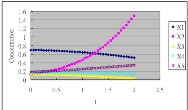
The chart of the basic time profile for the five genes can be depicted in Figure 1. First, we use equation (6) to estimate the derivatives at 40 time events:
39 , , 1 , 0 , 05 . ) 05 (. )) 1 ( 05 (. L = − + l l X l Xj j
Thus, each ODE in (8) is converted into a linear system of 40 equations. Each linear system is solved with the MLR package in
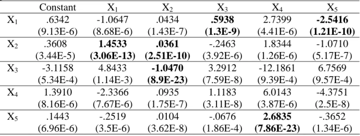
Excel with the estimated coefficients and p-values (in parentheses) reported in Table 2. Each row in the table represents the regression results of a linear system. The p-values of X3 and X5 on the first row are
several orders smaller than the p-values of other coefficients. Therefore, their corresponding coefficients are deemed significantly different from 0, compared to the other coefficients. According to the sign of the coefficients, we conclude that X3
activates X1 and X5 represses X1. The other
genes (X1, X2 and X4) have no regulatory
effects on the expression of X1. On the other
hand, if we choose the network coefficients based on the magnitude patterns as in [14], X4 would have a positive effect on X1. But,
this contradicts the network effects shown in Table 1, which lists the true coefficients corresponding to the LVS in (8). Following the same reasoning to track patterns of p-values for the other variables, we have bold-faced significant factors in the table. One can see that the p-value method has misrecognized the positive effect of X2 on
X2. However, since this coefficient (.0361)
is very small compared to the other coefficients, we may discard this network connection. The same method does not detect any significant pattern of p-values on the fourth row, though the regulating genes (X3 and X5) have the smallest p-values on
this row. Thus, the naïve conversion for this basic time profile has failed to detect the full network structure. 0 0.2 0.4 0.6 0.8 1 1.2 1.4 1.6 0 0.5 1 1.5 2 2.5 t C on cen tr at io n X1 X2 X3 X4 X5
Figure 1. Basic time profile of five genes
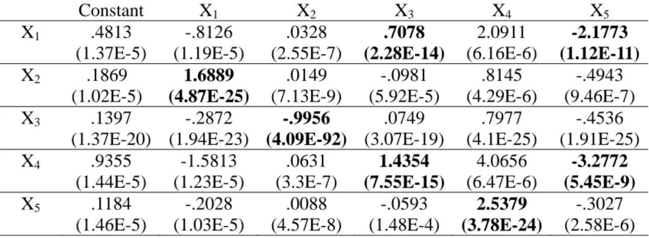
to convert LVS to linear systems, the regression results are reported in Table 3. One can see that, using the pattern detection of p-values, the network connections have been recognized correctly with signs according to the true values in Table 1. This shows the merits of the log conversion.
3.2 Using an expanded time profile
Since the default time gap of .05 provided by the basic time profile is too coarse to estimate the derivates, we expand the time profile by adding the RK4 outputs for every .01 change in the time domain. This has created an expanded profile of 201 events at 0, .01, .02, …, 1.99 and 2. The MLR results for the naïve and log conversions are respectively reported in Tables 4 and 5. One can observe two facts: first, the patterns of p-values can be more easily recognized; second, again the log conversion has provided more significant level with smaller p-value, and its estimated coefficients of significant genes are closer to the true values. This shows the merits of a finer time profile.
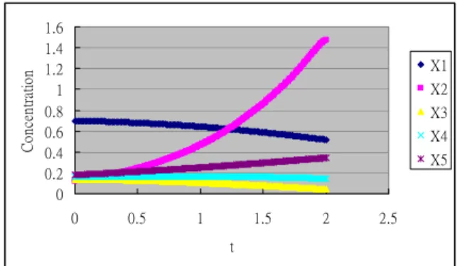
3.3 Expanded profile with cubic spline
Unfortunately, it is not always possible to expand the time profile by using RK4. Finding network coefficients is part of the job in a GRN problem. 0 0.2 0.4 0.6 0.8 1 1.2 1.4 1.6 0 0.5 1 1.5 2 2.5 t C onc en tr at io n X1 X2 X3 X4 X5
Figure 2. Expanded time profile with spline.
We use a cubic spline method to extend the basic time profile to an expanded profile
with the same fine resolution (.01) as above. This cubic spline matches a time trace at 41 time events: , l = 0, …, 40. Values of the spline at the step of .01 are plotted in Figure 2. The mean square errors between RK4 derived values and spline interpolated values of all five time traces are in the order of 1.0E-15. Using the spline expanded profile, we conduct the same experiments with the results reported in Table 6 (naïve conversion) and Table 7 (log conversion). These results are a little inferior to the results from the RK4 expanded profile. But, the pattern of p-values can still be easily recognized. Again, the log conversion provides better results than the naïve conversion. ) 05 (. l Xj 3.4 Using ANN
The basic profile is expanded with an ANN using the NeuroSolutions package from NeuroDimension, Inc. The network structure is 1 x 4 x 1, where 4 is the number of hidden nodes. A hyperbolic tangent (tanh) is selected as the activation function, and 50000 epochs of network training are conducted. The mean square errors between RK4 derived values and ANN predicted values for all five traces are in the order of 1.0E-6. The expanded time profile is plotted in Figure 3, which is again similar to Figure 1. However, the results for the log conversion, listed in Table 8, show several misidentified network connections.
0 0.2 0.4 0.6 0.8 1 1.2 1.4 1.6 0 0.5 1 1.5 2 2.5 t C onc en tr at io n X1 X2 X3 X4 X5
4. Conclusions
In this study, we model gene regulatory network by using a Lokta-Voltera system. A synthetic time profile of gene expressions is developed by solving the LVS with a RK4 algorithm. This time profile is used in a reverse engineering sense to derive the network coefficients of the LVS. We first convert the LVS into several independent systems of linear equations, which are solved with the MLR technique in statistics. Two conversions are used to estimate the derivatives in LVS: the naïve conversion and the log conversion. We use the pattern of p-values, which indicate the significant level of deviation from 0 for regression coefficients, to infer network coefficients. From the experiments, we conclude the following facts:
(1) Pattern detection of p-values can be used to infer network coefficients in LVS;
(2) The log conversion provides better results than the naïve conversion;
(3) When finer time profile is available, the results also improve; and
(4) The cubic spline method is better than the ANN method to expand a time profile in our case.
In the future, it pays to investigate why the ANN does not provide efficient and effective function approximation for the time profile. Are there other methods that can be used to better approximate the time profile? How is the p-value method affected by the noise commonly encountered in real gene expression profiles?
5. Acknowledgements
This research was supported in parts by
a grant from National Science Council (NSC) of Taiwan under the contract number NSC 94-2221-E-366-013. We are also grateful to the National Center for High-performance Computing (NCHC) for computer time and facilities.
6. References
[1] J.S. Almeida, E.O. Voit, “Neural-network-based parameter estimation in S-system models of biological networks”, Genome Informatics, vol. 14, pp. 114-123, 2003. [2] P. D’haeseleer, S. Liang, R. Somogyi,
“Genetic network inference: from co-expression clustering to reverse engineering”, Bioinformatics, vol. 16, pp. 707-726, 2000.
[3] M. Hirsch, S. Smale, differential equations, dynamical systems, and linear algebra, Academic Press, 1974.
[4] V.H. Hogg, E.A. Tannis, “Probability and Statistical Inference”, fifth edition, Prentice-Hall, 1997.
[5] P. Kennedy, “A Guide to Econometrics, fifth edition”, MIT Press, 2003.
[6] S. Kikuchi, D. Tominaga, M. Arita, K. Takahashi, M. Tomita, “Dynamic modeling of genetic networks using genetic algorithm and S-system”, Bioinformatics, vol. 19, pp. 643-650, 2003.
[7] H. Matsuno, A. Doi, M. Nagasaki, S. Miyano, “Hybrid Petri net representation of gene regulatory network”, Proceedings of pacific symposium on biocomputing, pp. 341-352, 2000.
[8] R. Mauricio, “Can ecology help genomics: the genome as ecosystem?”, Genetica, vol. 123, pp. 205-209, 2005. [9] N. Noman, H. Iba, “Revere engineering
genetic networks using evolutionary computation”, Genome informatics, vol. 16, pp. 205-214, 2005.
Bottani, J. Maller, F. d’Alche-Buc, “Gene networks inference using dynamic Bayesian networks”, Bioinformatics, vol. 19, pp. ii138-ii148, 2003.
[11] W. Press, B. Flannery, S. Teukolsky, W. Vetterling, “Numerical recipes in Fortran: The art of scientific computing”, 2nd ed. Cambridge, England, Cambridge University Press, 1992.
[12] J. Principe, N. Euliano, W. Lefebvre, “Neural and adaptive systems: fundamentals through simulations”, John Wiley & Sons, 1999.
[13] M.A. Savageau, E.O. Voit, “Recasting
nonlinear differential equations as S-systems: a canonical nonlinear form”, Mathematical Biosciences, vol. 87, pp. 83-115, 1987.
[14] S. Veflingstad, J. Almeida, E. Voit, “Priming nonlinear searches for pathway identification”, Theoretical biology and medical modeling, vol. 1, no. 8, pp. 1-14, 2004.
[15] E.O. Voit, M.A. Savageau, “Equivalence between S-systems and Volterra systems”, Mathematical Biosciences, vol. 78, pp. 47-55, 1986.
Table 1. True network coefficients.
Constant X1 X2 X3 X4 X5 X1 0 0 0 1 0 -1 X2 0 2 0 0 0 0 X3 0 0 -1 0 0 0 X4 0 0 0 2 0 -1 X5 0 0 0 0 2 0
Table 2. MLR estimated coefficients and p-values (in parentheses) with the basic time profile and naïve conversion.
Constant X1 X2 X3 X4 X5 X1 .6342 (9.13E-6) -1.0647 (8.68E-6) .0434 (1.43E-7) .5938 (1.3E-9) 2.7399 (4.41E-6) -2.5416 (1.21E-10) X2 .3608 (3.44E-5) 1.4533 (3.06E-13) .0361 (2.51E-10) -.2463 (3.92E-6) 1.8344 (1.26E-6) -1.0710 (5.17E-7) X3 -3.1158 (5.34E-4) 4.8433 (1.14E-3) -1.0470 (8.9E-23) 3.2912 (7.59E-8) -12.1861 (9.39E-4) 6.7569 (9.57E-4) X4 1.3910 (8.16E-6) -2.3366 (7.67E-6) .0935 (1.75E-7) 1.1183 (3.11E-8) 6.0143 (3.87E-6) -4.3751 (2.5E-8) X5 .1443 (6.96E-6) -.2519 (3.5E-6) .0104 (3.62E-8) -.0676 (1.86E-4) 2.6835 (7.86E-23) -.3652 (1.34E-6)
Table 3. MLR estimated coefficients and p-values (in parentheses) with the basic time profile and log conversion.
Constant X1 X2 X3 X4 X5 X1 .4813 (1.37E-5) -.8126 (1.19E-5) .0328 (2.55E-7) .7078 (2.28E-14) 2.0911 (6.16E-6) -2.1773 (1.12E-11) X2 .1869 (1.02E-5) 1.6889 (4.87E-25) .0149 (7.13E-9) -.0981 (5.92E-5) .8145 (4.29E-6) -.4943 (9.46E-7) X3 .1397 (1.37E-20) -.2872 (1.94E-23) -.9956 (4.09E-92) .0749 (3.07E-19) .7977 (4.1E-25) -.4536 (1.91E-25) X4 .9355 (1.44E-5) -1.5813 (1.23E-5) .0631 (3.3E-7) 1.4354 (7.55E-15) 4.0656 (6.47E-6) -3.2772 (5.45E-9) X5 .1184 (1.46E-5) -.2028 (1.03E-5) .0088 (4.57E-8) -.0593 (1.48E-4) 2.5379 (3.78E-24) -.3027 (2.58E-6)
Table 4. MLR estimated coefficients and p-values (in parentheses) with the expanded time profile and naïve conversion. Extra events come from RK4.
Constant X1 X2 X3 X4 X5 X1 .1210 (9.03E-18) -.2032 (7.14E-18) .0084 (1.19E-25) .9224 (9.8E-186) .5239 (3.89E-19) -1.2948 (2.0E-103) X2 .0630 (2.25E-15) 1.9058 (7.1E-206) .0065 (5.36E-39) -.0431 (2.79E-19) .3258 (1.16E-21) -.1906 (2.26E-23) X3 -.7462 (4.34E-11) 1.1725 (4.7E-10) -1.0170 (2.5E-216) .7525 (5.19E-25) -2.9705 (1.69E-10) 1.6482 (1.78E-10) X4 .2642 (5.67E-18) -.4440 (4.3E-18) .0179 (2.94E-25) 1.8324 (1.7E-178) 1.1451 (2.24E-19) -1.6427 (5.9E-65) X5 .0259 (1.65E-18) -.0453 (7.63E-20) .0019 (8.39E-29) -.0117 (2.26E-12) 2.1238 (4.1E-224) -.0659 (1.11E-21)
Table 5. MLR estimated coefficients and p-values (in parentheses) with the expanded time profile and log conversion. Extra events come from RK4.
Constant X1 X2 X3 X4 X5 X1 .0906 (4.64E-17) -.1530 (2.58E-17) .0062 (1.42E-24) .9450 (1.1E-209) .3946 (1.5E-18) -1.2223 (2.1E-119) X2 .0345 (8.79E-18) 1.9425 (8.0E-266) .0028 (4.31E-32) -.0179 (1.64E-14) .1510 (2.06E-19) -.0921 (2.55E-22) X3 .0221 (1.05E-59) -.0474 (2.39E-76) -.9996 (0) .0185 (1.57E-83) .1329 (1.36E-85) -.0758 (1.73E-87) X4 .1757 (5.47E-17) -.2972 (2.84E-17) .0120 (4.18E-24) 1.8940 (3.6E-212) .7657 (1.76E-18) -1.4290 (7.73E-81) X5 .0216 (4.14E-17) -.0371 (8.86E-18) .0016 (2.65E-28) -.0106 (6.99E-13) 2.0989 (1.0E-233) -.0557 (2.14E-20)
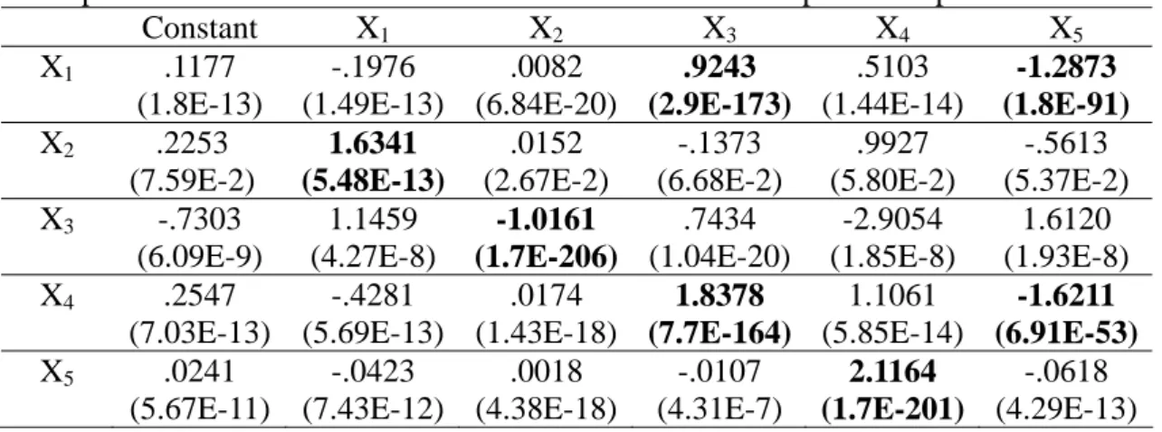
Table 6. MLR estimated coefficients and p-values (in parentheses) with the expanded time profile and naïve conversion. Extra events come from spline interpolation.
Constant X1 X2 X3 X4 X5 X1 .1177 (1.8E-13) -.1976 (1.49E-13) .0082 (6.84E-20) .9243 (2.9E-173) .5103 (1.44E-14) -1.2873 (1.8E-91) X2 .2253 (7.59E-2) 1.6341 (5.48E-13) .0152 (2.67E-2) -.1373 (6.68E-2) .9927 (5.80E-2) -.5613 (5.37E-2) X3 -.7303 (6.09E-9) 1.1459 (4.27E-8) -1.0161 (1.7E-206) .7434 (1.04E-20) -2.9054 (1.85E-8) 1.6120 (1.93E-8) X4 .2547 (7.03E-13) -.4281 (5.69E-13) .0174 (1.43E-18) 1.8378 (7.7E-164) 1.1061 (5.85E-14) -1.6211 (6.91E-53) X5 .0241 (5.67E-11) -.0423 (7.43E-12) .0018 (4.38E-18) -.0107 (4.31E-7) 2.1164 (1.7E-201) -.0618 (4.29E-13)
Table 7. MLR estimated coefficients and p-values (in parentheses) with the expanded time profile and log conversion. Extra events come from spline interpolation.
Constant X1 X2 X3 X4 X5 X1 .0872 (1.94E-11) -.1475 (1.28E-11) .0061 (6.06E-17) .9469 (2.2E-191) .3810 (1.65E-12) -1.2147 (1.0E-101) X2 .1947 (1.20E-1) 1.6745 (8.9E-14) .0114 (9.22E-2) -.1108 (1.33E-1) .8090 (1.17E-1) -.4579 (1.1E-1) X3 .0378 (4.03E-1) -.0737 (3.29E-1) -.9987 (2.3E-287) .0096 (7.19E-1) .1971 (2.90E-1) -.1115 (2.81E-1) X4 .1662 (8.0E-10) -.2813 (5.32E-10) .0115 (1.97E-14) 1.8993 (1.6E-187) .7269 (9.12E-11) -1.4074 (1.04E-59) X5 .0199 (4.52E-9) -.0341 (1.82E-9) .0015 (4.3E-16) -.0096 (1.13E-6) 2.0916 (2.3E-206) -.0516 (4.79E-11)
Table 8. MLR estimated coefficients and p-values (in parentheses) with the expanded time profile and log conversion. Extra events come from ANN approximation.
Constant X1 X2 X3 X4 X5 X1 19.7198 (1.22E-6) -36.5105 (1.63E-7) -.6664 (2.37E-4) 38.5948 (8.05E-19) 17.0428 (1.26E-1) -12.4503 (4.99E-2) X2 -54.6666 (6.48E-4) 102.2523 (1.94E-4) 7.2519 (9.32E-20) -196.2190 (1.09E-26) 127.0465 (4.69E-3) -52.0429 (4.08E-2) X3 104.4663 (4.38E-9) -193.0210 (2.81E-10) -4.2156 (1.26E-7) 191.701 (3.55E-23) 101.1365 (3.59E-2) -66.2539 (1.59E-2) X4 31.8514 (1.55E-9) -56.7898 (3.32E-10) .5310 (2.04E-2) 22.4063 (1.26E-5) 85.1122 (8.7E-9) -48.9753 (6.13E-9) X5 2.2575 (5.35E-1) -1.5745 (8.0E-1) 3.9801 (1.17E-60) -82.1367 (1.36E-56) 142.4317 (5.05E-31) -70.3187 (1.98E-25)