Pau-Lo Hsu, Member, IEEE
Abstract—Recently, modeling and simulation of hybrid dynamic systems (HDSs) have attracted much attention. However, since simulta-neously dealing with the discrete and continuous variables is very diffi-cult, most of the models result in a unified but more complicated and unnatural format. Moreover, design engineers cannot be allowed to use their preferred domain models. Based on the multiparadigm modeling concept, this correspondence proposes a Petri net framework with as-sociated state equations to model the HDSs. In the presented approach, modeling schemes of the hybrid systems are separated but combined in a hierarchical way through specified interfaces. Designers can still work in their familiar domain-specific modeling paradigms, and the heterogeneity is hidden when composing large systems. An application to a rapid thermal process in semiconductor manufacturing is provided to demonstrate the practicability of the developed approach.
Index Terms—Automated manufacturing systems, hybrid dynamic systems (HDSs), multiparadigm modeling (MPaM), Petri nets (PNs), semi-conductor manufacturing.
I. INTRODUCTION
One of the topics in critical reliability is the modeling and simu-lation of complex systems. In the past years, most work on system modeling and simulation has been mainly focused on either continuous variable systems (CVSs) or discrete-event systems (DESs). The former are typically modeled by differential or difference equations to analyze physical dynamic behavior, whereas the latter are described based on various frameworks to capture logical and sequential behaviors, such as finite-state automata, Petri nets (PNs), and max–min algebra [1]. As a paradigm, modeling is a way of representing our knowledge about the structure and behavior of systems to further answer questions about them. Both of the CVS and DES models are developed to reduce the complexity for presenting real systems. However, in practical applications, most systems possess the behavior that combines both the time-driven and event-driven dynamics together as the so-called hybrid dynamic systems (HDSs) or hybrid systems [2]–[4].
During the past decades, modeling and simulation of the HDS have attracted much attention. Integrating continuous and discrete models is
Manuscript received April 29, 2005; revised November 26, 2005 and June 19, 2006. This work was supported in part by the National Science Council, Taiwan, R.O.C., under Grant NSC 92-2917 I-009-005, by the Ministry of Education, Taiwan, R.O.C., under Grant Ex-91-E-FA06-4-4, by the Min-istry of Economic Affairs, Communication and Optoelectronics Infrastructure Construction Project, and Chang Jiang Scholars Program, PRC Ministry of Education. This paper was recommended by Associate Editor H. Pham.
J.-S. Lee is with the Information and Communications Research Laborato-ries, Industrial Technology Research Institute, Hsinchu 310, Taiwan, R.O.C. (e-mail: jinshyan_lee@itri.org.tw).
M. C. Zhou is with the Department of Electrical and Computer Engineering, New Jersey Institute of Technology, Newark, NJ 07102-1982 USA and also with School of Electro-Mechanical Engineering, Xidian University, Xi’an 710071, China (e-mail: zhou@njit.edu).
P.-L. Hsu is with the Department of Electrical and Computer Engineering, National Chiao-Tung University, Hsinchu 300, Taiwan, R.O.C. (e-mail: plhsu@ cc.nctu.edu.tw).
Color versions of one or more of the figures in this paper are available online at http://ieeexplore.ieee.org.
Digital Object Identifier 10.1109/TSMCA.2007.914747
part of a hybrid system in a collective PN model. Moreover, some commercial software has been developed, such as Simulink with the integration of Stateflow in the MATLAB platform [7] and VHDL-AMS/Verilog-AMS with the extensions of hardware description lan-guages to analog and mixed signals [8]. However, it is very difficult to simultaneously deal with the discrete and continuous variables. Their mathematical backgrounds are completely different: recurrence versus differential equations. Moreover, most of the existing approaches mix the continuous and discrete dynamics into a unified model, such as piecewise linear systems, hybrid PNs (HPNs) [9], and differential PNs. Hence, design engineers cannot be allowed to use their preferred domain models.
Over the years, different engineering domains have come up with various modeling abstractions that best suit the design of particular kinds of systems. Multiparadigm modeling (MPaM) is based on the premise of giving modelers the most appropriate modeling abstractions for their particular problem domain and integrating heterogeneous modeling techniques to achieve scalable designs. From an MPaM point of view, Lee and Hsu [10] extended the statechart of the unified modeling language to design a hybrid controller of automated vehicles and a three-axis motion control system [11] resulting in a clear and natural representation. Their proposed concept of the hybrid statechart is similar to the hybrid automata [12]. Generally speaking, either the statechart or automata mostly describes finite-state machines that are restricted to finite-state systems, whereas PN is better for present-ing infinite-state systems. Moreover, precise semantics and powerful analysis are required to prevent system deadlock and to discover the bottleneck in the present design [13]. PN provides powerful qualitative analysis and quantitative analysis, and also provides both rich visual formalism for specifying behavior and an executable notation [14]. Thus, based on the MPaM concept, this correspondence proposes a modeling approach within a PN framework. With different views of the system, it could be more efficient to work with separate inter-acting models. When composing large systems, designers can still work in their familiar domain-specific modeling paradigms so that the heterogeneity is hidden in this way. Moreover, resultant models are more natural than the HPN in [9] since the continuous part does not depend on a PN analogy to a continuous system, which is quite unnatural for continuous control systems. An example of a rapid thermal process (RTP) in semiconductor manufacturing is illustrated to show the feasibility of the proposed approach.
II. MPAMFORHYBRIDCONTROL A. Multiple Models in Hybrid Control
The art of system modeling is to choose the right level of abstraction to capture the aspects worth exploring, and to ignore the irrelevant details. This correspondence presents an MPaM approach within a PN-based framework for hybrid control systems. As shown in Fig. 1, a high-level coordination controller (within discrete-event domain) supervises the middle-level digital controller (within discrete-time domain) through two interfaces: signal generator and event generator. The signal generator is applied to transform the action commands
Fig. 1. Multiple domains in hybrid control systems.
from the coordination controller to digital signals, whereas the event generator is used to trigger events according to some critical thresholds in digital signals. Then, the digital controller regulates the low-level physical plant (within a continuous-time domain) via two interfacing devices: sampler and holder. The sampler is used to generate the digital signals by sampling the analog signals in the physical plant, whereas the holder is applied to construct the piecewise-continuous analog signals. Note that signal or event conversions through boundary interfaces could be multiple signals or events with a vector or matrix format. In practice, a coordination controller supervises more than one digital device of physical plant, particularly in the fields of logical control for an automated manufacturing system, traffic control of a highway, and sequence control of a chemical process. Fig. 1 also shows a typical centralized and hierarchical control scheme, in which the coordination controller supervises several digital controllers in a hierarchical way.
In the presented approach, the discrete-event, discrete-time, and continuous-time models are connected together in a hierarchical way to form the whole systems. Even though the proposed model presen-tation is more compact and simpler in a natural way, it is noted that conjunct interfaces of heterogeneous models are an important issue. In this correspondence, the interfacing devices for the communication among models have been described.
B. PN Framework for Discrete-Event and Discrete-Time Domains
From the MPaM point of view, in the discrete-event domain, the PN is employed to model and design the coordination controller. The main motivation for using PN as hybrid models is the fact that all those good features that make discrete PN a valuable discrete-event model are still available to hybrid systems. Examples of these features are as follows: PN does not require the exhaustive enumeration of the state space and can finitely describe systems with an infinite-state space. In addition, PN allows modular representation where the structure of each module is kept in the composed model. Moreover, the discrete state of PN is represented by a vector and not by a symbolic label; thus, linear algebraic techniques may be used for analysis.
Fig. 2 shows the proposed PN framework for modeling the discrete-event and discrete-time domains. Each operation is modeled with a command transition to start the operation, a progressive working place, a response transition to end the operation, and a completed place. Note that the start transition (drawn with a dark symbol) is a controllable event as “command” input, whereas the end transition is an uncontrollable event as “response” output. The working place is a hierarchical hybrid place (HHP, drawn with a triple circle), in which the state equations under controlled systems are contained and interacted through the boundary interface. The interaction between the event-driven and time-driven domains is achieved in the following way: a token put into the working place starts the integration of the
Fig. 2. Modeling the continuous dynamics within a PN via a hierarchical way.
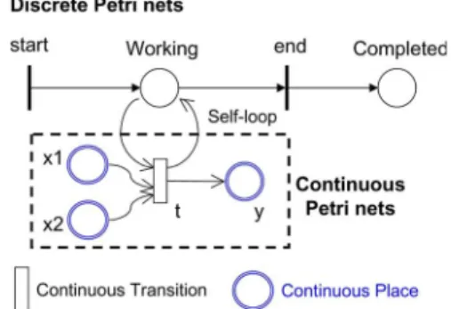
Fig. 3. HPN (with a net structure to model continuous dynamics).
corresponding equations. Concurrently with the integration, a certain number of thresholds are monitored. Each threshold is associated with a transition, i.e., the response transitions. When the threshold is crossed, it means that the corresponding event is occurring and that the attached transition is fired. The new marking is computed, and the integration of a new system starts.
C. State Equations for Discrete-Time and Continuous-Time Domains
On the other hand, in the hybrid subsystem of discrete-time and continuous-time domains, i.e., the so-called sampled-data system, differential and difference equations or Laplace S and Z functions are typically used to model and analyze such systems. This correspon-dence is focused on the modeling of the hybrid system from the high-level viewpoint. Design approaches of the coordination and digital controllers will be briefly mentioned in the following sections. D. Comparison With Other Modeling
HPN [9] contains both conventional discrete PN and continuous PN, as shown in Fig. 3. In this model, the discrete part is represented by the discrete places and transitions, and the continuous part is by the continuous places (drawn with a double circle) and transitions. In the continuous PN, the marking of a place is a real positive number, and the firing is carried out like a continuous flow. The unique way of describing interactions between the continuous part and the discrete one is by means of self-loops. Basically, the discrete PN is applied to trigger the continuous transitions. However, this approach can only describe real and nonnegative continuous variables. Moreover, a continuous place represents only one continuous variable, e.g., the x1, x2, and y in Fig. 3. In basic HPN, only continuous variables that are linear with respect to time could be represented as constant speeds. It has been extended to represent other kinds of evolutions, but for each kind of evolution, a new type of continuous place has to be introduced. In this correspondence, instead of using the net structure (i.e., the continuous PN in HPN) to model the continuous part of the system, the proposed framework, which is shown in Fig. 2, uses
Fig. 4. Interfacing devices in high level. (a) Signal and (b) event generators.
the original state equations to represent the continuous system dy-namics. In this way, it can be said that the PN (event-driven part of the model) coordinates the system of difference-algebraic equations whose structure changes each time a transition is fired. Also, the system of equations (time-driven part of the model) regulates the PN evolutions by enforcing the firing of its transition via the threshold-crossing mechanism. The proposed approach allows the use of the domain-specific primitive models, such as differential/difference equa-tions, to capture low-level physical interactions and then be connected with the high-level PN in a hierarchical way. Thus, the resultant model with a natural description is more compact and simpler than HPN. Although the framework we are presenting is general in nature, in this correspondence, we will concentrate on the specific class of semiconductor manufacturing systems that largely motivate this work. Moreover, as compared with the sequential function chart (SFC), modeling the discrete-event flow and distributing the continuous part to embedded controllers that report back their state to the event-driven logic controllers, the proposed approach based on a PN frame-work is more formal. The SFC is derived from PN with some simplifications; therefore, theoretical results of PN cannot be directly applied to SFC [15]. In our PN framework, a formal analysis of some important properties, including boundness (no capacity overflow), liveness (freedom from deadlock), conservativeness (conservation of nonconsumable resources), and reversibility (cyclic behavior), could be easily performed. Their validation methods include reachability analysis, invariant analysis, reduction method, siphons/traps-based approach, or simulation [14].
III. DISCRETE-EVENT ANDDISCRETE-TIMEMODELS
The upper part in Fig. 1 shows a typical hybrid structure of the discrete-event and discrete-time models. In this section, we briefly review the DESs and then describe the interfaces and controller design of such hybrid systems.
A. DESs
A DES is a dynamic asynchronous system, where the state transi-tions are initiated by events that occur at discrete instants of time. The state of a DES may change abruptly at the occurrence of an event, and in between two events, the system remains in the same state.
B. Interfaces Between Discrete-Event and Discrete-Time Models
Signals in discrete-event and discrete-time models are fundamen-tally different. When combining these models, appropriate signal conversion mechanisms need to be introduced. Most signal conver-sion algorithms are application-specific and must be implemented as separate components. As shown in Fig. 4(a), a signal generator is a device that converts a discrete event into a digital signal. This device typically uses an event as the input command (such as to push a button)
In this correspondence, we directly adopt the supervisor synthesis method from the study in [16] to build the PN model of the coordina-tion controller. The design procedure consists of the following steps.
Step 1) Construct the PN model of the plant.
Step 2) Construct the PN model of the specifications (e.g., the sequence of processes, operation switching, and resource constraints).
Step 3) Compose the plant and specification models to yield the coordination controller.
Step 4) Verify and refine the coordination controller to obtain a live bounded and reversible model.
In this present scheme, the designer of coordination controllers can purely focus on the discrete-event and discrete-time domains without considering the detailed complex dynamics of the low-level physical systems.
IV. DISCRETE-TIME ANDCONTINUOUS-TIMEMODELS
The lower part in Fig. 1 shows a typical hybrid configuration of the continuous-time plant with a discrete-time feedback controller, i.e., the so-called sampled-data system. In this section, we briefly review such a kind of system and discuss its controller design for hybrid systems.
A. Sampled-Data Systems
A sampled-data system combines both continuous- and discrete-time dynamic subsystems. Because of this inherent mixture of discrete-time domains, we shall also refer to a sampled-data system as a hybrid system. Although the plant is usually a continuous-time (or analog) system, in most practical applications, the controller is a discrete-time (or digital) device. This is mainly due to the numerous advantages that digital equipment offers over their analog counterparts. With the great advances in computer technology, today, digital controllers are more compact, reliable, flexible, and often less expensive than analog ones.
B. Interfaces Between Discrete-Time and Continuous-Time Models
There is a fundamental operational difference between digital and analog controllers, i.e., the digital system acts on samples of the measured plant output rather than on the continuous-time signal. A practical implication of this difference is that a digital controller requires special interfaces that link it to the analog world.
A digital controller (i.e., a discrete-time controller) can be idealized as one with three main elements: the analog-to-digital (A/D) interface, digital computer, and digital-to-analog (D/A) interface. As shown in Fig. 5(a), the A/D interface or sampler acts on a physical variable, normally an electric voltage, and converts it into a sequence of binary numbers, which represent the values of the variable at the sampling instants. These numbers are then processed by the digital computer, which generates a new sequence of binary numbers that correspond to the discrete control signal. As shown in Fig. 5(b), this control signal is finally converted into an analog voltage by the D/A interface, also called the holder. The digital computer implements the control
Fig. 5. Interfacing devices in low level. (a) Sampler and (b) holder.
algorithm as a set of difference equations, which represent a dynamic system in the discrete-time domain.
C. Digital Controller Design
Basically, two classic approaches are taken in continuous-time and discrete-time domains, respectively, for a digital controller design. The first technique, which is referred to as emulation [17], is the most widely applied in industries. Emulation consists in first designing an analog controller such that the closed-loop system has satisfactory properties and then translating the analog design into a discrete one using a suitable discretization method. This technique has the advan-tage that the synthesis is done in continuous time, where the design goals are typically specified and where most of the designer’s experi-ence and intuition reside. In addition, the system’s analog performance will, in general, be recovered for fast sampling. The second traditional technique consists in discretizing the plant and performing a controller design in the discrete-time domain directly. The main benefit of this approach is that the synthesis procedure is again simplified since the discretized plant is linear time-invariant in the discrete-time domain. In this presented MPaM scheme, both approaches are acceptable. Thus, the designers of digital controllers can easily focus on the discrete-time and continuous-discrete-time domains and use their preferable approaches without considering the logical behaviors of the high-level system.
V. APPLICATIONEXAMPLE
This section demonstrates a practical application of the hybrid control for an RTP. The status of the hybrid RTP system at any time instant involves the upper event-driven states and lower time-driven states of all components in the system at that time.
A. Description of the RTP System
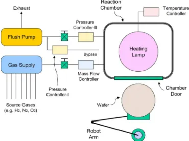
An RTP is a relatively new semiconductor manufacturing device [18]. A schematic diagram of the RTP system is shown in Fig. 6, which is composed of: 1) a reaction chamber with a door; 2) a robot arm for wafer loading/unloading; 3) a gas supply module with a mass flow controller and pressure controller-I; 4) a heating lamp module with a temperature controller; and 5) a flush pumping system with a pressure controller-II. Note that the initial state of the components in the RTP is either closed or off, except that the door is open. A realistic “recipe” of the hydrogen baking process is as follows.
Step 1) Load the raw wafer. Step 2) Close the chamber door.
Step 3) Open the gas valve to supply gases with a desired gas flow rate and pressure of 2.8 L/min (l pm) and 0.55 torr., respectively.
Step 4) Close the gas valve.
Step 5) Turn on the heating lamp to bake the wafer with a desired baking temperature and duration of 1000 ◦C and 4 s, respectively.
Fig. 6. Schematic diagram of the RTP system.
Step 6) Turn off the heating lamp to cool down the chamber to a desired temperature of less than 20◦C.
Step 7) Turn on the flush pump with a desired pressure of less than 0.05 torr.
Step 8) Turn off the flush pump. Step 9) Open the chamber door. Step 10) Unload the processed wafer. B. System Modeling and Simulation
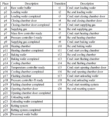
By applying the design procedure in Section III-C, the PN model of RTP is constructed as shown in Fig. 7, which consists of 26 places and 20 transitions, respectively. Corresponding notations are described in Table I. After constructing the PN model, we can perform the model validation of the dynamic behavior. Due to its graphical representation, ease of manipulation, and ability to perform structural analysis, the software package ARP [19] is adopted to verify the behavioral properties of the developed PN model. Validation results reveal that the present PN model is live and bounded.
By interacting with the time-driven dynamics, Fig. 8 shows the pressure and temperature of one cycle (assume linear variation) for a wafer processing in RTP, including the wafer loading, door closing, gas supplying, chamber heating, wafer baking, chamber cooling, chamber flushing, door opening, wafer unloading, and system resetting. In Fig. 8(a), the controlled event t5 (start supplying gas) occurs at about the 4th second and enables the HHP p6 for supplying gas. Then, t7 (start heating chamber) happens at about the 13th second, as shown in Fig. 8(b), and makes the HHP p10 for heating the chamber. After t9 (start baking wafer) occurs at about the 19th second, the wafer is baking at HHP p12. For the period 19th to 23rd seconds, it could be a PID steady state control of temperature at 1000◦C for 4 s. After baking, t11 (start cooling chamber) happens to locate the token in HHP p14 for cooling the chamber. At about the 36th second, t13 (start flushing chamber) occurs to flush the chamber at HHP p17. Then, t15 (start opening chamber door) happens at the 53rd second to further the followed wafer unloading. This simulation result indicates that the corresponding discrete events are successfully triggered according to the desired crossing thresholds of the continuous variables in the time domain.
VI. CONCLUSION
This correspondence presents an MPaM approach within a PN framework for HDSs. The presented approach allows the use of
Fig. 7. PN model of the RTP system.
TABLE I
NOTATION FOR THEPNOF THERTPINFIG. 7
preferred domain models and leads to a more natural representation of the continuous part using a hierarchical framework. Designers can still work in their familiar domain-specific modeling paradigms, and the heterogeneity is hidden when composing large systems. Multiple models can then be hierarchically composed to build complex models. Thus, through combining the use of well-established theories of PN and differential/difference equations, each one being well suited for an aspect of the problem, we emphasize on the interface between the aspects.
Fig. 8. (a) Pressure and (b) temperature in the RTP system for one-cycle processing.
In this correspondence, the interactions between discrete events and continuous variables are transformed based on interfaces as described in Sections III-B and IV-B, and some special conditions should be further discussed, such as multiple threshold value crossings. Also, a variable may be treated as either a discrete or continuous one depend-ing on different operational contexts at different times. Basically, in the operational context of the discrete-event domain, the coordination con-troller treats the variable as a discrete state, whereas in the context of the discrete-time domain, the digital controller handles the variable as
a dynamic state. For example, the coordination controller manipulates a discrete-state “heating chamber” in the RTP application, whereas the digital controller regulates the continuous-state “temperature” dynamically with regard to the implemented recipe. Future research includes the application of the MPaM approaches to various industrial systems that are of complex discrete-event and continuous dynamics and must meet economical, environmental, and life-cycle engineering requirements [20]–[25].
REFERENCES
[1] C. G. Cassandras and S. Lafortune, Introduction to Discrete Event
Systems. Boston, MA: Kluwer, 1999.
[2] A. S. Morse, C. C. Pantelides, S. S. Sastry, and J. M. Schumacher, “Introduction to the special issue on hybrid systems,” Automatica, vol. 35, no. 3, pp. 347–348, Mar. 1999.
[3] P. J. Antsaklis and M. D. Lemmon, “Introduction to the special issue,” J. Discrete Event Dynamic Syst., vol. 8, no. 2, pp. 101–103, Jun. 1998.
[4] P. J. Antsaklis and A. Nerode, “Hybrid control systems: An introductory discussion to the special issue,” IEEE Trans. Autom. Control, vol. 43, no. 4, pp. 457–460, Apr. 1998.
[5] J. Liu and E. A. Lee, “A component-based approach to modeling and sim-ulating mixed-signal and hybrid systems,” ACM Trans. Model. Comput.
Simul., vol. 12, no. 4, pp. 343–368, Oct. 2002.
[6] I. Demongodin and N. T. Koussoulas, “Differential Petri nets: Represent-ing continuous systems in a discrete-event world,” IEEE Trans. Autom.
Control, vol. 43, no. 4, pp. 573–578, Apr. 1998.
[7] T. Harman and J. Dabney, Mastering Simulink 4. Englewood Cliffs, NJ: Prentice-Hall, 2001.
[8] K. Bakalar and E. Christen, “VHDL 1076.1: Analog and mixed signal extensions for VHDL,” IEEE, Piscataway, NJ, Tech. Rep., 1999. [9] R. David and H. Alla, “Petri nets for modeling of dynamics systems—
A survey,” Automatica, vol. 30, no. 2, pp. 175–202, 1994.
[10] J. S. Lee and P. L. Hsu, “Statechart-based representation of hybrid con-trollers for vehicle automation,” Proc. Inst. Electr. Eng.—Intell. Transp.
Syst., vol. 153, no. 4, pp. 253–258, Dec. 2006.
[11] J. S. Lee and P. L. Hsu, “UML-based modeling and multi-threaded sim-ulation for hybrid dynamic systems,” in Proc. IEEE Int. Conf. Control
Appl., Glasgow, U.K., Sep. 2002, pp. 1207–1212.
[12] J. Lygeros, K. H. Johansson, S. N. Simic, J. Zhang, and S. S. Sastry, “Dynamical properties of hybrid automata,” IEEE Trans. Autom. Control, vol. 48, no. 1, pp. 2–17, Jan. 2003.
[13] J. S. Lee and P. L. Hsu, “Design and implementation of the SNMP agents for remote monitoring and control via UML and Petri nets,” IEEE Trans.
Control Syst. Technol., vol. 12, no. 2, pp. 293–302, Mar. 2004.
[14] M. C. Zhou and M. D. Jeng, “Modeling, analysis, simulation, schedul-ing, and control of semiconductor manufacturing systems: A Petri net approach,” IEEE Trans. Semicond. Manuf., vol. 11, no. 3, pp. 333–357, Aug. 1998.
[15] I. Miyazawa, H. Tanaka, and T. Sekiguchi, “Verification of the behavior of sequential function chart based on its Petri net model,” in Proc. IEEE
Int. Conf. ETFA, Sep. 1997, pp. 532–537.
[16] J. S. Lee and P. L. Hsu, “Remote supervisory control of the human-in-the-loop system by using Petri nets and Java,” IEEE Trans. Ind. Electron., vol. 50, no. 3, pp. 431–439, Jun. 2003.
[17] G. Franklin, J. Powell, and M. Workman, Digital Control of Dynamic
Systems. Reading, MA: Addison-Wesley, 1990.
[18] R. B. Fair, Rapid Thermal Processing: Science and Technology. New York: Academic, 1993.
[19] C. A. Maziero, “ARP: Petri net analyzer,” in Control and
Microinfor-matic Laboratory. Santa Catarina, Brazil: Federal Univ. Santa Catarina,
1990.
[20] N. Wu and M. C. Zhou, “Resource-oriented Petri net for deadlock avoid-ance in flexible assembly systems,” IEEE Trans. Syst., Man, Cybern. A,
Syst., Humans, vol. 38, no. 1, pp. 56–69, Jan. 2008.
[21] Y. Du, C. Jiang, and M. C. Zhou, “Modeling and analysis of real-time cooperative systems using Petri nets,” IEEE Trans. Syst., Man, Cybern. A,
Syst., Humans, vol. 37, no. 5, pp. 643–654, Sep. 2007.
[22] Z. W. Li, H. S. Hu, and A. R. Wang, “Design of liveness-enforcing supervisors for flexible manufacturing systems using Petri nets,” IEEE
Trans. Syst., Man, Cybern. C, Appl. Rev., vol. 37, no. 4, pp. 517–526,
Jul. 2007.
[23] N. Wu, L. Bai, and C. Chu, “Modeling and conflict detection of crude oil operations for refinery process based on controlled colored timed Petri net,” IEEE Trans. Syst., Man, Cybern. C, Appl. Rev., vol. 37, no. 4, pp. 461–472, Jul. 2007.
[24] P. Yan and M. C. Zhou, “A life-cycle engineering approach to develop-ment of flexible manufacturing systems,” IEEE Trans. Robot. Autom., vol. 19, no. 3, pp. 465–473, Jun. 2003.
[25] M. C. Zhou, F. DiCesare, and D. Rudolph, “Design and implementation of a Petri net based supervisor for a flexible manufacturing system,”