IEEE 802.16e OFDMA 下行通道估測技術之探討與數位訊號處理器實現

國

立

交

通

大

學

電子工程學系 電子研究所碩士班

碩

士

論

文

IEEE 802.16e OFDMA 下行通道估測技術之探討與

數位訊號處理器實現

Research in and DSP Implementation of Channel

Estimation Techniques for IEEE 802.16e OFDMA

Downlink

研 究 生：王 智 維

指導教授：桑 梓 賢 教授

IEEE 802.16e OFDMA 下行通道估測技術之探討與數位訊號處

理器實現

Research in and DSP Implementation of Channel Estimation

Techniques for IEEE 802.16e OFDMA Downlink

研 究 生：王智維 Student：Chih-Wei Wang

指導教授：桑梓賢 教授 Advisor：Tzu-Hsien Sang

國 立 交 通 大 學

電子工程學系 電子研究所碩士班

碩 士 論 文

A Thesis

Submitted to College of Electrical and Computer Engineering National Chiao Tung University

in partial Fulfillment of the Requirements for the Degree of

Master in

Electronics Engineering January 2008

Hsinchu, Taiwan, Republic of China

中 華 民 國 九 十 七 年 一 月

IEEE 802.16e OFDMA 下行通道估測技術之探討與數位

訊號處理器實現

研究生：王智維 指導教授：桑梓賢 教授

國立交通大學

電子工程研究所碩士班

摘要

正交分頻多工(OFDM)技術已經成功地被應用在普遍數位通訊的應用中。採 用 OFDM 的主要原因之一是可抵抗對於多重路徑干擾的效應。我們著重在 IEEE 802.16e OFDMA 下行的通道估測部分，且用數位訊號處理器去實現通道估測的機 制。此數位訊號處理器的環境是Freescale Semiconductor 的 MSC8126ADS，是個 擁有四個運算核心的多工處理器。 我們探討了三種通道估測的方法，一個是二維的線性內插，一個是二維的非 線性內插，另一個是最小平方法(Least-squares)。在通道被前面兩種方法估測出來 後，我們用最小平均平方誤差等化器的方法去減少在移動的環境所造成的載波間 互相干擾(ICI)。我們分別在靜態及時變的 Rayleigh 通道上驗證我們的模擬模型。 至於數位訊號處理器的部分，在運算復雜度與效能之間的做最有利益的選 擇，所以只採用簡單的二維線性內插法，可以達到很好的速度之外，也有可以接 受的結果。為了增加執行的速度，我們將寫定點數運算的C 程式去應用在數位訊

Research in and DSP Implementation of Channel

Estimation Techniques for IEEE 802.16e OFDMA

Downlink

Student：Chih-Wei Wang Advisor：Tzu-Hsien Sang

Department of Electronics Engineering & Institute of Electronics

National Chiao Tung University

ABSTRACT

Orthogonal frequency division multiplexing (OFDM) has been successfully applied to a wide variety of digital communications applications over the past several years. One of the main reasons to use OFDM is its robustness when facing channel multi-path dispersion. We focus on the OFDMA downlink channel estimation with a reference framework of IEEE 802.16e. Also, we implemented OFDMA downlink channel estimation schemes on a digital signal processor. The DSP is a Freescale Semiconductor’ MSC8126ADS, which is a four-core signal processor.

We study three channel estimation methods; two are based on two-dimensional linear and non-linear interpolations, then another is formulated as a least squares problem. After channels are estimated by aforementioned methods, we used a block MMSE equalizer to reduce inter-carrier interference in mobile environment. We verify the performance with numerical simulations on both static and time-variant fading

channels.

As for the DSP implementation, a two-dimensional linear interpolation is chosen due to its computational complexity. The DSP implementation is also carried out with fixed point formats.

誌 謝

首先感謝恩師 桑梓賢教授在交通大學研究所求學兩年半的細心指導，對於我 的研究方向給予很多的建議讓我可以順利完成這篇論文. 同時也感謝欣徳學長在 我念研究所之中的協助, 一些經驗的傳承給予我很大的收穫.當然也要感謝實驗室 的同學們,在有問題時可以與你們討論找出自己的盲點, 很高興認識你們. 最後,感謝我的父母,無怨無悔的給予我生活上的精神上的支持,以及女友郭小 柔在我苦惱的時候也在旁鼓勵我,總之感謝各位.

Contents

Chapter 1 Introduction to IEEE 802.16e OFDMA Physical Layer... 1

1.1 Overview of OFDM and OFDMA Systems... 1

1.2 Overview of Mobile WiMAX ... 4

1.3 Overview of IEEE 802.16e Downlink ... 4

1.3.1 OFDMA Frame Structure ... 5

1.3.2 Modulation... 7

1.3.3 Sub-carrier Allocation ... 8

Chapter 2 The DSP Hardware and Associated Software Development Environment ... 14

2.1 The MSC8126ADS board ... 14

2.1.1 MSC8126ADS Board Features ... 14

2.1.2 MSC8126 Features ... 16

2.2 Developing Optimized Code for Speed on the SC140 Cores... 20

2.2.1 Loop unrolling ... 20

2.2.2 Split Computation ... 21

2.2.3 Multisampling... 22

Chapter 3 Channel Estimation Techniques for IEEE 802.16e Downlink and DSP Implementation ... 25

3.1.1 Channel estimation with linear interpolation (LI) ... 26

3.1.2 Channel Estimation with circular interpolation (CI) ... 28

3.1.3 Least-Square (LS) Estimator with time-domain linear interpolation ... 29

3.1.4 ICI Cancellation by Equalization of Time-Varying Channels 31 3.1.5 Computational Complexity Analysis ... 32

3.2 Simulation Channel Model and OFDMA Downlink System Parameters ... 32

3.3 Performance of Channel Estimation ... 35

3.3.1 Simulation Flows ... 35

3.3.2 Floating-point Simulation... 36

3.4 DSP Implementation ... 43

3.4.1 Implementation of Transmitter... 43

3.4.2 Implementation of Receiver at channel estimation... 48

3.5 WiMAX System Integration on the DSP Platform ... 51

Chapter 4 Conclusions and Future Work ... 53

4.1 Conclusions ... 53

4.2 Future Work ... 54

List of Figures

Fig. 1.1 Basic architecture of an OFDM system [3]... 3

Fig. 1.2 Insertion of CP [3]. ... 3

Fig. 1.3 OFDMA sub-carriers. ... 3

Fig. 1.4 Mobile WiMAX system profile. ... 4

Fig. 1.5 OFDMA frequency description (3-channel schematic example) [4].. 5

Fig. 1.6 Example of an OFDMA frame (with only mandatory zone) in TDD mode [5]... 6

Fig. 1.7 Downlink basic structure [4]. ... 9

Fig. 1.8 Cluster structure [3]... 10

Fig. 2.1 MSC8122/8126ADS Top-side Part Location Diagram [6]... 15

Fig. 2.2 MSC8126 Block Diagram [7]. ... 18

Fig. 2.3 SC140 Extended Core Block Diagram [7]. ... 19

Fig. 3.1 Cluster structure [9]... 26

Fig. 3.2 Pilot distribution in successive clusters [9]. ... 27

Fig. 3.3 Block diagram of the simulated system... 35

Fig. 3.4 The comparison of different SUI-3 channel estimated methods in performance (Using Preamble)... 37

Fig. 3.5 The comparison of different SUI-3 channel estimated methods in performance. (a) MSE. (b) BER. ... 38

Fig. 3.6 The comparison of channel frequency responses which are

estimated by different algorithms... 39

Fig. 3.7 BER performance of different algorithms with various velocities and CFO = 0.02 × tone spacing frequency. ... 39

Fig. 3.8 Average cluster BER performance in SUI-3 at 30 dB SNR. (a) Odd symbol. (b) Even symbol... 40

Fig. 3.9 Average cluster MSE performance in SUI-3 at 30 dB SNR. (a) Odd symbol. (b) Even symbol... 41

Fig. 3.10 Performance of ICI cancellation algorithm with various velocities.42 Fig. 3.11 Performance of ICI cancellation algorithm with various velocities & CFO = 0.02 × tone spacing frequency... 42

Fig. 3.12 DL UP and FP chain on MSC8126. ... 43

Fig. 3.13 DL processing functions... 45

Fig. 3.15 Histogram of UP function cycle count... 47

Fig. 3.16 Histogram of FP function cycle count. ... 48

Fig. 3.17 Simulation system. ... 48

Fig. 3.18 Performance of comparison between floating-point and fixed-point computation in SUI-3 for various Doppler frequencies with preamble. ... 49

Fig. 3.19 Performance of comparison between floating-point and fixed-point computation in SUI-3 for various Doppler frequencies. (a) BER. (b) MSE.50 Fig. 3.20 Histogram of Channel Estimation function cycle count... 51

List of Tables

Table 1.1 OFDMA DL-PUSC Sub-carrier Allocations... 10

Table 2.1 MSC8126 ADS board features ... 16

Table 2.2 MSC8126 Features ... 17

Table 3.1 Computational Complexity ... 32

Table 3.2 OFDMA Downlink Parameters ... 34

Table 3.3 Terrain Type vs. SUI Channels ... 34

Table 3.4 General Characteristic of SUI Channels... 34

Table 3.5 SUI-3 Channel Model ... 35

Table 3.6 Cycle Count of DL UP ... 46

Table 3.7 Cycle Count of DL FP ... 47

Table 3.8 Cycle Count of Channel Estimation ... 51

Table 3.9 Throughput of WiMAX 16e Transmitter on MSC8126... 52

Chapter 1 Introduction to IEEE

802.16e OFDMA Physical Layer

IEEE 802.16 has developed the IEEE Standard 802.16-2004 for broadband wireless access systems, which provides a variety of services to fixed outdoor as well as nomadic indoor users. The mobile extension, referred to as 802.16e, can support new capabilities needed for the mobile environment. The object of this thesis focuses on the downlink channel estimation part for WirelessMAN-OFDM and WirelessMAN-OFDMA.

This chapter is organized as follows. In section 1.1 and section 1.2, we gave the overview of OFDMA systems and mobile WiMAX systems respectively. In section 1.3, we described OFDMA downlink specifications in IEEE 802.16e briefly.

1.1 Overview of OFDM and OFDMA Systems

According to [1] and [2], orthogonal frequency division multiplexing (OFDM) is a multiplexing technique that divides the bandwidth into multiple frequency sub-carriers as shown in Fig. 1.1. The input data stream of an OFDM system is subdivided into several parallel sub-streams of reduced data rate (thus increased symbol duration) and each sub-stream is modulated and transmitted on a separate orthogonal sub-carrier. The increased symbol duration improves the robustness of

OFDM to channel delay spread. OFDM converts a frequency-selective channel into a parallel collection of frequency flat sub-channels.

The sub-carriers have the minimum frequency separation required to maintain orthogonality of their corresponding time domain waveforms, yet the signal spectra corresponding to the different sub-carriers overlap in frequency. Hence, the available bandwidth is used very efficiently. Furthermore, the introduction of the cyclic prefix (CP) shown in Fig. 1.2 can completely eliminate inter-symbol interference (ISI) as long as the CP duration is longer than the channel delay spread. OFDM modulation can be realized with efficient IFFT, which enables a large number of sub-carriers (up to 2048) with low complexity.

In an OFDM system, resources are available in the time domain by means of OFDM symbols and in the frequency domain by means of sub-carriers. The time and frequency resources can be organized into sub-channels for allocation to individual users. Orthogonal frequency division multiple access (OFDMA) in [4] and [5] is a multiple-access/multiplexing scheme that provides multiplexing operation of data streams from multiple users onto the downlink sub-channels and uplink multiple access is achieved by assigning subsets of sub-carriers to individual users as shown in Fig. 1.3. This allows simultaneous low data rate transmission from several users. Different number of sub-carriers can be assigned to different users, in view to support differentiated quality of service (QoS), i.e. to control the data rate and error probability individually for each user.

Fig. 1.1 Basic architecture of an OFDM system [3].

Fig. 1.2 Insertion of CP [3].

1.2 Overview of Mobile WiMAX

The WiMAX technology, based on the IEEE 802.16-2004 air interface standard [4] is rapidly proving itself as a technology that will play a key role in fixed broadband wireless metropolitan area networks. Mobile WiMAX that adopts OFDMA for improved multi-path performance in non-line-of-sight environments is a broadband wireless solution that enables convergence of mobile and fixed broadband networks through a common wide area broadband radio access technology and flexible network architecture. It offer scalability in both radio access technology and network architecture, thus providing a great deal of flexibility in network deployment options and service offerings. Scalable OFDMA (SOFDMA) is introduced in the IEEE 802.16e standard [5] amendment to support scalable channel bandwidths from 1.25 to 20 MHz. Release-1 mobile WiMAX profiles that is completed in early 2006 (see Fig. 1.4 from [3]) will cover 5, 7, 8.75, and 10 MHz channel bandwidths for licensed worldwide spectrum allocations in the 2.3 GHz, 2.5 GHz, 3.3 GHz and 3.5 GHz frequency bands.

Fig. 1.4 Mobile WiMAX system profile.

In OFDMA, the active sub-carriers are divided into subsets of sub-carriers where each subset is termed a sub-channel. The sub-carriers forming one sub-channel may, but need not be, adjacent. Fig. 1.5 can describe clearly the concept.

Three basic types sub-channel organization are defined in [4] and [5]: partial usage of sub-channels (PUSC), full usage of sub-channels (FUSC), and adaptive modulation and coding (AMC) among which the PUSC is mandatory and the other two are optional. In PUSC DL, the entire channel bandwidth is divided into three segments to be used separately. The FUSC is employed only in the DL and it uses the full set of available sub-carriers so as to maximize the throughput.

Fig. 1.5 OFDMA frequency description (3-channel schematic example) [4].

1.3.1 OFDMA Frame Structure

In licensed bands, the duplexing method shall be either frequency division duplex (FDD) or time division duplex (TDD). The 802.16e PHY in [4] and [5] supports TDD and full and half-duplex FDD operation however the initial release of mobile WiMAX certification profiles will only include TDD.

Fig. 1.6 from [5] illustrates the OFDMA frame structure for a TDD implementation. Each frame is divided into DL and UL sub-frames separated by transmit/receive transition gap (TTG) and receive/transmit transition gap (RTG) to prevent DL and UL transmission collisions. In a frame, the following control

information is used to ensure optimal system operation:

z Preamble: The preamble, used for synchronization and channel estimation, is the first OFDM symbol of the frame.

z Frame Control Header (FCH): The FCH follows the preamble. It provides the frame configuration information such as mapping (MAP) message length and coding scheme and usable sub-channels.

z DL-MAP and UL-MAP: The DL-MAP and UL-MAP provide sub-channel allocation and other control information for the DL and UL sub-frames respectively.

z UL Ranging: The UL ranging sub-channel is allocated for mobile station (MS) to perform closed-loop time, frequency, and power adjustment as well as bandwidth requests.

Fig. 1.6 Example of an OFDMA frame (with only mandatory zone) in TDD mode [5].

1.3.2 Modulation

z Sub-carrier Randomization

The pseudo random binary sequence (PRBS) generator shall be used to produce a sequence wk which is used for the data and pilot modulation on sub-carrier k. The

polynomial defined in [5] for the PRBS generator shall be 11 9 ₁

X +X + .

z Data Modulation

After the repetition block, the data bits are entered serially to the constellation mapped. Gray-mapped QPSK and 16-QAM shall be supported, whereas the support of 64-QAM is optional. The constellations shall be normalized by multiplying the constellation point to achieve equal average power.

z Pilot Modulation

In all permutations except uplink PUSC and downlink tile usage of sub-channels (TUSC) 1, each pilot shall be transmitted with a boosting of 2.5 dB over the average non-boosted power of each data tone. The Pilot sub-carriers shall be modulated according to 8 1 { } ( ) 3 2 k k k c w p ℜ = − ⋅ , { } 0ck ℑ = (1.4) where pk is the pilot’s polarity for SDMA allocations in AMC AAS zone, and p = 1

otherwise.

z Preamble Pilot Modulation

The pilots in the downlink preamble shall be modulated according to 1 {Pr } 4 2 ( ) 2 k eamblePilotModulation w ℜ = ⋅ ⋅ − , {PreamblePilotModulation} 0 ℑ = . (1.5)

1.3.3 Sub-carrier Allocation

As mentioned in [4] and [5], the OFDMA PHY defines four scalable FFT sizes: 2048, 1024, 512, and 128. Here we only take the 2048-FFT OFDMA sub-carrier allocation for introduction. The sub-carriers are divided into three types: null (guard band and DC), pilot, and data. Subtracting the guard tones from scalable FFT size NFFT,

one obtains the set of “used” sub-carriers Nused. These used sub-carriers are allocated to pilot sub-carriers and data sub-carriers. We give some introduction as follows:

z Preamble

The first symbol of the downlink transmission is the preamble. There are three types of preamble carrier-sets, those are defined by allocation of different sub-carriers for each one of them; those sub-carriers are modulated using a boosted BPSK modulation with a specific pseudo-noise (PN) code defined in Table 309 if [4]. The preamble carrier-sets are defined using

3

n

PreambleCarrierSet = + ⋅n k (1.1)

where:

PreambleCarrierSetn specifies all sub-carriers allocated to the specific preamble,

n is the number of the preamble carrier-set indexed 0...2,

k is a running index 0...567.

Each segment uses a preamble composed of a carrier-set out of the three available carrier-sets in the following manner. Each segment eventually modulates each third sub-carrier. As an example, Fig. 1.7 depicts the preamble of segment 1 (in this figure sub-carrier 0 corresponds to the first sub-carrier used on the preamble symbol). Because the DC carrier will not be modulated at all, it shall always be zeroed and the

appropriate PN will be discarded. For the preamble symbol there will be 172 guard band sub-carriers on the left side and the right side of the spectrum.

Fig. 1.7 Downlink basic structure [4].

z Symbol Structure for PUSC

The symbol structure is constructed using pilots, data, and zero sub-carriers. Active (data and pilot) sub-carriers are grouped into subsets of sub-carriers called sub-channels. The minimum frequency-time resource unit of sub-channelization is one slot, which is equal to 48 data tones (sub-carriers).

With DL-PUSC, for each pair of OFDMA symbols, the available or usable sub-carriers are grouped into clusters containing 14 contiguous sub-carriers per symbol period, with pilot and data allocations in each cluster in the even and odd symbols as shown in Fig 1.8. A re-arranging scheme is used to form groups of clusters such that each group is made up of clusters that are distributed throughout the sub-carrier space. A slot contains two clusters and is made up of 48 data sub-carriers and eight pilot sub-carriers. The data sub-carriers in each group are further permutated to generate sub-channels within the group. Therefore, only the pilot positions in the cluster are shown in Fig 1.8. The data sub-carriers in the cluster are distributed to multiple sub-channels. Table 1.1 from [5] summarizes the parameters of the symbol structure.

Fig. 1.8 Cluster structure [3].

Table 1.1 OFDMA DL-PUSC Sub-carrier Allocations

Parameter Value Comments

Number of DC Sub-carriers 1 Index 1024 (counting from 0) Number of Guard Sub-carriers, Left 184

Number of Guard Sub-carriers, Right 183

Number of Used Sub-carriers (Nused) 1681 Number of all sub-carriers used within a symbol, including all possible allocated pilots and the DC carrier.

Number of Sub-carriers per Cluster 14 Number of Clusters 120

Renumbering Sequence 1 Used to renumber clusters before allocation to sub-channels: 6, 108, 37, 81, 31, 100, 42, 116, 32, 107, 30, 93, 54, 78, 10, 75, 50, 111, 58, 106, 23, 105, 16, 117, 39, 95, 7, 115, 25, 119, 53, 71, 22, 98, 28, 79, 17, 63, 27, 72, 29, 86, 5, 101, 49, 104, 9, 68, 1, 73, 36, 74, 43, 62, 20, 84, 52, 64, 34, 60, 66, 48, 97, 21, 91, 40, 102, 56, 92, 47, 90, 33, 114, 18, 70, 15, 110, 51, 118, 46, 83, 45, 76, 57, 99, 35, 67, 55, 85, 59, 113, 11, 82, 38, 88, 19, 77, 3, 87, 12, 89, 26, 65, 41, 109, 44, 69, 8, 61, 13, 96, 14, 103, 2, 80, 24, 112, 4, 94, 0

Number of Data Sub-carriers in each Symbol per Sub-channel 24 Number of Sub-channels 60

Basic Permutation Sequence 12 (for 12 Sub-channels)

6,9,4,8,10,11,5,2,7,3,1,0 Basic Permutation Sequence 8 (for 8

Sub-channels)

4 7,4,0,2,1,5,3,6

z Downlink Sub-channels Sub-carrier Allocation in PUSC

The carrier allocation to sub-channels is performed using the following procedure: 1) Dividing the sub-carriers into the number of clusters (Nclusters) physical

clusters containing 14 adjacent sub-carriers each (starting from carrier 0). The number of clusters, Nclusters, varies with FFT sizes.

2) Renumbering the physical clusters into logical clusters using the following formula:

LogicalCluster

RenumberingSequence(PhysicalCluster) First DL zone, or Use All SC indicator = 0 = in STC_DL_Zone_IE,

RenumberingSequence((PhysicalCluster)+13DL_PermBase)modNclusters otherwise.

(1.2)

3) Allocate logical clusters to groups. The allocation algorithm varies with FFT sizes. For FFT size = 2048, dividing the clusters into six major groups. Group 0 includes clusters 0-23, group 1 includes clusters 24-39, group 2 includes clusters 40-63, group 3 includes clusters 64-79, group 4 includes clusters 80-103, and group 5 includes clusters 104-119. These groups may be allocated to segments, if a segment is being used, then at least one group shall be allocated to it. By default group 0 is allocated to sector 0, group 2 is allocated to sector 1, and group 4 to is allocated sector 2.

4) Allocating sub-carriers to sub-channel in each major group is performed separately for each OFDMA symbol by first allocating the pilot carriers within each cluster. After mapping all pilots, the remainders of the used sub-carriers are used to define the data sub-channels. To allocate the data sub-channels, the remaining sub-carriers are partitioned into groups of contiguous sub-carriers. Each sub-channel consists of one sub-carrier from each of these groups. The number of groups is therefore equal to the number of sub-carriers per sub-channel, and it is denotedNsubcarriers . The number of

the sub-carriers in a group is equal to the number of sub-channels, and it is denoted Nsubchannels . The number of data sub-carriers is thus equal

toN_subcarriers⋅N_subchannels. The parameters vary with FFT sizes. For FFT size =

2048, use the parameters from Table 1.1, with basic permutation sequence 12 for even numbered major groups, and basic permutation sequence 8 for odd numbered major groups, to partition the sub-carriers into sub-channels containing 24 data sub-carriers in each symbol. The exact partitioning into sub-channels is according to the permutation formula (1.3).

( , )

{ [ mod

]

_

}mod

subchannels k s k subchannels subchannels

subcarrier k s

N

n

p n

N

DL PermBase

N

=

⋅ +

+

(1.3) where:

sub-carrier(k,s) is the sub-carrier index of sub-carrier k in sub-channel s, s is the index number of a sub-channel, from the set

{0,...,Nsubchannels-1},

Nsubchannels is the number of sub-channels (for PUSC use number of

sub-channels in the currently partitioned major group),

ps[j] is the series obtained by rotating basic permutation

DL_PermBase is an integer ranging from 0 to 31, which is set to

preamble IDCell in the first zone and determined by the DL-MAP for other zones.

On initialization, an SS must search for the downlink preamble. After finding the preamble, the user shall know the IDcell used for the data Sub-channels.

Chapter 2

The DSP Hardware and Associated

Software Development Environment

DSP implementation is the final goal of our work. The MSC8126ADS board (see Fig. 2.1) is made by Freescale Semiconductor. In this chapter, we introduce the architectures of the DSP board.

This chapter is organized as follows. In section 2.1, we present the architecture of the MSC8126ADS board. In section 2.2, we introduce that how to develop optimized code for speed on the SC140 cores.

2.1 The MSC8126ADS board

2.1.1 MSC8126ADS Board Features

The MSC8126ADS board uses the Freescale MSC8126 processor [6], a highly integrated system-on-a-chip device containing four StarCore SC140 DSP cores along with an MSC8103 device as the host processor. The MSC8126ADS board serves as a platform for software and hardware development in the MSC8126 processor environment. Developers can use the on-board resources and the associated debugger

to perform a variety of tasks, such as downloading and running code, setting breakpoints, displaying memory and registers, and connecting proprietary hardware via the expansion connectors. This board works seamlessly with the CodeWarrior Development Studio for StarCore. According to [6], we described the MSC8122/26ADS board features in Table 2.1 as follows.

Table 2.1 MSC8126 ADS board features

Feature Description

MSC8126ADS board

• Host debug through a single JTAG connector supports both the MSC8103 and MSC8126 processors.

• MSC8103 is the MSC8126 host. The MSC8103 system bus connects to the MSC8126 DSI.

• Emulates MSC8126 DSP farm by connecting to three other ADS boards.

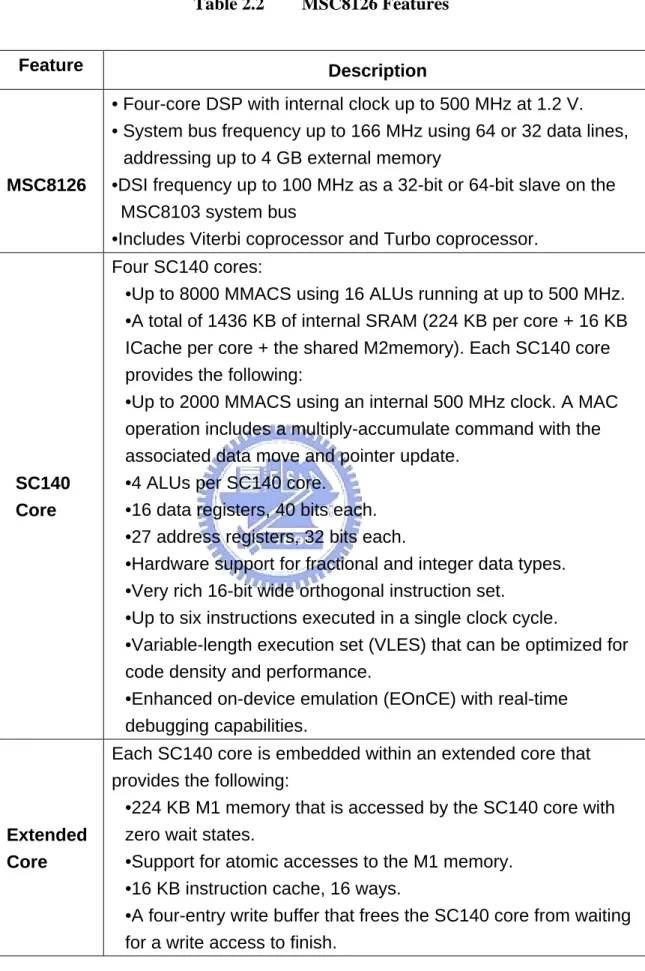
2.1.2 MSC8126 Features

The MSC8126 (see Fig. 2.2) is a highly integrated system-on-a-chip that combines four SC140 extended cores with a turbo coprocessor (TCOP), a viterbi coprocessor (VCOP), an RS-232 serial interface, four time-division multiplexed (TDM) serial interfaces, thirty-two general-purpose timers, a flexible system interface unit (SIU), an Ethernet interface, and a multi-channel DMA controller.

The SC140 extended core (see Fig. 2.3) is a flexible, programmable DSP core that handles compute-intensive communications applications, providing high performance, low power, and code density. It efficiently deploys a novel variable-length execution set (VLES), attaining maximum parallelism by allowing multiple address generation and data arithmetic logic units to execute multiple operations in a single clock cycle. A single SC140 core running at 500 MHz can perform 2000 MMACS. Having four such cores, the MSC8126 can perform up to 8000 MMACS per second.

Based on [7], we organized the features of MSC8126 and SC140 extended core and listed them in Table 2.2. The block diagram of the MSC8126 is shown in the Fig. 2.2 and SC140 extended core is shown in the Fig. 2.3.

Table 2.2 MSC8126 Features Feature _Description

MSC8126

• Four-core DSP with internal clock up to 500 MHz at 1.2 V. • System bus frequency up to 166 MHz using 64 or 32 data lines,

addressing up to 4 GB external memory

•DSI frequency up to 100 MHz as a 32-bit or 64-bit slave on the MSC8103 system bus

•Includes Viterbi coprocessor and Turbo coprocessor.

SC140 Core

Four SC140 cores:

•Up to 8000 MMACS using 16 ALUs running at up to 500 MHz. •A total of 1436 KB of internal SRAM (224 KB per core + 16 KB ICache per core + the shared M2memory). Each SC140 core provides the following:

•Up to 2000 MMACS using an internal 500 MHz clock. A MAC operation includes a multiply-accumulate command with the associated data move and pointer update.

•4 ALUs per SC140 core. •16 data registers, 40 bits each. •27 address registers, 32 bits each.

•Hardware support for fractional and integer data types. •Very rich 16-bit wide orthogonal instruction set.

•Up to six instructions executed in a single clock cycle.

•Variable-length execution set (VLES) that can be optimized for code density and performance.

•Enhanced on-device emulation (EOnCE) with real-time debugging capabilities.

Extended Core

Each SC140 core is embedded within an extended core that provides the following:

•224 KB M1 memory that is accessed by the SC140 core with zero wait states.

•Support for atomic accesses to the M1 memory. •16 KB instruction cache, 16 ways.

•A four-entry write buffer that frees the SC140 core from waiting for a write access to finish.

Multi-Core Shared Memories

•M2 memory (shared memory):

—A 476 KB memory working at the core frequency. —Accessible from the local bus.

—Accessible from all four SC140 cores using the MQBus. •4 KB bootstrap ROM.

2.2 Developing Optimized Code for Speed on the

SC140 Cores

Speed optimization techniques on the SC140 core are generally classified as follows [8]:

• Loop unrolling • Split computation • Multisampling

2.2.1 Loop unrolling

The most popular speed optimization technique, loop unrolling explicitly repeats the body of a loop with corresponding indices. As a stand-alone technique, loop unrolling increases the Data ALU usage per loop step. If the iterations are independent, each one is performed on a single Data ALU. For example, the following code unrolls the loop three times to create four operations to be executed per one loop step:

Example 1. Loop Unrolling

Word16 signal[SIG_LEN]; #pragma align signal 8

for ( i = 0; i < SIG_LEN; i+=4 )

{ signal[i+0] = L_shr(signal[i+0], 2); signal[i+1] = L_shr(signal[i+1], 2); signal[i+2] = L_shr(signal[i+2], 2); signal[i+3] = L_shr(signal[i+3], 2); }

In this document, the unroll-factor refers to the number of copies of the original loop that are in the unrolled loop. For example, in Example 1, the unroll-factor is 4.

2.2.2 Split Computation

A frequent operation in DSP computations is to reduce one dimension of a data massive (scalars are zero-dimensional, vectors are one-dimensional, and matrices are two-dimensional). The most frequently used reductions are: energy computation of a vector, mean square error, or maximum of a vector. If the reduction operator is associative and commutative, the reduction can be performed by splitting the original data massive into several data massives (usually four on the SC140 core). The reduction is applied to the smaller massives, and the results are combined to obtain the result as shown in Example 2.

Example 2. Split Computation

/* Energy computation for the signal[] vector of */ /* size SIG_LEN (multiple of 4). */

L_e0 = L_e1 = L_e2 = L_e3 = 0;

for ( i = 0; i < SIG_LEN; i+=4 ) {

L_e0 = L_mac(L_e0, signal[i+0], signal[i+0]); L_e1 = L_mac(L_e1, signal[i+1], signal[i+1]); L_e2 = L_mac(L_e2, signal[i+2], signal[i+2]); L_e3 = L_mac(L_e3, signal[i+3], signal[i+3]); }

L_e0 = L_add(L_e0, L_e1); L_e2 = L_add(L_e2, L_e3); L_e0 = L_add(L_e0, L_e2);

The same conditions must be met as for loop unrolling (for example, the vector alignment and the loop counter). In addition, split computations are used if the operator on the given data set is associative and commutative.

2.2.3 Multisampling

The multisampling technique is frequently used in nested loops and is a combination of primitive transformations. Given a nested loop formed out of OL (outer loop) and IL (inner loop containing one or two instructions), the multisampling transformation consists of the following:

•A loop unroll applied for OL to create a new OL with four IL inside (IL0, IL1, IL2, and IL3)

•A loop merge applied for IL0, IL1, IL2, and IL3 to create a new IL that makes more efficient use of the DALU units.

•A loop unroll applied to the newly-obtained IL so that the programmer can detail the reuse of already fetched values in the computations inside the new IL.

In Example 3, the nested loop computes the maximum absolute value of the correlations between X[] and h[]:

Example 3. Code Before Multisampling

L_max = 0;

for (i = L_SUBFR-1; i >= 0; i--) {

L_s = 0; for (j = i; j < L_SUBFR; j++){ L_s = L_mac(L_s, X[j], h[j-i]); } y32[i] = L_s; L_s = L_abs(L_s); if( L_s > L_max ) { L_max = L_s; } }

Example 4 shows the result of applying the multisampling technique. The speed

and size estimations are not as obvious as they are for loop unrolling and split computation. We have the following before multisampling:

Example 4. Code After Multisampling

L_max0 = L_max1 = L_max2 = L_max3 = 0;

for (i = L_SUBFR-4; i >= 0; i-=4){

Word16 x_curr = X[i];

L_s0 = L_s1 = L_s2 = L_s3 = 0; h0 = h[0]; h1 = h2 = h3 = 0; for (j = i; j < L_SUBFR; j+=4){ L_s0 = L_mac(L_s0, x_curr, h0); L_s1 = L_mac(L_s1, x_curr, h1); L_s2 = L_mac(L_s2, x_curr, h2); L_s3 = L_mac(L_s3, x_curr, h3); h3 = h[j+1-i]; x_curr = X[j+1]; L_s0 = L_mac(L_s0, x_curr, h3); L_s1 = L_mac(L_s1, x_curr, h0); L_s2 = L_mac(L_s2, x_curr, h1); L_s3 = L_mac(L_s3, x_curr, h2); h2 = h[j+2-i]; x_curr = X[j+2]; L_s0 = L_mac(L_s0, x_curr, h2); L_s1 = L_mac(L_s1, x_curr, h3); L_s2 = L_mac(L_s2, x_curr, h0); L_s3 = L_mac(L_s3, x_curr, h1); h1 = h[j+3-i]; x_curr = X[j+3]; L_s0 = L_mac(L_s0, x_curr, h1); L_s1 = L_mac(L_s1, x_curr, h2); L_s2 = L_mac(L_s2, x_curr, h3); L_s3 = L_mac(L_s3, x_curr, h0); h0 = h[j+4-i]; x_curr = X[j+4]; } L_y[i ] = L_s0; L_y[i+1] = L_s1; L_y[i+2] = L_s2; L_y[i+3] = L_s3; L_s0 = L_abs(L_s0); L_s1 = L_abs(L_s1); L_s2 = L_abs(L_s2); L_s3 = L_abs(L_s3); L_max0 = L_max(L_max0, L_s0); L_max1 = L_max(L_max1, L_s1); L_max2 = L_max(L_max2, L_s2);

L_max3 = L_max(L_max3, L_s3); }

L_max0 = L_max(L_max0, L_max1); L_max1 = L_max(L_max2, L_max3); L_max0 = L_max(L_max0, L_max1);

The speed increases by sample-factor times, but the code size also increases significantly. Therefore, multisampling should be used only if the speed constraints are much more important than the size constraints.

Chapter 3 Channel Estimation

Techniques for IEEE 802.16e

Downlink and DSP Implementation

In this chapter, we introduce three algorithms of channel estimation for IEEE 802.16e OFDMA transmission system and evaluate the performance of each channel estimation method mainly by the bit error rate (BER) and the mean square error (MSE).

This chapter is organized as follows. In section 3.1, we present the algorithms of channel estimation. In section 3.2, we introduce our simulation environment. In section 3.3, we show floating-point simulation figures of all algorithms. In section 3.4, we show performance tables and fixed-point simulation figures which implement in DSP. Section 3.5 is the WiMAX system integration on the DSP platform.

3.1 Channel Estimation Techniques for 802.16e

Downlink

In IEEE 802.16e OFDMA-PHY downlink PUSC, the sub-carriers are divided into many clusters containing 14 adjunct sub-carriers each. Fig 3.1 depicts this cluster structure and the position of pilot sub-carriers in each cluster for even or odd symbol. According to the pilot arrangement, we adopt three different techniques to estimate

channels and discuss in following sections.

Fig. 3.1 Cluster structure [9].

3.1.1 Channel estimation with linear interpolation (LI)

The received signal y_k (with cyclic prefix removed) can be expressed as

1 , 0

,0

1

L k k l k l k l

y

h x

w

k

N

− − =

=

∑

+

≤ ≤ −

_(3.1)

where

h

k l, represents the lth channel tap ( 0≤ ≤ − L represents the number of l L 1, all channel taps) and

x

k l− represents (k−l)th sample of the transmitted signal and

k

w

represents the additive white Gaussian noise and N is FFT size. Taking an FFT of

k

y , we obtain the received signal in frequency domain:

1 , , 0,

, 0

1

N i i i i i m m i m m i

Y

H X

H

X

W

i

N

− = ≠

=

+

∑

+

≤ ≤

−

(3.2) where 2 ( ) 2 1 1 , , 0 0

1

L N j k i m j lm N N i m k l l k

H

h e

e

N

π − π − − _{− −} = =

=

∑ ∑

_{. (3.3)} i

When m ≠ i, Hi m, represents the effect of X onm Yi. So we can see clearly here

how ICI is introduced by the time-varying channel. In the following, we just use linear interpolation techniques to estimateH . i i_,

Fig. 3.2 Pilot distribution in successive clusters [9].

We ignore H_{i m,} (m ≠ i) in (3.3), then estimate H . This can be done by i i_,

Step 1) Estimating H at pilot positioni i_,

i

n, which means to obtain all the

frequency responses at the black sub-carriers in each cluster shown in Fig. 3.2, could be written as

,

ˆ

n n n n l i l i i l i

Y

H

X

=

(3.4) where the superscript l represents the symbol index.

Step 2) Interpolating between symbols, we obtain all frequency responses at the brown sub-carriers in different clusters shown in Fig. 3.2.

The Hˆi il_n,_nwill be obtained by linear interpolation as follows:

(

1 1

)

, , ,

1

ˆ

ˆ

ˆ

2

n n n n n n l l l i i i i i i

H

=

H

−

+

H

+ _{. (3.5)}

equal-spaced distribution. In order to obtain all the frequency responses at the white sub-carriers in different clusters shown in Fig. 3.2, we do linear interpolation once again as follows

1 1 , , ,

4

ˆ

ˆ

ˆ

4

4

n n n n n n l l l i k i k i i i i

k

k

H

H

H

+ + + +

−

=

+

_{. (3.6)}

Note we use the same method to perform extrapolation for out of range values which are on the edge of clusters.

Step 4) This is the final step to estimate the transmitted frequency data as follows: ,

ˆ

ˆ

l l i i _l i i

Y

X

H

=

_{. (3.7)}

For the above steps, we know how to use linear interpolation with pilots. If we use preamble to estimate channel frequency response, our equation is similar to (3.6) because of preamble structure (see Fig. 1.11). Simulation results are shown and discussed in the back section.

3.1.2 Channel Estimation with circular interpolation

(CI)

Circular interpolation [14] is the ability to interpolate values around a circular trajectory. We treat all complex values as the form of

r

×

e

jθ, which r is the radius and θ is the phase in complex plane. In the section, we do linear interpolation in the radius and phase, but we get the complex values which aren’t interpolated linearly in real and imaginary part. Therefore, the algorithm which is discussed in section 3.1.1 can be employed here and repeat all steps in the phase and radius. Simulation results

are shown and discussed in the back section.

3.1.3 Least-Square (LS) Estimator with time-domain

linear interpolation

The algorithm of least-squares channel estimation mainly estimates time-varying channels. In a time-varying environment, it amounts to estimating N channels

h : [

_,0

, ,

_{, 1}

] ,0

T

1

k

=

h

k

…

h

k L−

≤ ≤ −

k

N

; in other words, we need to estimate

N×L parameters. We assume that there is not significant variation between channels 0

h

and

h

_N-1. In order to reduce complexity, we only estimate2 L× parameters which are

h

₀ and

h

_N-1 channels. Interpolating between channels

h

₀ and

h

_N-1, we obtain the remaining channels by linear interpolation. Based on [10], we use P pilot tones to estimate channels

h

₀ and

h

N-1 by least-squares method, but P must be

chosen such that P≥2L. Revisiting (3.3) for a pilot tone p, then the received

tone

Y

p would be

, , ,

noise

p p p p p q q n p n

q pilot n not pilot q p

Y

H

X

H

X

H

X

≠

=

+

∑

+

∑

+

_(3.8) which yields ,

b h

p

noise

p n p n n not pilot

Y

=

+

∑

H

X

+

,

b :

p

b

p q q q pilot

X

⎛

⎞

= ⎜

⎟

⎝

∑

⎠

(3.9) and the 2L × 1 vector

0 1

h :

h , h

T T T

N−

⎡

⎤

= ⎣

⎦

. (3.10) According to [10], we defined the

1 2

×

L

row vector

b

p q,

: (b , b )

=

₁p q, ₂p q, and the 1×L row vector

( )

(

)

, , ,

b

p q

:

p q

0 , ,

p q

1

m

=

⎡

⎣

b

m

…

b

m

L

−

⎤

⎦

(3.11) where

( )

1 , (2 / ) (2 ( ) / ) , 0

1

:

N p q j l N j r q p N m m r r

b

l

e

a

e

N

π − π − − =

=

∑

_{. (3.12)}

The number am r, is the linear interpolation coefficients between channels

h

0

and

h

N-1. For the above description, the pilot-based channel estimation can be

achieved by

Step 1) Revisiting (3.9), we can express the received tone

Y

p as

,

b h

: (

b )h noise

p p p p q p q q not pilot

Y

e

e

X

=

+

=

∑

+

(3.13) Step 2) Form the P × 2L system of linear equations

(1), (1) (1) (1) ( ), ( ) ( ) (1)

b

h+

b

p p p p p P p P p P p

Y

e

Y

e

⎡

⎤

⎡

⎤

⎡

⎤

⎢

⎥

⎢

⎥

⎢

⎥

= ⎢

⎥

⎢

⎥

⎢

⎥

⎢

⎥

⎢

⎥

⎢

⎥

⎣

⎦

⎣

⎦

⎣

⎦

(3.14) or Y = Bh + e.

Step 3) Obtain

h

as the least squares solution of the aforementioned system of linear equations (3.14).

For the above steps, we know how to estimate channels with least-squares method. Simulation results are shown and discussed in the back section.

3.1.4 ICI Cancellation by Equalization of Time-Varying

Channels

For mobile applications, channel variations within an OFDM block period destroy the orthogonality between sub-carriers; the effect, known as Inter-carrier Interference (ICI), will degrade the system performance. In [11], we use a block MMSE equalizer to cancel out the ICI. The received signal Y could be expressed by

Y= ΛX + noise (3.15) where Y is the N × 1 received vector, X is the N × 1 transmitted vector, and Λ is the N × N frequency-domain channel matrix as below

0,0 1,0 1,0 0,1 1,1 1,1 0, 1 1, 1 1, 1 N N N N N N

H

H

H

H

H

H

H

H

H

− − − − − −

⎡

⎤

⎢

⎥

⎢

⎥

Λ=

⎢

⎥

⎢

⎥

⎣

⎦

. (3.16)

All elements of Λ channel matrix could be estimated by LS channel estimation, which had introduced in section 3.1.2. Linear block MMSE equalization could be expressed by

(

₁

)

1 MMSE

ˆX

H H

I

Y

N

γ

− −

= Λ ΛΛ +

_(3.17)

where γ is the signal-to-noise ration (SNR), IN is the N-dimension identity matrix,

and the superscript H represents the conjugate and transposed matrix. The transmitted signal X could be recovered by (3.17). In fact, we are unable to estimate time-varying channel matrix accurately so that the effect of ICI cancellation is not good. Simulation results are shown and discussed in the following sections.

3.1.5 Computational Complexity Analysis

Table 3.1 is the computational complexity analysis of all algorithms. Note that

Nused is the number of all data sub-carriers and N is the FFT size and Np is the number

of all pilots and L is the number of all channel taps. The computational complexity of phase and amplitude is calculated by CORDIC algorithms [13] and quantified by 14-bit. And the matrix inversion in (3.17) requires

( )

3

O N flops.

Table 3.1 Computational Complexity

Algorithm Complexity Comments

Linear interpolation 2×Nused

multiplications

Low complexity Circular interpolation

2

×

N

used

+ × ×

2 14

N

P

multiplications

Moderate complexity Least-Square estimator with

time-domain linear interpolation

( )

3 ₂ 2L +8L ×N_P+2L N× _P complex multiplications High complexity ICI cancellation 3 2 3 N× +N complex multiplications Very high complexity

3.2 Simulation Channel Model and OFDMA

Downlink System Parameters

In the section, we gives the parameters and introduce the channel model [12] used in our simulation work as follows.

z Primitive Parameters

The following four primitive parameters defined in [4] characterize the OFDMA symbol:

1) BW: This is the nominal channel bandwidth.

2) Nused: Number of used sub-carriers (which includes the DC sub-carrier).

3) n: Sampling factor. This parameter, in conjunction with BW and Nused

determines the sub-carrier spacing, and the useful symbol time. This value is set as follows: for channel bandwidths that are a multiple of 1.75 MHz then n = 8/7 else for channel bandwidths that are a multiple of any of 1.25, 1.5, 2 or 2.75 MHz then n = 28/25 else for channel bandwidths not otherwise specified then n = 8/7.

4) G: This is the ratio of CP time to “useful” time. The following values shall be supported: 1/32, 1/16, 1/8, and 1/4.

z Derived Parameters

The following parameters are defined in terms of the primitive parameters: 1) NFFT: Smallest power of two greater than Nused

2) Sampling frequency:Fs =⎢⎣n BW⋅ / 8000⎥⎦×8000 3) Sub-carrier spacing:Δ =f F_s/N_FFT

4) Useful symbol time:Tb = Δ 1/ f 5) CP time:T_g = ⋅ G T_b

6) OFDMA symbol time:T_s = + T_b T_g

7) Sampling time:T_b/N_FFT

Table 3.2 OFDMA Downlink Parameters

Parameters Values System Channel Bandwidth 5 MHz

FFT Size (NFFT) 512

Used sub-carriers (Nused) 420

G (ratio of CP) 1/8 Sampling factor n 28/25 Number of Sub-channels 8 Central frequency 2.5 GHz Tone spacing 10.9375 kHz Guard Time 11.43 μs Useful symbol time 91.4286 μs OFDMA Symbol Duration 102.86 μs

Table 3.3 Terrain Type vs. SUI Channels

Terrain Type SUI Channels C: flat terrain, light tree SUI-1, SUI-2 B: between A and C SUI-3, SUI-4 A: hilly terrain, heavy tree SUI-5, SUI-6

Table 3.4 General Characteristic of SUI Channels

Doppler Low Delay Spread Moderate Delay Spread High Delay Spread Low SUI-1, SUI-2, SUI-3 SUI-5

High SUI-4 SUI-6

Erceg et al [12] proposed a total of six different radio channel models for fixed wireless applications in three terrain categories. We show three terrain categories corresponded with the SUI channels in Table 3.3 and general characteristic of SUI

channels in Table 3.4. For the above SUI channels, we employ SUI-3 model in our simulation, but we use Rayleigh fading to model all the paths in these channels. The channel characteristics are shown in Table 3.5.

Table 3.5 SUI-3 Channel Model

Tap 1 Tap 2 Tap 3 Units Delay 0 0.4 1.1 μs

Power 0 -12 -15 dB

Doppler 0.2 0.15 0.25 Hz

3.3 Performance of Channel Estimation

3.3.1 Simulation Flows

Fig. 3.3 illustrates our simulated system. We assume perfect synchronization in our simulation. After channel estimation, we calculate the mean square error (MSE) between the real and estimated channel, where the average is taken over the sub-carriers. The bit error rate (BER) can also be obtained after de-mapping.

FEC Framing IFFT Power Control Channel Simulator (SUI-3)

SYNC. FFT Channel

Estimation De-framing De-FEC

3.3.2 Floating-point Simulation

All of our simulated figures are in SUI-3 channel with different velocity of QPSK. Fig. 3.4 and Fig. 3.5(a) show MSE curves of different algorithms which are linear interpolation, circular interpolation, least-squares method. Fig. 3.4 is estimated by preamble and the following figures of performance are estimated by pilots. We can find that the performance showed in Fig. 3.4 is better than Fig. 3.5(a) due to different number of training data. Fig. 3.5 shows MSE and BER curves of different algorithms with different Doppler frequency. We can see that LS channel estimation had best performance among three different algorithms. The reason can be explained by Fig. 3.6, which shows the estimated channel frequency responses of all algorithms. Based on our observation of Fig. 3.6, the curve of frequency responses which estimated by the LS algorithm is smooth at sharp curves and better performance than other algorithms. Furthermore, CI algorithm seems to be good performance, but it has worse performance when the channel’s gain is near zero. Besides, LS algorithm can cancel partial ICI at the pilot positions, but its effect is not obviously owing to the distance between pilots. Fig. 3.7 shows that the influence of carrier frequency offset (CFO) on different algorithms in BER is slight. Fig. 3.8 and Fig. 3.9 display the performance of a cluster in even and odd symbols. As for LI and circular interpolation, the pilot positions of both even and odd symbols have higher MSE but BER is zero in time-invariant channel. The reason of higher MSE at pilot positions may be that the noise be cancelled by interpolation. The channel responses estimated by LS is so smooth that its curves of Fig. 3.9 have no big change in time-invariant channel. Fig. 3.10 illustrates the effect of ICI cancellation algorithm is not obvious because of inaccurate channel estimation. If we consider the influence of CFO in ICI cancellation

algorithm, we can find that the effect of ICI almost has no improvement in performance from Fig.3.11. Since we know the importance of accurate channel estimation, we should search other more accurate methods of channel estimation for our future work.

Fig. 3.4 The comparison of different SUI-3 channel estimated methods in performance (Using Preamble).

(a)

(b)

Fig. 3.5 The comparison of different SUI-3 channel estimated methods in performance. (a) MSE. (b) BER.

Fig. 3.6 The comparison of channel frequency responses which are estimated by different algorithms.

Fig. 3.7 BER performance of different algorithms with various velocities and CFO = 0.02 × tone spacing frequency.

(a)

(b)

Fig. 3.8 Average cluster BER performance in SUI-3 at 30 dB SNR. (a) Odd symbol. (b) Even symbol.

(a)

(b)

Fig. 3.9 Average cluster MSE performance in SUI-3 at 30 dB SNR. (a) Odd symbol. (b) Even symbol.

Fig. 3.10 Performance of ICI cancellation algorithm with various velocities.

Fig. 3.11 Performance of ICI cancellation algorithm with various velocities & CFO = 0.02 × tone spacing frequency.

3.4 DSP Implementation

3.4.1 Implementation of Transmitter

The PHY subsystem on the MSC8126 includes the user domain processing (UP), the frequency domain (FP) processing, and the time domain processing (TP). The user domain processing covers the channel encoding and decoding steps (see 8.4.9 of [3]-[4]). Specifically channel encoding steps are randomization, convolutional encoder, interleaving, constellation mapping. Fig. 3.12 shows an overview of UP and FP steps throughout the PHY chain on the MSC8126.

Randomizer FEC Encoder Interleaver QAM Modulation Pilot Generation Pilot Insertion MAC layer

TX User SP TX Frequency _{Domain SP}

User Multiplexing

to TP

Fig. 3.12 DL UP and FP chain on MSC8126.

The frequency domain processing is mainly responsible for the OFDMA signal formatting. It is a subsystem that is not tied to any specific user functionality. The processing steps in the DL direction are:

z Preamble generation z Data modulation

z Data symbol mapping

z Pilot generation and mapping z Carrier scrambling

From a processing point of view, the DL FP data flow is as follows and shown in Fig. 3.13.

(1) The first symbol in a frame is the preamble, which is a PN code pattern dependent on some control variable like ID cell. It is independent of user data. The mobile station knows this sequence and hence may use for initial channel estimation.

(2) After the preamble user processing fills sub-channels with user and control data. FP performs as follows and is shown in Fig. 3.14 for detail.

z Mapping data to logical slots on logical sub-channels (function MapDl). z Generate and insert the pilot symbols into the tiles.

z Translate the logical carriers to physical carriers by the function CarrierScrambler(). This function needs a permutation table, which is called ausiDlCarrierMap. This map is generated once per permutation zone.

z Modulate the resulting data vector on the physical carriers by a PN sequence and a static weight. This is achieved by the function DataModulation.

MapDl()

Map user bursts on frames in the symbol sub-channel space

(see [1..3]. sec 8.4.3.4)

CarrierScrambler()

Scramble carrier by using look-up table

To IFFT From DL User processing

Carrier Lookup table:

ausiDlCarrierMap[] GenerateDlTable(..)

Generate Carrier Lookup Table (see [1..3]. sec 8.4.6.1.2.2.2) Map Information PreambleGen() Preamble Generation (see [1..3]. sec 8.4.6.1.1) From DL User processing Map Information To IFFT DataModulation() RCF-IF MapToComplexRowVec tor()

Fig. 3.13 DL processing functions.

14 adjacent Carriers 14 adjacent Carriers 14 adjacent Carriers 14 adjacent Carriers N-Used/14 physical Cluster 14 adjacent Carriers 14 adjacent Carriers 14 adjacent Carriers 14 adjacent Carriers N-Used/14 locical Cluster First Perm Formula: Cluster Scrambling Major Group 0 Major Group 5 locical Cluster 0-> N-1 locical Cluster 5N-> 6N-1 N=24 for FFT2048 N=12 for FFT1024 N=10 for FFT512 N=2 for FFT128 N-Used physical Carriers Linear ordered data carriers All Carriers except pilots All Carriers except pilots Second Perm Formula: Carrier Scrambling Linear ordered data samples DL User Processing Physical to logical

The time domain processing includes IFFT/FFT and synchronization mechanism. Our DSP implementation is limited to only PUSC and not considered that the configurations marked as "optional" in [3] and [4]. This functionality is confined to user independent sub-channel management. Hence, all specific control channels like ranging, FCH, Map-DL/UL bursts etc are not considered specifically because they are treated as normal bursts.

Table 3.6 and Table 3.7 list the cycle count of UP and FP respectively for WiMAX OFDMA DL transmitter on MSC8126. Fig. 3.15 and Fig. 3.16 show the histograms of Table 3.6 and Table 3.7 respectively. Some functions in Table 3.6 has assemble code to reduce execution time such as Randomizer, Convolutional Encoder, Puncture and Interleaver. Note that data symbol rate is not included preamble symbol and data initialization in Table 3.7, because they must be done only once at first.

Table 3.6 Cycle Count of DL UP

Function Cycle Count (cycles/bit) Randomizer (assembly) 0.15

Randomizer 0.23

Convolutional Encoder (assembly) 1.02 Convolutional Encoder 2.21 Puncture (Rate = 1) (assembly) 0.45 Puncture (Rate = 1) 0.71 Interleaver (assembly) 13.64

QPSK Modulation 15.95 Total Cycles (assembly) 18.59 Bit Rate (Mbits/sec) 26.39

Cycle count of UP functions

0 2 4 6 8 10 12 14 16 18 20 C lo ck cy cl es p er b it Randomizer (assembly)

Convolutional Encoder (assembly) Puncture (Rate = 1) (assembly) Interleaver (assembly)

QPSK Modulation Total Cycles

Total

Fig. 3.15 Histogram of UP function cycle count.

Table 3.7 Cycle Count of DL FP

Function Description Function Name Cycle Count Preamble

Symbol Preamble Generation PreambleGen() 4175 Carrier Permutation Table

Generation GenerateDlTable() 98089 Initial Data Position within

Sub-channel InitialDataPositionVectorDl() 1360 Data

Initialization

Subtotal Cycles 99508

Mapping Data onto Physical

Sub-carrier MapDl() 3147 Carrier Scramble CarrierScramble() 5661 Carrier Manipulation DataModulation() 10945 Data Symbol

Subtotal Cycles 23990

Total Cycles 135549

Data Symbol Rate (symbols/sec) 20842

Cycle count of FP functions 0 20000 40000 60000 80000 100000 120000 140000 160000 C lo ck cy cl es PreambleGen() GenerateDlTable() InitialDataPositionVectorDl() MapDl() CarrierScramble() DataModulation() Total

Fig. 3.16 Histogram of FP function cycle count.

3.4.2 Implementation of Receiver at channel estimation

FEC Framing IFFT Power Control Channel Simulator (SUI-3)

SYNC. FFT Channel

Estimation De-framing De-FEC Simulation system input

Simulation system output

Fig. 3.17 Simulation system.

Fig. 3.18 described that we pointed out the simulated input and output positions in our simulation system. Here we assumed that synchronization was perfect. As a result of consideration to complexity, we implemented channel estimation techniques

described in section 3.1.1 for WiMAX OFDMA downlink on MSC8126 DSP. Note that all simulated parameters were the same as section 3.3.2.

Fig. 3.19 illustrates the performance of 16-bit fixed-point computation compared with floating-point computation in SUI-3 at different Doppler frequencies. We could see that there was almost no difference between floating-point and 16-bit fixed-point computation. The implementation results of channel estimation are shown in Table 3.8 and Fig. 3.20, and we see that execution time of channel estimation can be completed with one symbol duration. Note that symbol duration T =102.9μsec in Table 3.7. S

Fig. 3.18 Performance of comparison between floating-point and fixed-point computation in SUI-3 for various Doppler frequencies with preamble.

(a)

(b)

Fig. 3.19 Performance of comparison between floating-point and fixed-point computation in SUI-3 for various Doppler frequencies. (a) BER. (b) MSE.

Table 3.8 Cycle Count of Channel Estimation

Process Cycle Count (cycles/symbol) Time (μsec/symbol) One-tap Equalization at pilot

positions 1283 2.57 (0.025×T ) S Linear Interpolation between pilot

positions 2624 5.25 (0.051×T ) S Total 3907 7.82 (0.076×T ) S

Cycle Count of Channel Estimation

0 5000 10000 15000 20000 25000 Clock Cycles One-tap Equalization at pilot positions Linear Interpolation between pilot positions Total

Fig. 3.20 Histogram of Channel Estimation function cycle count.

3.5 WiMAX System Integration on the DSP Platform

From above sections, we have showed the cycle count of each function respectively in WiMax system except for synchronization. In this section, we attempt to combine all functions including synchronization, and test whether the total cycle count achieve real time requirements. Table 3.9 and Table 3.10 show the throughput of transmitter and receiver respectively. The theoretical maximum throughput of WiMAX technology could support approximately 75 Mbps per channel (in a 20 MHz channel

using 64-QAM 3/4 code rate), but our simulated parameters only could achieve approximately 4.7 Mbps per channel (in a 5MHz channel using QPSK 1/2 code rate). In Table 3.9, the transmitter throughput is about 7.79 Mbps and achieved real time requirements. In Table 3.10, the synchronization cost the most cycles and waited for 12 symbol durations. Maybe we could use optimized assembly codes or multi-core DSP to reduce waiting time.

Table 3.9 Throughput of WiMAX 16e Transmitter on MSC8126

Process Cycle Count (cycles/bit) Time (μsec/bit) Throughput (Mbps) UP (Rate = 1/2) 18.59 0.037 26.89

FP 23990/840 = 28.56 0.057 17.51 IFFT-512 3970/840 = 4.73 0.009 111.11

Add CP 10968 cycles/symbol n/a n/a Tx 53944/840 = 64.22 0.128 7.79

Table 3.10 Cycle Count of WiMAX 16e Receiver on MSC8126

Ts = 102.9μsec

Process Cycle Count (cycles/symbol) Time (μsec/symbol) Synchronization 65406 130.81 (1.27×T ) _S

FFT-512 3970 7.94 (0.077×T ) _S Channel Estimation 3907 7.82 (0.076×T ) _S Rx 73283 146.57 (1.424×T ) _S

Chapter 4

Conclusions and Future Work

4.1 Conclusions

In this thesis, I have presented three channel estimation methods and one ICI cancellation algorithm for IEEE 802.16e downlink. The proposed methods utilized the pilots or the preamble structure to obtain channel frequency responses. The first method is to do linear interpolations in the time and frequency domain. The second method is to do circular interpolations which are similar to LI in radius and phase. The final method is to obtain the channel estimations at the beginning and the end of an OFDM symbol then interpolate between them linearly. The final method is also accompanied by an MMSE equalization to reduce the effect of ICI. Simulation results show that under the 802.16e downlink environment, the LS method provides very limited performance advantages while suffers from tremendous increase of computational complexity. The linear interpolation algorithm is, therefore, chosen as the channel estimation method in the DSP implementation.

Our main work is the DSP implementation of an 802.16e WiMAX OFDMA downlink system including the transmitter and receiver. After system integration and DSP implementation, the transmitter throughput is close to 7.79 Mbps and achieves minimum real time requirements. However, the receiver processing of initialization