Optimal software release policy based on cost and reliability with testing efficiency

(1)

Optimal Software Release Policy Based on Cost and Reliability with

Testing Efficiency

Chin-Yu Huang', Sy-Yen Kuo', and Michael R. Lyu2

'Department of Electrical Engineering

National Taiwan University

*Computer Science

&

Engineering Department

The Chinese University of Hong Kong

Taipei, Taiwan

Shatin, Hong Kong

sykuo@cc.ee.ntu.edu.tw

lyu@cse.cuhk.edu.hk

Abstract

In this paper, we study the optimal software release problem considering cost, reliability and testing eficiency. We first propose a generalized logistic testing-effort function that can be used to describe the actual

consumption of resources during the sojiware development process. We then address the problem of how to decide when to stop testing and when to release software f o r use. In

addressing the optimal release time, we consider cost and reliability factors. Moreover, we introduce the concept of testing eficiency, and describe how reliability growth models can be adjusted to incorporate this new parameter. Theoretical results are shown and numerical illustrations are presented.

I. Introduction

For a large-scale or international software company, successful development of a software system depends on its software components. Therefore, the reliability of a large software system needs to be modeledtanalyzed during the software development process. The future failure behavior of a software system is predicted by studying and modeling its past failure behavior[l-31. It is very important to ensure the quality of the underlying software systems in the sense that they perform their functions correctly. Recently, we [4-51 proposed a new software reliability growth model which incorporates the concept of logistic testing-effort function into an

NHPP

model to get a better description on the software fault phenomenon. In this paper, we will extend the logistic testing-effort function into a more generalized form and show that the generalized logistic testing-effort function has the advantage of relating the work profile more directly to the natural structure of software development through experiments on real data sets. In practice, if we want to detect more additional faults, it is advisable to introduce new toolsltechniques, which are fundamentally different

from

the methods currently in use. The advantage of these methods is that they candesign/

propose several testing programs or automated testing tools to meet the client's technical requirements, schedule, and budget. If software companies can afford a bigger budget for testing and debugging, a project manager can maximize the software reliability. Hence the cost trade-off of new techniquesttools can be considered in the software cost model and viewed as the investment required to improve the long-term competitiveness. Therefore, in this paper, in addition to modeling the software fault-detection process, we will discuss the optimal release problem based on cost and reliability considering testing-effort and efficiency.

2. Testing-effort function and software

reliability modeling

2.1. Review of SRGM with logistic testing-effort

function

If we let the expected number of faults be N(t), with mean value function as m(t), then an SRGM based on NHPP can be formulated as a Poisson process:

[m(t)l" exp[-m(t)~

n!

Furthermore, if the number of faults detected by the current testing-effort expenditures is proportional to the number of remaining faults, then we have the following differential equation:

P , [ N ( r ) = n ] = , n=O, 1, 2,

....,

(1) M r ) 1

- x - = r x [ a - m ( t ) ]

where m(t) is the expected mean number of faults detected in time (0, t ] , w ( t ) is the current testing-effort consumption at time t , a is the expected number of initial faults, and 00 is the error detection rate per unit testing-effort at time t. Solving the above differential equation, we have

dt w ( t )

m(t)=a( l-exp[-r( W(t)- W(O))])=a( ~-exp[-rW(t)]) Recently, we [4-51 proposed a Logistic testing-effort

(2)

function to describe the possible test effort patterns. The current testing-effort consumption is

N h (3) - N h x e x p b ] (l+Aexpw]) (expt]+Aexpk;]) a 2 2 - 4 r o =

where

N

is the total amount of testing effort to be eventually consumed, 01 is the consumption rate of testing-effort

expenditures, and A is a constant.

The cumulative testing effort consumption of Logistic

testing-effort function in time (0, t] is N

1

+

A exp[-m]

W ( r ) = and W ( r )

=

cw(t)dt (4)

2.2. A generalized logistic testing-effort function

From the previous studies in [4-51, we know that the

Logistic testing-effort function (i.e. the

Parr

model [8]) is based on a description of the actual software development process and can be used to describe the work profile of software development. In addition, this function can also be used to consider and evaluate the effects of possible improvements on software development methodology, such as top-down design, stepwise refinement or structured programming. Therefore, if we relax some assumptions when deriving the original

Parr

model and take into account the structured development effort, we get a generalized

Logistic testing-effort function

N x d m

( 5 ) where K is the structuring index and its value is large for modeling well-structured software development efforts and

p

is a constant.

When ~ = l , the above equation becomes

w k ( r ) =

q-

N

2

l+Aexp[-m]

p

If

p

is viewed

as

a normalized constant and we have &2, the above equation is equal to Eq. (4) [SI. Similarly, if @lc+l, we get a more generalized and plain solution for describing the cumulative testing effort consumption in (7)

W ,( t ) = X- (6)

N time (0, t]:

W,

( r ) =

‘cJT+Aexp[-ahtl

3. New tooldtechniques for increased

efficiency of software testing

It is well known that when the software coding is completed, the testing phase comes next and it is a necessary but expensive process. Once all the detectable faults are removed from a new software, the testing team

will need to determine when to stop testing and make a software risk evaluation. If the results meet their requirement specifications and the related criteria are also satisfied, the team will adorn and announce that this software product is ready for releasing/selling. Therefore, adequately adjusting some specific parameters of a SRGM and adopting the corresponding actions in the proper time interval can greatly help us to speedup obtaining the desired solution. In fact, several existing approaches can satisfy our requirements. For example, we have discussed the applications of testing-effort control and management problem in our previous studies [4]. The methods we proposed can easily control the modified consumption rate of testing-effort expenditures and could detect more faults in the prescribed time interval. It means that the developers/ testers will devote all their available knowledge/energy to complete such tasks without additional resources. Alternative to controlling the testing-effort expenditures, we believe that new testing schemes will help achieving a given operational quality at a specific time. That is, through some new techniquedtools, we can detecthemove more additional faults (i.e. these faults may or may not cause any failure or they are not easily exposed during the test phase), although these new methods will increase the extra software development cost. In practice, if we want to detect more potential faults, we may introduce new techniques/tools that are not yet used, or bring in experts to make a radical software risk analysis. In addition, there are newly proposed automated testing tools/techniques for increasing test coverage and can be used to replace traditional manual software testing regularly. The benefits to software developers/testers include increased software quality, reduced testing costs, improved release time to market, repeatable test steps, and improved testing productivity. These techniques can make software testing and correction easier, detect more bugs, save more time, and reduce expenses significantly [3]. Altogether, we hope that the experts, automated testing tools or techniques could greatly help us in detecting additional faults that are difficult to find during regular testing and usage,

in

identifying and correcting faults more cost effectively, and in assisting clients to improve their software development processes. To conclude, we introduce a gain parameter (GP) to describe the behavior or characteristics of automated testing techniques/tools and incorporate it into the mean value function [ 111. Therefore, the modified mean value function is depicted in the following:

*

me(t) = a(l -exp[-roWk (t)]),t Z Ts

me(t) = ~ ( 1 - exp[-rWK (t)]), t

< Ts

< T (8) where Q is the gain parameter (GP) and T, is the starting time of adopting new techniques/tools.

Eq. (8) means that if CT increases, me(?) increases. Thus the gain of employing new automated techniques/tools is

(3)

t 2Ts

m ( t ) P = 0, t <Ts (9)

where P is the additional fraction of faults detected by using new automated tools or techniques during testing. Substituting Eq. (8) into Eq. (9) and rearranging the above equations, we obtain the estimated value of gain parameter: I (I+P)xexpFrW 4 t ) l - P (10) In fact, we can interpret the gain parameter from different views. If we make a premise that the main goal of automated techniques/tools is to testldebug software with less testing effort, then the gain parameter

cs

and the testing-effort are inversely proportional to each other. That is, they have a joint effect on the software development process. On the other hand, under same testing effort, introducing new automated tools/methods should help us in detectindremoving more additional faults which are hard to detect without these new methods. Actually the most important thing is how to provide enough information about these approaches to the test team. Before adopting these automated techniques/tools, we should get the quantitative information from the industrial data relative to the methods' past performance applied in other instances (i.e. the previous experience in software testing), or qualitative information from the subjective valuation of methods' attributes. Certainly, the methods' past performance in aiding the reliability growth should be considered in determining whether they will be successful again or not [ 111. The distribution of (T can be estimated by performing

various simulations based on actual data sets. Additionally, the test teams' capacity of exercising these techniques/tools and the related environmental profiles also play an important role in achieving the desired goals. Here, we illustrate the new parameter with one real numerical example. This data set is from Ohba [IO]. If we are given the data sets whose parameters for test-effort function are in Table 1, then we can analyze the distribution of the gain parameter in various ways as follows.

Table 1

:

Parameters of generalized logistic testing- effort function and mean value function

--

m, ( t ) - ( l + P )

{

p ' 0 9

*

1 I

-1 U = r x (Wdt)

-

WK(0))

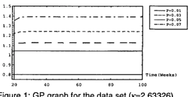
(about the 19th week), the number of faults detected is about 328. If we want to increase additional 0.01,0.03,0.05,0.07, 0.09, 0.1, 0.11 and 0.12 fraction of detected faults respectively, we must ensure that the gain parameter

cs

will be corresponding to growth as plotted in Fig. 1. That is, the performance and the related assistance of new tools/ methods should fit the growth curve as time progresses. If the trend fits, it means that through these new methods, we can adjust the consumption of testing-effort expenditures or raise the fault detection rate. In fact, in this data set, we find that at the end of testing, P=O.Ol, 0.02,.

..,

0.09,O.l or even 0.1 1, but P=O.12 is hard. The reason is that the value of 1- rn(t)/u controls the maximum possible value of P. That is, we should consider whether or not introducing new techniques/tools to detect additional faults only when the precondition: (1-m(t)/u)>P is satisfied. Finally, these tools or techniques we discussed have a big impact on software testing and reliability. In fact, they can provide the developers

or

test teams with feedback of useful information on the testing process for improvement as well as scheduling. However, we know that with more efficient testing, more time can be spent to make this software more reliable. Besides, introducing these new methods also requires that the original design of software be modified to get the best performance. Thereafter, the continued use of these tools/techniques can improve the software design.

G P -p=0.01 ---P=0.03 Pro. 07 c _ - - - _ -

---

-

- -

-

- -

- --

I

0 . 8 1 1T i m e (Weeks) 2 0 4 0 K O 8 0 1 0 0

Figure 1: GP graph for the data set

(e2.63326).

4. Optimal software release time

When the software testing is completed, software product is ready for release to users. However, proper timing is very important. If the reliability of the software does not meet the manager's goal, the developers or testers may request external help in testing. An optimal release policy for the proposed model based on such considerations is studied here.

4.1. Software release

time

based on cost criterion

47.850715709.2910.1399331 4 1414.4261 0.0398619

47.6561 114839.310.1365071 4.5 1416.1141 0.0397324 From

[IO],

we know that when the testing is completed

Okumoto and Goel [6] were the first to discuss the software optimal release policy from the cost-benefit viewpoint. Using the total software cost evaluated by cost criterion, the cost of testing-effort expenditures during

(4)

software development phase and the cost of correcting errors before and after release are:

CI(T) = C , m ( T ) + C 2 [ m ( T L C ) - m ( T ) ] + C 3 x ~ w ( x ) & Generally, in order to detect additional faults during testing, the test teamddebuggers may use new automated tools or techniques if they are available. Hence the cost trade-off of tools should be considered in software cost model. But they thereby save some of the greater expense of correcting errors during operation. By summing up the above cost factors, the modified software cost model is

a n

= C,(T)

+

c,

x ( l +

P )

x

m(T)

+

c,

[m(T,)

-

(1

+

P)

x m(T)J +

c,

x

l:

W(X)& (11) where Co(T) is the cost function of including automated tools/techniques to detect an additional fraction P of faults during testing.

In fact, the cost of a new tool or technique Co(T) may not be a constant during the testing phase of software development process. Moreover, in order to determine the testing cost C,(T), the most general cost estimating technique is to use the parametric methods if there are some meaningful data available. By differentiating Eq. (1 1) with respect to T and let

C,

(1 +P)=

C,'

and C, (1 +P)= C2*, we have

d d

*

-C2(T) = -Co(T)+C, am(T)exp[-rW*(T)]

d T dT

*

-C, am(T)xexp[-rW (T)]+C, xw(T) (12) However, the assumption that Co(r) is a constant may not be realistic in many situations. In addition, the assumption may lead to ill-defined testing. Therefore, we relax this assumption and explore the results. Here we propose two possibilities for Co(T) in order to interpret the cost consumption: (1) Co(T) is a constant [5], and (2) CJT) is proportional to the expenditures of testing-effort. The second assumption considers that Co(T) is a convex non- decreasing function of testing time t and initially is zero, while the time in progress increases linearly or non-linearly. For example, if in addition to introducing new automated tools/ techniques, we also adopt effective approaches from senior mentors in a professional software consultant company. Normally the testers can solve general problems by themselves when faults occur. But if some problems are so difficult to solve, they must ask the consultants to get more proper solutions. Therefore, we can conceive that such extra cost may include travel expenses to clients, charges for the phone support or root cause analysis of software faults, etc [3]. Sometimes they also provide the services for code inspections, diagramming, unit testing, and test planning. Generally, if using good automated approaches for software fault detection or usefuVpowerfu1 supports during software development becomes available, the testers can detect more faults. But the cost will be higher. Therefore, if C,(T) =

CO,

+CO

x(fAw(t)dt)",

T 2 TS and Co(T)= 0, T<T,, then we get

d

*

-C2(T) = w(t)x[ar(C, -C , )xexp[-rW (t)J+

dT

C,

+

CO

x m x

(I;

w(t)dr)" -

'1.

Since w(r)>O for 0 I T <

-

,

therefore, -C2(T)=O if P(T) 1

(ar(C2 - C , ) e ~ p [ - r W * ( t ) ] - C ~ r n ( ~ ~ w ( t ) d r ) ~ - ' ) = C3 (13) The left-side in Eq. (13) is monotonically decreasing function of T. Therefore, if

urx(C,

-

C, )expkr(W(Ts) - W(O))]>

C,

and P(TLc)<C,, it means that there exists a finite and unique solution To satisfying Eq. (13) which can be solved by numerical methods. It is noted that

-

C2(T) <O for 0 I

d dT

*

d dT

I

T <

T,

d

and -C2(T) >O for

DT,.

Thus, T=To minimizes C2(T)

dT

for To <TLC

4.1.1. Numerical Example 1. Here we illustrate how to minimize the software cost in which the new automated tooldtechniques are introduced during testing. From the previous estimated parameters for the data set in Table 1, we get N=48.7768, A429.673,

WO.

158042, -2.63326, a=369.029, r=0.0509553,

CO,=$

1000, C,=$lO per error,

C2=$50 per error, C ~ $ l 0 , Ts=19, C,=$lOO per unit testing- effort expenditures, and T L ~ l O O weeks. The numerical example for the relationship between the cost optimal release time and P is given in Table 2. From Table 2, we find that the bigger the P , the larger the optimal release time and the smaller the total expected software cost. The reason is that if we have better testing performance, we can detect more latent or undetected faults through additional techniques/tools. Therefore, we can really shorten the testing time and release this software earlier. Here, we observe some facts as follows:

(1) When P is relatively small (such as 0.01, 0.02, or 0.03,

..., 0.06), the total expected cost is larger than the

expected value of traditional cost model (i.e. 4719.66). The reason is due to CO,

,

i.e. the basic cost of adopting new automated techniques/tools.

(2) As P increases, the optimal release time T* increases but the total expected software cost C(T*) decreases since we can detect more faults and reduce the cost of correcting the errors during operational phase.

(3) Even under the same P and with different cost functions, the larger the cost, the smaller the optimal release time. But there is insignificant difference in estimating the total expected software cost.

(5)

Table 2: Relationship between the cost optimal release time T,: C(T,*), and P based on the cost function

CO

(T) = 1

OOO+

1 Ox

(I:,""

w(t)dt)''*

I

4.2. Software release time based on reliability

criterion

We can solve this equation and obtain a unique TI satisfying R,(T,)=R,. It is noted that the larger the value of R2(T), the higher the software reliability.

R , ( T ) 2 m e ( T ) / a (15)

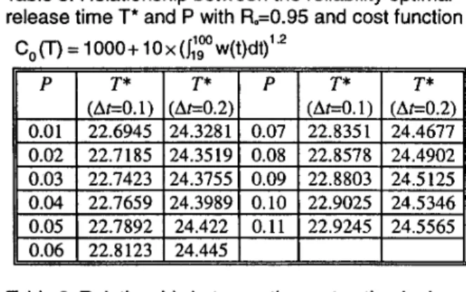
4.2.1. Numerical Example 2. Tables 3 shows the relationships between the reliability optimal release time T I * , At and P based on R,,= 0.95. From Tables 3, we find that as P increases, the optimal release time TI* increases. The reason is as follows. From Eq. (14), we know that R(At1T) denotes the conditional reliability function that the software will still operate after T+At given that it has not failed after time

T

[5-61. In addition, from Eq. (8), we know rn,(t)=(l+P)rn(t). That is, me(T +At)

-

me(T) = (1

+

P ) x

the reliability optimal release time. In fact, through new automated techniques/tools, it is probably easier to find these extra latent faults in the interval ( T I , Tl+At]. Therefore, the reliability optimal release time will be delayed till the reliability goal is reached.

Table

3:

Relationship between the reliability optimal release time T,* and P based on the first measure of software reliabjlity R.=0.95.

l P l T I *

I

TI*

I

P

I

TI*

I

TI*

4.3. Software release time based

on

cost-reliability

criterion considering efficiency

From subsection 4.2, we can easily get the required testing time needed to reach the reliability objective R,. Here our goal is to minimize the total software cost to achieve the desired software reliability and then the optimal software release time is obtained. Therefore, the optimal release policy problem can be formulated as minimizing C ( T ) , subject to R(AtlT)>R, where O<R,cl., i.e.,

r* = optimal software release time = mux(T, , T I )

where T,,= finite and unique solution T satisfying Eq. (13), and TI= finite and unique T satisfying Eq. (14), or Eq. (15). Combining the cost and reliability requirements and considering the efficiency, we have the following theorem.

Theorem

1:

Assume C o ( T ) = CO, +CO x

(I;

w(t)dr)" ,CoI>O, CaO, CpO, C2>0, C3>0, and C2>Cl, we have

(1)if u r x ( C , -C, ) e x p [ - r ( W ( T s ) - W ( 0 ) ) ] > C ~ andP(T&

<e3,

T

'

= max(T,, T I ) for R(A tlTs)<Ra<l or r'=T, for

O<R,

I

R(A AT,).

*

(6)

R(ArIT,)cRo<l or T'=T, for OCR,< R(AtlT,).

(3) if P(T&C,,

T

'

2T,

for R(ArIT,)cR,<I or

T'2

T, for O & , I R(AtlT,).

0.04

0.05 0.06

From the above theorem, we can easily determine the optimal software release time based on the cost and reliability requirements considering efficiency. Table 5 shows the cost-reliability optimal release time under different R,, At, and cost function. Similarly, Table 6 shows the relationship between the optimal release time T,

*

based on the target reliability R,(T) and l? From these tables and following the same arguments in Theorem 1, we can obtain the optimal software release time based on the cost and reliability criteria.

0.925 22.4203 0.10 0.982 27.2990 0.930 20.7667 0.11 0.991 27.6343 0.945 24.3389

R2(T)

I

5. Conclusions

In this paper we present an SRGM with generalized testing-effort function. It is a much more realistic model and more suitable for describing the software fault detectionhemoval process. Furthermore, we also discussed the effects of introducing new toolsltechniques for increased software testing efficiency, and studied the related optimal software release time problem from the cost- reliability viewpoint. The procedure for determining the optimal release time T* has been developed and the optimal release time has been shown to be finite. In practice, sometimes it is difficult for us to locate the faults that have caused the failure based on the test data reported in the test log and test anomaly documents. Therefore, it is advisable

to introduce, new toolsltechniques, which are fundamentally different from the methods in use. In addition, there are still many more potential cost functions. We will present further investigations on describing the mathematical properties of the SRGM with generalized testing-effort function in the future.

Acknowledgment

We would like to express our gratitude for the support of the National Science Council, Taiwan, R.O.C., under Grant NSC 87-TPC-E-002-017. Partial support of this work (by Michael R. Lyu) is provided by a UGC direct grant at CUHK. Referees' insightful comments and suggestions are also highly appreciated.

References

[l] S . Yamada, J. Hishitani, and S. Osaki, "Software Reliability Growth Model with Weibull Testing Effort: A Model and Application," IEEE Trans. on Reliability, Vol. R-42, pp. [2] S . Yamada and S . Osaki, " Cost-Reliability Optimal Release

Policies for Software Systems," IEEE Trans. on Reliability, Vol. 34, No. 5, pp. 422-424, 1985.

[3] J. D. Musa (1998). Sojiware Reliability Engineering: More Reliable Software, Faster Development and Testing. McGraw-Hill.

[4] C. Y. Huang, J. H. La and S . Y. Kuo, "A Pragmatic Study of Parametric Decomposition Models for Estimating Software Reliability Growth," Proceedings of the 9th Inrernational Symposium on Sofmare Reliability Engineering (ISSRE98),

pp. 11 1-123, Nov. 4-7. 1998, Paderbom, Germany. [SI C. Y. Huang, S . Y. Kuo and I. Y. Chen, "Analysis of a

Software Reliability Growth Model with Logistic Testing- Effort Function," Proceedings of the 8th International Symposium on Software Reliability Engineering (ISSRE97). pp. 378-388, Nov. 1997, Albuquerque, New Mexico. U.S.A. [6] K. Okumoto and A. L. Goel, "Optimum Release Time for

Software Systems Based on Reliability and Cost Criteria," Journal of Systems and Sojiware, Vol. 1, pp. 315-318, 1980. [7] M. R. Lyu (1996). Handbook of Sofhvare Reliability

Engineering. McGraw Hill.

[SI F. N. Parr, "An Alternative to the Rayleigh Curve for Software Development Effort," IEEE Trans. on Software Engineering, SE-6, pp. 291-296, 1980.

[9] M. Lipow, "Prediction of Software Failures," Journal of Systems and Software, Vol. 1, pp. 71-75, 1979.

[lo] M. Ohba, " Software Reliability Analysis Models," IBM J.

Res. Develop., Vol. 28, No. 4, pp. 428-443, July 1984. [I 11 J. Farquhar and A. Mosleh, "An Approach to Quantifying

Reliability-Growth Effectiveness," Proceedings Annual Reli- ability and Maintainability Symposium, pp. 166-173, 1995. [12] P. K. Kapur and R. B. Garg, "Cost-Reliability Optimum

Release Policies for a Software System under Penalty Cost," Int. J. of Systems Science, Vol. 20, pp. 2547-2562, 1989. [13] M. R. Lyu and A. Nikora, "Using Software Reliability

Models More Effectively," IEEE Software, pp. 43-52, 1992. 100-105, 1993.