Efficient and Exact Reliability Evaluation for
Networks With Imperfect Vertices
Sy-Yen Kuo, Fellow, IEEE, Fu-Min Yeh, and Hung-Yau Lin
Abstract—The factoring theorem, and BDD-based algorithms have been shown to be efficient reliability evaluation methods for networks with perfectly reliable vertices. However, the vertices, and the links of a network may fail in the real world. Imperfect vertices can be factored like links, but the complexity increases exponentially with their number. Exact algorithms based on the factoring theorem can therefore induce great overhead if vertex failures are taken into account. To solve the problem, a set of exact algorithms is presented to deal with vertex failures with little additional overhead. The algorithms can be used to solve terminal-pair, -terminal, and all-terminal reliability problems in directed, and undirected networks. The essential variable is defined to be a vertex or a link of a network whose failure has the dominating effect on network reliability. The algorithms are so efficient that it takes less than 1.2 seconds on a 1.67 GHz personal computer to identify the essential variable of a network having
299 paths. When vertex failures in a 3 10 mesh network are taken into account, the proposed algorithms can induce as little as about 0.3% of runtime overhead, while the best result from factoring algorithms incurs about 300% overhead.
Index Terms—BDD (Binary Decision Diagrams), Boolean for-mula, exact algorithm, network reliability.
DEFINITIONS
link network a network in which vertices are perfectly reliable, and only links may fail.
ordinary network a network in which vertices as well as links may fail. A network can be regarded as a link network, or an ordinary network depending on vertices being perfect or not.
Manuscript received May 8, 2006; revised December 15, 2006; accepted Jan-uary 31, 2007. This work was supported by Grant NSC 95-2221-E-002-068 by the National Science Council, Taiwan, and Grant 95R0062-AE00-05 by the Ex-cellent Research Projects, National Taiwan University. Associate Editor: R. H. Yeh.
S.-Y. Kuo is with the Department of Electrical Engineering, National Taiwan University, Taipei 106, Taiwan, and also with the Department of Computer Sci-ence and Information Engineering, National Taiwan University of SciSci-ence and Technology, Taipei, Taiwan (e-mail: [email protected]).
F.-M. Yeh is with the Department of Electrical Engineering, National Taiwan University, Taipei 106, Taiwan, and also with Gemtek Technology Co., Ltd., Hsinchu, Taiwan.
H.-Y. Lin is with the Department of Electrical Engineering, National Taiwan University, Taipei 106, Taiwan, and also with Advantech Co., Ltd., Taipei, Taiwan.
Color versions of one or more of the figures in this paper are available online at http://ieeexplore.ieee.org.
Digital Object Identifier 10.1109/TR.2007.896770
variable a variable is a link or a vertex. essential variable a variable other than source or
sink vertices of a network, whose failure has the dominating effect on network reliability.
inverted edge an edge in a BDD; and the binary value at the terminal node of a BDD is complemented if an inverted edge is followed.
overhead the time penalty incurred when perfect vertices in a network are treated as imperfect.
NOTATIONS vertex . link .
a Boolean variable which can represent a link , or a vertex .
an undirected link connecting vertex , and .
a directed link connecting from vertex to .
the success probability of a variable . a network graph with vertex set , and link set . Variable failures are statistically independent.
the number of elements in set . a specified subset of two or more vertices
in , i.e. , .
, i.e. the number of vertices in . a new graph derived from graph by contracting/deleting link .
a sub-graph of generated by moving to after all links connected to are deleted.
a -terminal ordinary network, or a terminal-pair ordinary network with source vertex , and sink vertex . The subscripts are optional and can be missing.
positive/negative cofactor of a Boolean
function , and they are derived by setting the Boolean variable in to 1 or 0 respectively.
Boolean AND/OR operation.
ACRONYM1
BDD reduced ordered binary decision diagrams [1].
the BDD representation of the reliability expression for network .
the -terminal reliability of . It is sometimes abbreviated as . BFS/DFS breadth-first/depth-first search. CAE/CAEK CAE (composition after expansion)
algorithm computes by taking imperfect vertices into account after graph expansion. CAEK is the
-terminal version of CAE.
EE/EEK EE (entangled expansion) algorithm computes by taking imperfect vertices into account during graph expansion. EEK is EE extended to solve
-terminal networks.
I. INTRODUCTION
L
ET be the specified subset of the vertices in a graph with . The -terminal reliability is the probability that the vertices in are con-nected. is called the all-terminal reliability, and is known as the terminal-pair reliability. Terminal-pair reliability is an important performance measure in communi-cation networks that use flooding for route setup, or packet transmission. The problem of computing for a generallink network has been studied for decades [2]. It was shown to
be NP-hard [3] in 1986 [4]. In the real world, the vertices, as well as the links of a network may fail. Taking into account the effect of imperfect vertices can only exacerbate the perfor-mance.
Many algorithms including exact, and approximation al-gorithms have been presented to solve network reliability problems [5]–[30]. Some algorithms require the minimal
paths/cuts to be enumerated in advance, and then the minimal
paths/cuts are manipulated to get their counterparts in the SDP (sum of disjoint product) form [15]–[18]. Cuts have been used to compute network reliability since the 1960s [6]. In many practical systems, the number of cuts is much smaller than the number of paths [19]. It was shown that cut-based algorithms often have better performance than path-based ones for some networks [20]. Nevertheless, the number of minimal paths/cuts in link networks still grows exponentially with the size of net-works. Enumerating minimal paths/cuts in a large link network quickly becomes impractical, even without measuring the effect of imperfect vertices in its counterpart ordinary network.
Some other algorithms are based on the factoring theorem [5], [12]–[14]. Moskowitz [5] was the first to employ the factoring theorem directly as a means of calculating network reliability. It is well known that, by using the factoring theorem, the reliability
1The singular and plural of an acronym are always spelled the same.
of a graph can be expressed recursively as
. In other words, the reliability of a graph can be expressed recursively by two smaller graphs. One graph has one fewer vertex, and one fewer link, while the other has only one fewer link. This method could be a pure numerical computation without the need to enumerate or store minimal paths or cuts. It was proved that the optimal binary structure of the factoring algorithm for undi-rected link networks can be generated by means of pivoting, and series-parallel probability reduction when links fail indepen-dently [10]. It was shown that the factoring theorem, combined with some reduction techniques such as the polygon-to-chain
re-duction, or the series-parallel rere-duction, can have good
perfor-mance for link networks [9], [12]–[14]. Imperfect vertices can be taken into account by factoring on links as well as on vertices. Unfortunately, this increases the complexity exponentially with the number of imperfect vertices, and renders the approach less attractive.
To deal with vertex failures, the most commonly used method is known as the incident edge substitution [21]. The method can be embedded in any algorithm that generates a symbolic reli-ability expression for link networks [8], [14], [21]. It expands each term of the reliability function derived for a link network by replacing the link variables with functions of vertex & link vari-ables. Boolean simplification is needed after the replacement. Unfortunately, the cost of these operations grows exponentially with the number of links. Furthermore, the required storage is prohibitively large if the symbolic expression rather than direct numerical computation is used [14]. A more feasible approach is to slightly modify the probability function used in the fac-toring theorem, and factor on links that have at least one per-fect endpoint [14]. The algorithm must exclude some reduction strategies for correct computation. It is well known that the ef-ficiency of a factoring algorithm relies on reduction strategies. The exclusion of some reduction strategies results in higher run-time overhead.
The algorithm in [23] tried a different approach by trans-forming an undirected network into a directed network. The re-liability was then obtained from the transformed network. It is an approximation algorithm, and also an exact algorithm if it is run to completion. The algorithm may be able to generate results with acceptable error within reasonable time, but it has been shown to generate incorrect results for some networks [24]. An-other brute-force algorithm using the path function, also known as the path-based reliability function, was proposed in [25].
The algorithms discussed above are not efficient for the fol-lowing reasons. 1) It is inefficient to derive SDP forms of com-plex Boolean functions. 2) The tree-based partitioning algo-rithms may not make use of isomorphic sub-graphs. Therefore, redundant computation may not be avoided. 3) It takes prohibi-tively large storage space to store the success/failure events of an event tree derived from a large network because the information of common variables in the events are not shared. 4) Most algo-rithms do not store the prohibitively large amount of informa-tion in a reliability expression or success/failure events so that they have to re-decompose the network graph when the proba-bilities of a few variables are changed. This makes the search for the essential variable inefficient. 5) No efficient method is
presented to handle the incident edge substitution, and the sub-sequent Boolean simplification.
It has been shown in [26]–[28] that reliabilities for link networks can be computed very efficiently by constructing the symbolic reliability functions with BDD. To compute the relia-bilities for ordinary networks, this paper presents two efficient exact algorithms, known as EE (entangled expansion), and CAE (composition after expansion). Both algorithms combine the simplicity of the incident edge substitution, and the merits of BDD. Both algorithms can be used to solve -terminal reliability problems, where can be any integer value from 2 to . Different from some other algorithms which can only handle directed networks, the proposed algorithm can handle directed, and undirected networks without the need of any network transformation. A very efficient method incorporating the CAE algorithm, and the BDD composition operation is also presented in this paper to identify the essential variable. The proposed algorithms are so efficient that 1) it takes the CAE algorithm 1.112 seconds on a 1.67 GHz personal computer to identify the essential variable of an ordinary network having paths, and 2) the CAE algorithm can induce less than 0.3% of runtime overhead when vertex failures in a 3 10 mesh network are taken into account. By contrast, the best result from factoring algorithms incurs about 300% of runtime overhead for the same mesh network [14].
Compared to previous algorithms, the proposed algorithms have the following advantages. 1) BDD can be very efficient in deriving SDP forms of complex Boolean functions. 2) Iso-morphic sub-graphs are reused in the network decomposition process by means of the edge expansion diagrams (EED) [27]. 3) Information of common variables can be shared in BDD. Due to the compact size of BDD, it is therefore possible to store the reliability expression of a large network in the form of a BDD in main memory or on disk. 4) The essential variable can be identi-fied with high efficiency by repeatedly substituting different nu-merical values for link/vertex variables into the stored reliability expression in main memory. 5) The incident edge substitution, and the subsequent Boolean simplification can be handled very efficiently by making use of BDD.
In the next section, readers are briefed on BDD basics. The proposed algorithms are presented in Section III. To be more specific, the proposed EE, and CAE algorithms are described in Sections III-A, and III-B respectively. In Section III-C, it then proceeds to the discussion of the algorithm for identifying the essential variable. The EE, and CAE algorithms are extended to solve -terminal reliability problems in Section III-D. The experimental results are tabulated and discussed in Section IV. Finally, the conclusions are drawn in Section V. Please note that BDD are used to perform all Boolean operations in this paper.
II. BDD BASICS
A. The Basics
The abbreviation BDD denotes a data structure for repre-senting Boolean functions, and an associated set of manipu-lation algorithms [1], [31]. Boolean functions are represented by directed acyclic graphs with restriction on the ordering of decision variables in the graph. In addition to the well-known
Shannon expansion, the BDD representation can also be ex-plained with the If-Then-Else (ITE) connective [32] for easier comprehension:
(1) where is a Boolean decision variable. Suppose , and are Boolean functions. If , and are two variables with a variable
ordering (refer to Section II-B) , the following equalities hold for the operations between two ITE connectives:
(2) The composition operation is an important BDD operation [1] used extensively in this paper. It constructs the graph for the function obtained by composing two functions, e.g. , and , below. This operation facilitates the incident edge substitution in a reliability expression. According to the following expan-sion, composition can be expressed in terms of cofactors, and Boolean operations, derived directly from the Shannon expan-sion.
(3) In this paper, a solid (respectively dashed) line in a BDD represents a BDD node taking the value 1 (respectively 0). A Boolean function , and its complement , are identical except that their two terminal nodes, TRUE, and FALSE, are swapped. This property can be exploited by using inverted edges in BDD representations. With inverted edges, only one constant node is needed. By using inverted edges, the size of a BDD can be reduced, and the performance can also be improved at the same time [31], [33]. For the twelve examples used in [31], the BDD representations with inverted edges were 7% smaller than those without using them. Furthermore, the execution time is decreased by almost a factor of 2. Although inverted edges were used in our experiments, they were not drawn in the illustrative figures.
B. Variable Orderings
A particular sequence of variables in BDD is known as a variable ordering. BDD in a given variable ordering will be in
canonical forms, i.e. every function has a unique representation,
after applying the elimination, and mergence rules. The
elimina-tion rule is to eliminate a node whose positive cofactor, and
neg-ative cofactor are connected to the same graph. The mergence
edges of these graphs to the merged graph. Two functions are equivalent iff they are isomorphic BDD graphs in the same vari-able ordering.
The efficiency of BDD manipulation operations is determined by the size, i.e. the number of nodes, in a BDD. It has been ob-served that the size of a BDD depends on variable orderings. As a dramatic example, the BDD of a multiplexer with vari-ables has less than nodes in the best variable ordering, while it has more than nodes in the worst variable ordering. A variable ordering for a function is described as a good one if a compact BDD graph of the function can be generated in that ordering. The optimal variable ordering, defined in the same sense, can generate the most compact BDD. Although an al-gorithm of time complexity was presented to find the optimal variable ordering [34], it is not practical for real world applications. Furthermore, it has been shown that improving the variable ordering of BDD is NP-complete [35]. Fortunately, the BFS or DFS from source vertex to sink vertex seems to usually generate variable orderings good enough for applications of net-work reliability computation [26], [27].
III. THEPROPOSEDALGORITHMS
This section begins with the discussion of the network de-composition technique presented in [27]. Then, we show how to take imperfect vertices into account in each step of the net-work decomposition process by making intuitive modifications to the technique in [27]. The strategy EE (entangled expansion), along with an example, is given. A generally faster algorithm CAE (composition after expansion), making use of the incident edge substitution, is presented in the subsequent section with an illustrative example. These two algorithms are then extended to handle -terminal networks. Although the ITE connectives are used in this section, BDD operations shall take the place of all Boolean operations in a computer program.
A. Entangled Expansion
It was shown that BDD, combined with edge expansion dia-grams, is an efficient way to construct symbolic reliability ex-pressions, and to calculate the reliability value for link networks [26]–[28]. The edge expansion diagram is a recursive network decomposition method, which is similar to but different from the contraction operation of the factoring theorem. Suppose is a graph with source vertex , and the links emitted from
are or . The sub-graphs of
gen-erated by edge expansion diagrams are denoted by , which is the result of moving to after all links connected with are deleted. On the contrary, the contraction operation in the factoring theorem keeps all links except . The symbolic reliability expression for link network can be expressed
re-cursively as , where performs
Boolean summation. All paths are implicitly encoded into the BDD of even though they are not enumerated. This is the basic idea of the EED algorithm in [27]. However, for data to flow from to through in ordinary network , all these three variables have to be successful. It is clear that the sym-bolic reliability expression for ordinary network can be
ex-pressed recursively as , or
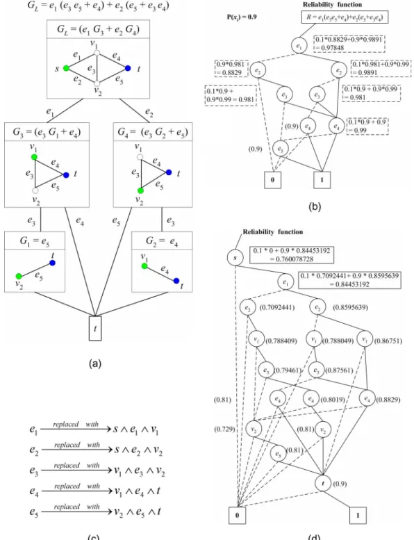
Fig. 1. Entangled expansion. (a) Edge expansion diagram; (b) reliability ex-pression.
, depending on being directed, or undirected respectively. This technique, as demon-strated in Fig. 1(a) & the ITE form below, is named EE.
As soon as the reliability expression of was encoded in a BDD, the reliability value can be easily calculated by traversing the BDD. This process can be expressed recursively with (4), where is the top variable of .
(4)
Fig. 1(a) is deliberately chosen because it is simple enough to illustrate the BDD operations with the ITE connectives. Any Boolean variable can be written in ITE form, as shown in (5). Because the derivations below contain many levels of parentheses, the ITE form is also written in a way similar to a three-row column matrix for easier comprehension. The first row is the variable name; and the second row, and third row are the function or constant when the variable takes TRUE, and FALSE respectively.
(5)
Suppose the variable ordering is
. With the help of edge expansion diagrams, the reliability expression of Fig. 1(a) can be derived with entangled expansion, as in (6) at the bottom of the next page.
It can be checked that (6) maps gracefully to Fig. 1(b). Both , and nodes in the left of Fig. 1(b) have two incoming lines. The four incoming lines of , and map to the double
oc-currences of , and in (6).
In other words, the ITE form does not make use of isomor-phic terms or graphs, while the BDD does. Please note that the phrase “isomorphic graphs” is used both in BDD, and in edge expansion diagrams to represent different ideas. Only one of the
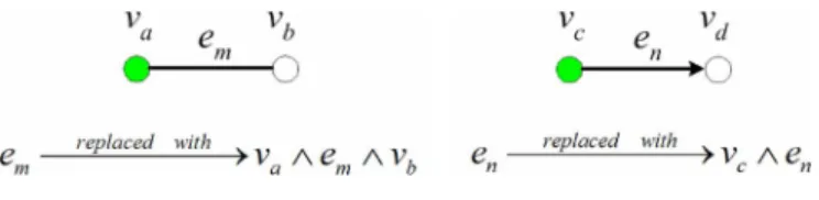
Fig. 2. Incident edge substitution.
isomorphic graphs in edge expansion diagrams needs to be de-composed. The isomorphic graphs in BDD are not to be decom-posed, but rather encode some information.
B. Composition After Expansion
Whenever a logic operation requires a link in the entangled expansion, its two endpoints are taken into account. This method is simple, and effective. However, the , and operations which once involved a link variable in one of the arguments now re-quires at most three variables rather than just one. Many sub-graphs may be decomposed on the same link more than once. For many networks, this may slow the algorithm slightly. An-other strategy, named CAE, making use of the BDD composi-tion operacomposi-tion is therefore suggested. The strategy is just another incarnation of the incident edge substitution. The incident edge substitution is based on a simple concept: the failure of a vertex
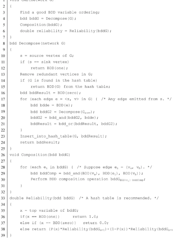
Fig. 3. Pseudocode for the CAE algorithm.
implies the failures of its incident links. Suppose , and . According to the concept, , and in the reliability expression are replaced with , and
respectively, as illustrated in Fig. 2.
Even though incident edge substitution can be embedded into any symbolic reliability expression of link networks, no efficient algorithm was presented to deal with the subsequent Boolean simplification. Fortunately, the substitution, and the subsequent Boolean simplification can be facilitated by the BDD
composi-tion operacomposi-tion if the reliability expression of a link network is encoded with BDD in advance. The composition operation can be performed with (7), or (8) depending on the link being undi-rected, or diundi-rected, respectively.
Fig. 4. An example for the CAE algorithm. (a) Edge expansion diagram; (b)BDD(G ); (c) substitution function; (d) BDD(G ).
(8) CAE can be used to calculate the terminal-pair reliability of an ordinary network. The pseudo-code of CAE in the C programming language style is listed in Fig. 3. The first step is to generate a good BDD variable ordering with a heuristic algorithm such as the BFS. The BDD of graph is decomposed with the edge expansion diagram [27] as if all the vertices are perfect. The composition operation is then used to perform the incident edge substitution, and this generates the BDD of the
reliability expression for graph . Finally, the BDD of is traversed once to calculate the network reliability. A hash table can greatly improve the performance of the reliability calcula-tion, and it is recommended for the function in Fig. 3. The pseudo-code in Fig. 3 is for undirected graphs. For directed graphs, the code in line 29 needs to be changed
from “ a i b ;”
to “ c j ;”.
Fur-thermore, the code in line 12 needs to be changed from
“ ;” to “ ;” because the sink
The EE algorithm can also be implemented with slight modi-fications to the pseudo-code in Fig. 3. First, the
function is deleted. Then, the code in line 18 is changed to
“ a i b ;” for
undi-rected graphs, or “ c i ;”
for directed graphs. Because the sink vertex is imperfect, the code in line 12 needs to be replaced with “ ;”.
The ITE form of the CAE algorithm for Fig. 1 can be easily derived. First, derive the ITE form of with the same variable
ordering used above, i.e. .
(9)
Then, the composition operation in (7) is applied to (9) to re-place link variables with their incident edge functions. With some ITE manipulations, it can be checked with ease that the result of the composition operation will be the same as that in (6).
Fig. 4 is another example illustrating the CAE algorithm. The success probabilities of all variables are assumed to be 0.9. First, the BDD of is constructed. Then, all link variables in Fig. 4(b) are replaced with the substitution function in Fig. 4(c) by using the BDD composition operation. This results in the BDD in Fig. 4(d). The derivation of the ITE form of this ex-ample is too lengthy, and it is not shown here without the loss of generality. Finally, the reliability value, which is about 0.76, can be calculated by traversing the BDD in Fig. 4(d).
C. The Essential Variable
In the design of a network topology, it is important to identify the most crucial component of a network so that efforts can be made to keep it functional. The essential variable is defined with (10) to help identify the most crucial component.
(10) In other words, an essential variable of a network is either a link, or a vertex other than the source or sink ver-tices, whose failure has the dominating effect on network reli-ability. To search for the essential variable, it can be assumed that each variable in fails in turn in a loop, and is removed from the graph. A new graph is there-fore created in one iteration of the loop, and the new graph can be solved with the CAE algorithm. Please note that many iso-morphic sub-graphs may be generated inside the loop. The hash table for isomorphic graphs can therefore be reused. The perfor-mance of this intuitive method is better than repeatedly starting and terminating the CAE program without hash table reuse. The pseudo-code for this intuitive method is only two lines.
for (each variable xi other than s and t in GN;(2))
CAE (GN;(2)0 xi);
The minimum reliability value, and therefore the essential variable, can be determined after the loop. Although the intu-itive method above can generate correct results, it wastes time in redundant operations because the CAE algorithm is called many times. Each invocation of the CAE algorithm decomposes a network. Another better approach is to make use of the BDD composition operation to its full potential. First, the BDD of the graph is constructed. Then, each variable in is substituted in turn with BDD(zero) in each iteration of a loop. This operation generates the BDD of without re-peatedly decomposing the networks . The BDD of can then be traversed to calculate the reliability. In this way, needs only to be decomposed once. Be-cause the BDD composition operation is very efficient, it makes this approach highly efficient. The pseudo-code of the proposed method is listed below.
Construct BDD(GN;(2));
for (each variable xi other than s and t in GN;(2)) {
BDD(GN;(2)0 xi) = BDD(GN;(2))jxi=0;
Reliability(BDD(GN;(2)0 xi));
}
For example, consider the network at the top of Fig. 4(a). There are four vertices, and five links in the graph . To identify the essential variable, the intuitive method assumes that each variable in fails in turn, and is removed from the original graph. Seven network graphs will be created. Similar to the process in Fig. 4(a)–(4d), each of the seven graphs is solved with the CAE algorithm. This means that each of the seven graphs is decomposed once. This method can be expressed as . This method wastes precious time in redundant computations. The much better method discussed above makes use of the BDD composition operation to its full potential. Firstly, the reliability expression of the original ordinary network graph is encoded in a BDD in the way identical to Fig. 4(a)–(4d). Secondly, in the BDD in Fig. 4(d), each of the seven variables in is assumed to take the 0-edge in turn. This process creates seven BDD without decomposing any other network graph. Finally, the seven BDD are then traversed to calculate their reliability values. This method can be expressed as . The essential variable can thus be identified. The essential variables of the network are
, and because ,
, and .
D. Extension to -Terminal Networks
The EE & CAE algorithms can be easily extended to handle -terminal networks by decomposing networks with the con-traction operation. The concon-traction operation keeps all links
TABLE I
BENCHMARKRESULTS FORTERMINAL-PAIRNETWORKS
Network 1: Example 11 in [14], Network 2: Example 6 in [14], Network 3: Example 8 in [14], Network 6: Figure 1 in [14] 0: time value less than 0.001
-: not available
connected with the source vertex, except that the link being contracted is deleted. This may result in many parallel links. The parallel links can be removed in terminal-pair networks, but they have to be kept in -terminal networks. This simple strategy is known as the brute-force algorithm, for it is less effi-cient. Another strategy is to pick pairs of terminal vertices from the terminal vertices, derive the terminal-pair reliability expression for these terminal pairs, and perform Boolean AND operation on these reliability expressions. These terminal pairs must include all the vertices in . It may not be a good idea to pick the terminal pairs at random. Many sub-graphs may be generated during the decomposition process of each of the terminal-pair networks. The performance will be improved if redundant decomposition can be avoided by making use of the intermediate isomorphic sub-graphs. This is the main idea of the fixed-sink algorithm [28]. In the fixed-sink algorithm, one of the vertices in is chosen as the terminal vertex, and each of the remaining vertices is regarded in turn as the source vertex so that terminal-pair networks are created. Suppose . To solve the -terminal network reliability problem, the pseudo-code in the forth line of Fig. 3 shall be replaced with the following pseudo-code statement.
v1vk
v2vk vk 1vk
Both EE & CAE algorithms can be extended to solve -ter-minal ordinary networks by incorporating the strategy of the fixed-sink algorithm, and their -terminal counterparts are re-ferred to as EEK & CAEK respectively in this paper. Take the network graph at the top of Fig. 4(a) as an example. Let
. Because is equal to three, two terminal pairs must be selected to include all elements in . In a -terminal net-work, any vertex can be the fixed sink. Let be chosen as the fixed sink. Then, the two terminal pairs are , and .
The BDD of the reliability expression for the 3-terminal net-work can be constructed by the pseudo-code below.
s v1 t v1
IV. EXPERIMENTALRESULTS
The proposed algorithms were implemented in the C++ pro-gramming language for comparison with existing results in the literature. Instead of using an integer for each link, the bit vector representation of links was used to store information of network topologies. This technique could speed up the search for the iso-morphic graphs in the hash table. The CMU BDD library [36] was used to handle the BDD operations. All the program files were compiled with GNU g ++ 4.1.0, and the optimization flag was used. The CPU time in seconds was measured with the timecommand on a personal computer, which contained 1 GB of memory, and a single AMD Athlon-XP processor (with 256 KB L2 cache) running at 1.67 GHz. The operating system was a Linux system with kernel version 2.6.16. The variable ordering algorithm used in this section is almost the same as the BFS al-gorithm in [26], except that the end points of a link were given an ordering as soon as the link is ordered.
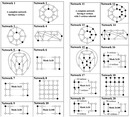
The algorithm presented in [14] was the most efficient algo-rithm capable of handling large ordinary networks, and it was compared to the proposed algorithms, EE, and CAE. The bench-mark networks in Fig. 5 were used, and the results were listed in Table I, and Table II. All nodes, and links variables have the same success probability of 0.9. Networks 1–10 are ter-minal-pair networks, and Networks 11–20 are -terminal net-works in which is about . The main reason for using these networks in the experiments is that they have been used in the literature. Therefore, experimental results from other papers can be used for comparison or verification. Many other network topologies have been benchmarked in our experiments. How-ever, those results are not listed in this paper simply because of the space limitation.
Fig. 5. Benchmark networks.
Without the composition operation, the CAE algorithm can degenerate into the EED algorithm [27], which can be used to calculate terminal-pair reliability for link networks. The degen-erated CAE algorithm is labeled as EED in Table I. The EED & CAE algorithms finished their execution so fast that small dif-ference in time value could contribute one or two percentages to the overhead. Each program was run 10 times, and the average value was used. Larger networks are more immune to the impre-cision of time measurement. The degenerated CAE algorithm, i.e. EED, is 1688 times faster than the result in [14] for link Net-work 6, while CAE is 6775 times faster than the result in [14] for ordinary Network 6. The CAE algorithm incurs less than 0.3% of runtime overhead if the imperfect vertices are considered. By contrast, the result
in [14] induced 300% of
runtime overhead. The machine used in [14] was the VAX 8530. Even if the CPU speed difference is considered, the proposed al-gorithms still have speed advantage. Furthermore, the proposed algorithms have another merit. They are able to decompose a network once, store its reliability expression in BDD, and the BDD can then be reused to compute network reliabilities with different variable probability values. This property also makes the identification of essential variables of a large network highly efficient.
One of the attractive BDD properties is that the reliability ex-pression of a network is canonical for a given variable ordering. The correctness of different implementation can be verified by checking whether two BDD-based reliability expressions are equivalent or not. The EE, and CAE algorithms were verified
to generate equivalent BDD for the benchmark networks. The column Nodes in Table I & Table II lists the number of BDD nodes in the reliability expression. Each BDD node takes only 16 bytes of main memory space in our 32-bit machine. The re-liability function of Network 5 contained 15,795 BDD nodes, which occupied less than 272 KB of main memory space. From the results in these tables, it is clear that the proposed algorithms are very efficient in terms of speed, and memory space.
Table III lists the results of the essential variable analysis, which makes use of the BDD composition operation discussed in Section III-C. The column Essential lists the reliability value when the essential variable fails. The value is defined to be the lowest reliability when one of the variables other than or fails, and it is referred to as the essential reliability later in this paper. The column Average, defined with (11), is the average reliability value of a network when each variable other than or in the network fails in turn. The column Sensitivity is defined with (12).
(11)
(12)
From the results in Tables I–III, Network 1 has the most reli-able topology. However, the higher reliability comes at the cost of more interconnection links, and this may result in a more ex-pensive network. On the other hand, the long, thin mesh net-works, such as Network 9 & 10, have lower reliability value,
TABLE II
BENCHMARKRESULTS FORk-TERMINALNETWORKS
TABLE III
ESSENTIALVARIABLEANALYSIS
and higher sensitivity. If the leftmost two vertices of Network 9 are connected to the rightmost two vertices, the network will be-come an annular network similar to Network 2. Although only two links are added to Network 9, the network becomes much more reliable, and failure resistant. The reliability value will be increased from 0.23016 to 0.779331, and the sensitivity will drop from 0.218321 to 0.0100386. Most important of all, the es-sential reliability will be increased from 0.139753 to 0.670082. In other words, the reliability value will always remain higher than 0.67, even if a component in the network fails. Networks 7 & 9 have roughly the same number of links & vertices. Net-work 7 is much more reliable, and less susceptive to component failures than Network 9 thanks to its better topology, and higher ratio of links to vertices.
The result in [14] demonstrated how the runtime overhead of considering imperfect vertices grows with mesh networks of size less than 3 10. The same type, but different size of mesh networks was tested in the experiments. The result is listed in Table IV. The table indicates that the CAE algorithm incurs lower runtime overhead than the EE algorithm, and much lower overhead than the algorithm in [14]. The CAE algorithm induces less than 0.3% overhead for all test cases in the table, and this is much better than any other published algorithms we know.
As discussed above, algorithms which require path/cut enu-meration are impractical for large networks because paths/cuts grow exponentially with the size of networks. The claim can be demonstrated by using the 3 12 mesh network as the input file to the cut-based algorithm in [30]. The cut-based algorithm took 34.442 seconds to finish, while the CAE algorithm took only 0.7172 second. The cut-based algorithm spent 27.978 sec-onds generating all the 34,241 cuts. That elapsed time is about 80% of the total time. The efficiency of the CAE algorithm lies on the fact that it does not enumerate all the paths of a network. Instead, it constructs the symbolic path-based reliability func-tion of a network implicitly with BDD.
V. CONCLUSIONS
Network reliability problems have been studied for decades. The assumption that vertices are perfectly reliable was often made when solving these problems. However, links as well as vertices can fail in the real world. Previous algorithms incur great overhead when vertices are considered to be imperfect. This paper presents two low overhead strategies, named EE, and CAE, to take imperfect vertices into account. Both strategies can be extended to solve -terminal reliability problems. The best result from previously published algorithms capable of dealing
TABLE IV RESULTS FORMESHNETWORKS
with imperfect vertices incur as high as 300% of runtime over-head for the 3 10 mesh network, while the CAE algorithm induces as low as 0.3% of runtime overhead for the same net-work. It is very important to be able to compute the reliability values when one of the components in a network fails so that the most critical component, also known as the essential variable, of a network topology design can be located. Network designers can therefore use higher quality components in the most critical locations, or design a network topology in which no single com-ponent failure can reduce the reliability under certain threshold value. A highly efficient algorithm is also presented to identify the most critical component. The high efficiency results from the fact that it reuses the encoded reliability expression, and de-composes a network only once. The algorithm is so efficient that it takes less than 1.2 seconds on a 1.67 GHz personal computer to identify the essential variable of a network having paths. All the algorithms presented in this paper can be applied to di-rected, and undirected networks.
Although the proposed algorithms are more efficient than any previous algorithms, the proposed algorithms have their own limitation. As with any other algorithm making use of BDD, the efficiency of the proposed algorithms depends on the se-lected BDD variable orderings. Even though the optimal vari-able ordering can be found by an exhaustive search algorithm of time complexity , the exhaustive search algorithm is not practical for most real world applications. This paper uses the BFS algorithm for finding a variable ordering which is good enough for the application. How to find a better variable or-dering, if there is any, for all or most of network topologies in a short period of time is the work of the future. Another future work is to derive the time complexity for the proposed algo-rithms.
REFERENCES
[1] R. E. Bryant, “Graph-based algorithms for Boolean function manipula-tion,” IEEE Trans. Computers, vol. 35, no. 8, pp. 677–691, Aug. 1986. [2] R. E. Barlow and F. Proschan, Mathematical Theory of Reliability. :
J. Wiley & Sons, 1965, (Reprinted 1996).
[3] M. R. Garey and D. S. Johnson, Computers and Intractability: A Guide
to the Theory of NP-Completeness. : W. H. Freeman, 1979. [4] M. O. Ball, “Computational complexity of network reliability analysis
an overview,” IEEE Trans. Reliability, vol. 35, no. 3, pp. 230–239, Aug. 1986.
[5] F. Moskowitz, “The analysis of redundancy networks,” AIEE Trans.
Communications and Electronics, vol. 39, pp. 627–632, 1958.
[6] P. A. Jensen and M. Bellmore, “An algorithm to determine the relia-bility of a complex system,” IEEE Trans. Reliarelia-bility, vol. 18, no. 4, pp. 169–174, Nov. 1969.
[7] L. Fratta and U. G. Montanari, “A Boolean algebra method for com-puting the terminal reliability in a communication network,” IEEE
Trans. Circuit Theory, vol. 20, no. 3, pp. 203–211, May 1973.
[8] L. Fratta and U. G. Montanari, “A recursive method based on case anal-ysis for computing network terminal reliability,” IEEE Trans.
Commu-nications, vol. 26, no. 8, pp. 1166–1177, Aug. 1978.
[9] M. Resende, “A program for reliability evaluation of undirected net-works via polygon-to-chain reductions,” IEEE Trans. Reliability, vol. 35, no. 1, pp. 24–29, Apr. 1986.
[10] A. Satyanarayana and M. K. Chang, “Network reliability and the fac-toring theorem,” Networks, vol. 13, pp. 107–120, 1983.
[11] A. Satyanarayana and R. K. Wood, “A linear-time algorithm for computingK-terminal reliability in series-parallel networks,” SIAM
J. Computing, pp. 818–832, 1985.
[12] L. Resende, “Implementation of a factoring algorithm for reliability evaluation of undirected networks,” IEEE Trans. Reliability, vol. 37, no. 5, pp. 462–468, Dec. 1988.
[13] L. B. Page and J. E. Perry, “Reliability of directed networks using the factoring theorem,” IEEE Trans. Reliability, vol. 38, no. 5, pp. 556–562, Dec. 1989.
[14] O. R. Theologou and J. G. Carlier, “Factoring & reductions for net-works with imperfect vertices,” IEEE Trans. Reliability, vol. 40, no. 2, pp. 210–217, Aug 1991.
[15] J. A. Buzacott, “The ordering of terms in cut-based recursive disjoint products,” IEEE Trans. Reliability, vol. 32, no. 5, pp. 472–474, Dec. 1983.
[16] K. D. Heidtmann, “Smaller sums of disjoint products by subproduct inversion,” IEEE Trans. Reliability, vol. 38, no. 3, pp. 305–311, Aug. 1989.
[17] J. M. Wilson, “An improved minimizing algorithm for sum of disjoint products,” IEEE Trans. Reliability, vol. 39, no. 1, pp. 42–45, Apr. 1990. [18] S. Soh and S. Rai, “Experimental results on preprocessing of path/cut terms in sum of disjoint products technique,” IEEE Trans. Reliability, vol. 42, no. 1, pp. 24–33, Mar. 1993.
[19] K. K. Aggarwal, Y. C. Chopra, and J. S. Bajwa, “Modification of cut-sets for reliability evaluation of communication systems,”
Microelec-tronics and Reliability, vol. 22, no. 3, pp. 337–340, 1982.
[20] Y. G. Chen and M. C. Yuang, “A cut-based method for terminal-pair reliability,” IEEE Trans. Reliability, vol. 45, no. 3, pp. 413–416, Sep. 1996.
[21] K. K. Aggarwal, J. S. Gupta, and K. B. Misra, “A simple method for evaluation of a communication system,” IEEE Trans. Communications, vol. 23, pp. 563–566, May 1975.
[22] W. J. Ke and S. D. Wang, “Reliability evaluation for distributed com-puting networks with imperfect nodes,” IEEE Trans. Reliability, vol. 46, no. 3, pp. 342–349, Sep. 1997.
[23] D. Torrieri, “Calculation of node-pair reliability in large networks with unreliable nodes,” IEEE Trans. Reliability, vol. 43, no. 3, pp. 375–377, Sep. 1994.
[24] Y. Chen, A. Q. Hu, K. W. Yip, X. Hu, and Z. G. Zhong, “A modified combined method for computing terminal-pair reliability in networks with unreliable nodes,” in Proceedings of the 2nd Int’l Conference on
[25] V. A. Netes and B. P. Filin, “Consideration of node failures in net-work-reliability calculation,” IEEE Trans. Reliability, vol. 45, no. 1, pp. 127–128, Mar. 1996.
[26] F.-M. Yeh and S.-Y. Kuo, “OBDD-based network reliability calcula-tion,” Electronics Letters, vol. 33, no. 9, pp. 759–760, Apr. 1997. [27] S. Y. Kuo, S. K. Lu, and F. M. Yeh, “Determining terminal-pair
network reliability based on edge expansion diagrams using OBDD,”
IEEE Trans. Reliability, vol. 48, no. 3, pp. 234–246, Sep. 1999.
[28] F. M. Yeh, S. K. Lu, and S. Y. Kuo, “OBDD-based evaluation of K-ter-minal network reliability,” IEEE Trans. Reliability, vol. 51, no. 4, pp. 443–451, Dec. 2002.
[29] F. M. Yeh, H. Y. Lin, and S. Y. Kuo, “Analyzing network reliability with imperfect nodes using OBDD,” in Proceedings of the 2002 Pacific
Rim Int’l Symposium on Dependable Computing (PRDC 2002), 2002,
pp. 89–96.
[30] H.-Y. Lin, S.-Y. Kuo, and F.-M. Yeh, “Minimal cutset enumeration and network reliability evaluation by recursive merge and BDD,” in
Proceedings of the 8th IEEE Int’l Symposium on Computers and Com-munication (ISCC 2003), 2003, pp. 1341–1346.
[31] K. S. Brace, R. L. Rudell, and R. E. Bryant, “Efficient implementation of an OBDD package,” in Proceedings of the 27th Design Automation
Conference, Jun 1990, pp. 40–45.
[32] W. S. Jung, S. H. Han, and J. Ha, “A fast BDD algorithm for large coherent fault trees analysis,” Reliability Engineering & System Safety, vol. 83, no. 3, pp. 369–374, Mar. 2004.
[33] S. I. Minato, N. Ishiura, and S. Yajima, “Shared binary decision dia-grams with attributed edges for efficient Boolean function manipula-tion,” in Proceedings of the 27th Design Automation Conference, Jun. 1990, pp. 52–57.
[34] S. J. Friedman and K. J. Supowit, “Finding optimal variable ordering for binary decision diagrams,” IEEE Trans. Computers, vol. 39, no. 5, pp. 710–713, May 1990.
[35] B. Bollig and I. Wegener, “Improving the variable ordering of OBDDs is NP-complete,” IEEE Trans. Computers, vol. 45, no. 9, pp. 993–1002, Sep. 1996.
[36] The BDD Library [Online]. Available: http://www-2.cs.cmu.edu/ afs/cs/project/modck/pub/www/bdd.html
Sy-Yen Kuo is a Chair Professor and Dean of the College of Electrical and Computer Engineering, National Taiwan University of Science and Technology, Taipei, Taiwan. He is also a Distinguished Professor at the Department of Elec-trical Engineering, National Taiwan University where he is currently on leave and was the Chairman at the same department from 2001 to 2004. He received the BS (1979) in Electrical Engineering from National Taiwan University, the MS (1982) in Electrical & Computer Engineering from the University of Cal-ifornia at Santa Barbara, and the PhD (1987) in Computer Science from the University of Illinois at Urbana-Champaign. He spent his sabbatical years as a Visiting Professor at the Computer Science and Engineering Department, the Chinese University of Hong Kong from 2004–2005, and as a visiting researcher at AT&T Labs-Research, New Jersey from 1999 to 2000, respectively. He was the Chairman of the Department of Computer Science and Information Engi-neering, National Dong Hwa University, Taiwan from 1995 to 1998, a faculty member in the Department of Electrical and Computer Engineering at the Uni-versity of Arizona from 1988 to 1991, and an engineer at Fairchild Semicon-ductor and Silvar-Lisco, both in California, from 1982 to 1984. In 1989, he also worked as a summer faculty fellow at the Jet Propulsion Laboratory of the Cali-fornia Institute of Technology. His current research interests include dependable systems and networks, software reliability engineering, mobile computing, and reliable sensor networks.
Professor Kuo is an IEEE Fellow. He has published more than 270 papers in journals and conferences. He received the distinguished research award between 1997, and 2005 consecutively from the National Science Council in Taiwan and is now a Research Fellow there. He was also a recipient of the Best Paper Award in the 1996 International Symposium on Software Reliability Engineering, the Best Paper Award in the simulation and test category at the 1986 IEEE/ACM Design Automation Conference (DAC), the National Science Foundation’s Re-search Initiation Award in 1989, and the IEEE/ACM Design Automation Schol-arship in 1990, and 1991.
Fu-Min Yeh received the B.S. degree in 1985 in electronic engineering from Chung-Yuan Christian University, the M.S. degree in 1992 in electrical engi-neering from National Taiwan University, and the Ph.D. degree in 1997 in elec-trical engineering from National Taiwan University. He was a deputy chief at the Electronic System Research Division of Chung-Shan Research Institute of Science and Technology from 1997 to 2006. He is the Director of the R&D Division II, Gemtek Technology Co., Ltd., Hsinchu, Taiwan. His research in-terests include wireless communication system, WiMax, UWB baseband de-sign, radar system dede-sign, hardware verification, VLSI testing, and fault-tolerant computing.
Hung-Yau Lin received in 1998 the B.S. degree in mechanical engineering from National Taiwan University, Taipei, Taiwan. He received his Ph.D. degree in electrical engineering from the same university in 2006. His research interests include computer graphics, data compression, memory repair algorithms, net-work reliability analysis, and computer operating systems. He is serving the duty of the Alternative Military Service for Defense Industry under a four-year contract as a senior engineer in Advantech Co., Ltd., Taipei, Taiwan.