行政院國家科學委員會專題研究計畫成果報告
國科會專題研究計畫成果報告撰寫格式說明
Preparation of NSC Project Reports
計畫編號:NSC 93-2115-M-009-011
執行期限:93 年 8 月 1 日至 94 年 7 月 31 日
主持人:陳秋媛 國立交通大學應用數學系
[email protected]
計畫參與人員:劉維展、藍國元、羅經凱、胡世謙
以上均為國立交通大學應用數學所研究生
一、中文摘要 本計劃之目的在於研究「雙環式網路」、 「三環式網路」、及「連接網路」。本計 劃為兩年期計劃,現為第一年,在這一年 中,我們的研究重點放在「退化的雙環式 網路」、「混合的弦環式網路」、以及「多 級式連接網路」上。 本計劃截至目為止,已經完成三篇論文(請 參看後面所附論文)。其中一篇是關於「雙 環式網路」、兩篇是關於「多級式連接網 路」。 在「雙環式網路」方面,我們探討當一個 雙環式網路的 L-shape 是 degenerate 時,參 數(l, h, p, n)的給法。在「多級式連接網路」 方面,我們研究 buddy networks with an arbitrary number of stages 的等價關係、以及 提 出 一 個 很 有 效 率 的 tag-based routing algorithm for the backward network of a bidirectional general shuffle-exchange network。關鍵詞:環式網路、雙環式網路、三環式 網路、連接網路、直徑
Abstract
The purpose of this project is to study loop networks and interconnection networks. This
its first year. In this year, we focus on the study of degenerate double-loop networks, the equivalence relation of buddy networks, and the routing algorithm for the backward network of a bidirectional shuffle-exchange network.
Keywords: loop network, double-loop
network, triple-loop network, interconnection network, diameter 二、緣由與目的 本人因旁聽黃光明教授之課程而對「環式 網路」產生很大之興趣,在過去幾年中, 所做的研究也以「環式網路」為主。然而, 由於「連接網路」在現今的研究及實際應 用中,都佔有極重要的地位,故想藉由此 計劃,對「環式網路」中的一些問題再做 研究,同時,也開始「連接網路」方面之 研究。 三、結果與討論 本計劃在第一年內,截至目為止,已經完 成了三篇論文:其中一篇論文已經投稿、 另外兩篇論文已經全部寫完了,最近就會 投稿;除此之外,還有幾篇論文正在撰寫 中。總之,今年是豐收的一年。以下略述 已完成的那三篇論文的結果。
論文一:Equivalence of buddy networks with arbitrary number of stages. [5]
網路個數。
在過去,學者們曾提出 buddy networks 及 strict buddy networks,也研究過 banyan 多 級式連接網路的等價關係(網路中的 stage 數都有所限制)。在這篇論文裡,我們推 廣 strict buddy networks 成 為 universal buddy networks、也推廣 P(*,*) networks 成 為 power-of-d networks。
由於 banyan 多級式連接網路是 universal buddy networks 的 special case,在這篇論 文裡,我們研究 universal buddy networks with an arbitrary number of stages 的等價關 係。
論文二:On degenerate double-loop L-shapes. [12] 論文[4]及論文[9]均曾提出一個「雙環式網 路」的L-shape是degenerate case時,參數(l, h, p, n)的給法。然而兩篇論文所給之參數 未必一致,論文二之目的即在討論兩者之 關係。 我 們 首 先 得 出 了 一 個 雙 環 式 網 路 的 L-shape 是 degenerate 的充分必要條件;接 著,我們證明了 L-shape 是 degenerate 時, 只會有 7 種可能的 shapes: (S1), (S2), …, (S7)。 為方便,稱論文[9]的參數(l, h, p, n) 的給法 為 CH-ALGO , 稱 論 文 [4] 的 給 法 為 CH-RULE。我們證明了:CH-ALGO 只會 得出(S1), (S2), (S3), (S5);CH-RULE 只會 得出(S2), (S3), (S5), (S6)。我們也推導出: 何時 CH-ALGO 和 CH-RULE 會得出一致 的(l, h, p, n),何時它們會得出不一致的(l, h, p, n),以及當它們會得出不一致的(l, h, p, n) 時、它們得出的(l, h, p, n)之間的關係。 論 文 三 : An efficient tag-based routing algorithm for the backward network of a bidirectional general shuffle-exchange network. [8]
Shuffle-exchange network 是很常被用到的
多 級 式 連 接 網 路 。 在 論 文 [13] 裡 ,
Padmanbhan 提 出 了 general shuffle-
exchange network (GSEN),這是 shuffle- exchange network 的推廣,使得網路中的節 點數不在受限為 k 的次方(假設 switch elements 都是 k × k),Padmanbhan 同時 也提出了一個很有效率的 tag-based routing algorithm。在論文[7]裡,Chen、Liu 和 Qiu 又推廣 GSEN 成為所有的邊都是雙向的, 並稱之為 bidirectional GSEN。 一個 bidirectional GSEN 裡包含了兩個網 路:the forward network 及 the backward network。The forward network 的 routing 可 以 利 用 Padmanbhan 所提出的 tag-based routing algorithm 來完成。至於 the backward network,Chen、Liu 和 Qiu 提出了一個 tag-based routing algorithm;這個 algorithm 必 須 先 執 行 Padmanbhan 的 tag-based routing algorithm , 並 「 逆 向 」 使 用 Padmanbhan 的 algorithm 所產生的 tag。 在論文[8]裡,我們證明了 the backward network of a bidirectional GSEN 有一個非 常好的性質是:對每個 destination i 而言, 會 有 兩 個 backward control tags 伴 隨 著 它,任何 source j 都可利用這兩個 tags 中的 某一個走到 i。我們利用這個性質得出 efficient routing algorithms。
四、計劃成果自評
本計劃之執行成果與預期成果相符,目前 已經完成了三篇論文。
五、參考文獻
[1] B. W. Arden and H. Lee, Analysis of
chordal ring network, IEEE Trans. Computer. 30 (1981) 291-295.
[2] L. Barriere, J. F\'abrega, E. Simo and M. Zaragora, Fault-tolerant routing in chordal ring networks, Netoworks 36 (2000) 180-190
[3] J.-C. Bermond, F. Comellas and D. F.
Hsu, Distributed loop computer networks: a survey, J. Para. Cist. Comput. 24 (1995) 2-10.
[4] *C. Y. Chen and F. K. Hwang, Equivalent L-shapes of double-loop networks for the degenerate case, Journal
of Interconnection Networks 1 (2000)
47-60.
[5] *C. Y. Chen, F. K. Hwang and K. Y.
Lan, Equivalence of buddy networks with arbitrary number of stages, submitted (2004).
[6] S. K. Chen, F. K. Hwang and Y. C. Liu, Some combinatorial properties of mixed chordal rings,” J. Inter. Networks 4 (2003) 3-16.
[7] *Z. Chen, Z. Liu, and Z. Qiu,
Bidirectional shuffle-exchange network and tag-based routing algorithm, IEEE
Communication Letters 7 (2003),
121-123.
[8] *C. Y. Chen and J. K. Luo, An efficient tag-based routing algorithm for the backward network of a bidirectional general shuffle-exchange network, preprint (2004).
[9] *Y. Cheng and F. K. Hwang, Diameters of weighted double loop networks, J.
Algorithms 9 (1988), 401-410.
[10] F. K. Hwang, A complementary survey on double-loop networks, Theoret.
Comput. Sci. 263 (2001), 211-229.
[11] W. Kabacinski and G. Danilewicz,
Wide-sense and strict-sense nonblocking operation of multicast multi-log2N switching networks, IEEE Trans. Commu. 50 (2002) 1025-1036.
[12] * J. S. Lee, C. Y. Chen and K. Y. Lan, On degenerate double-loop L-shapes, preprint (2004).
[13] *K. Padmanabham, Design and analysis of even-sized binary shuffle-exchange networks for multiprocessors, IEEE Trans.
Parallel and Distributed Systems 2
(1991), 385-397.
[14] C. S. Raghavendra and J. A. Sylvester, A survey of multi-connected loop topologies for local computer networks,
Comput. Netw. ISDN Syst. 11 (1986)
29-42.
[15] Y. Tscha and K. H. Lee, Yet another
result on multi-log N networks, IEEE
Equivalence of Buddy Networks with Arbitrary
Number of Stages
∗
Chiuyuan Chen
†, Frank K. Hwang
‡and Kuo-Yuan Lan
Department of Applied Mathematics National Chiao Tung University
Hsinchu 300, Taiwan
Abstract
Equivalence of multistage interconnection networks is an important concept since it reduces the number of networks to be studied. Equivalence among the banyan networks has been well studied. Occasionally, the study was extended to networks obtained by concatenating two banyan networks (identifying the output stage of the preceding network with the input stage of the succeeding one). Recently, equivalence among the class of networks which are obtained from banyan networks by adding extra stages has also been studied. Note that all these above-mentioned networks are in the general class of buddy networks. In this paper we study equivalence of buddy networks with an arbitrary number of stages.
Keywords: Multistage interconnection networks, topological equivalence, banyan prop-erty, buddy propprop-erty, bit permutation.
1
Introduction
Let N = dn be the number of inputs and outputs of a network. A d-nary s-stage network
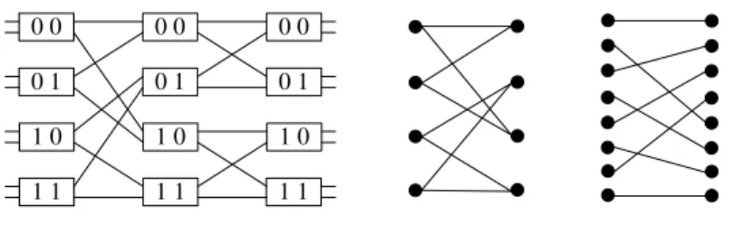
is a network with s columns (stages) where each column consists of N/d d × d crossbars (switches) such that links exist only between crossbars of adjacent stages (note that we do not allow multi-links between crossbars). An n-stage network is a banyan network if each input has a unique path to each output (see Figure 1). If a network has more than
∗This research was partially supported by the National Science Council of the Republic of China under
the grants NSC93-2115-M-009-011 and NSC93-2115-M-009-013.
†The corresponding author, e-mail: [email protected]
‡This paper was written when the author was visiting Center of Mathematical Sciences, Zhejiang
n stages, then we say such a network has extra stages. In all the figures, the arcs are directed from left to right.
0 0 0 1 1 1 1 0 0 0 0 1 1 1 1 0 0 0 0 1 1 1 1 0
Figure 1: A binary 3-stage banyan network (the Baseline network), G1, and G1.
We can associate an s-stage network with a directed graph G in which vertices
rep-resent crossbars and arcs the communication links. Throughout this paper, Gi,j denotes
the subgraph of G induced by the vertices from stage i to stage j. When there is no
confusion, Gi,j also denotes the subnetwork from stage i to stage j. Set Gi = Gi,i+1 for
easy writing (see Figure 1).
Two s-stage networks are topologically equivalent (or simply equivalent) if their associ-ated directed graphs are isomorphic. In other words, two s-stage networks are equivalent if one can be obtained from the other by permuting crossbars in the same stage. Note that equivalence in this sense preserves the connecting properties of the network. Hence once we prove a nonblocking property for a network, it extends to all equivalent networks. Parker [10] first established the equivalence of several n-stage banyan networks includ-ing the Baseline network. Wu and Feng [13] expanded the equivalence class. Dais and
Jump [6] introduced the “buddy” notation: Let v and v0be two crossbars in stage i and let
Vv and Vv0 be two sets of crossbars in stage j that v and v0 can reach, respectively. Then
the network is a buddy network if for any i and j = i + 1, either Vv = Vv0 or Vv∩ Vv0 = ∅.
Agrawal [1] called a buddy network a strict buddy network if the buddy condition also holds for j = i + 2. In this paper, we further generalize the strict buddy network to the universal buddy network by allowing j to be arbitrary. In [1], Agrawal claimed that the strict buddy property characterizes the Baseline-equivalent networks. Bermond, Fourneau and Jean-Marie [2, 3] gave a counterexample to Agrawal’s claim. Instead, they defined
the P (∗, ∗) property for characterization: A network is a P(∗, ∗) network if for any two
stages i ≤ j, the number of components in the subgraph Gi,j is dn−1−(j−i).
Siegel and Smith [12] proposed an extra stage to the Baseline-equivalent class of net-works, and Shyy-Lea [11] considered the k-extra-stage version. Hwang, Liao and Yeh (see [8]) pointed out that the extra stage versions of Baseline-equivalent networks are not necessarily equivalent. Equivalence depends not only on the base network (Baseline or others), but also on how the extra stages are added. Previously, equivalence of extra-stage networks has been studied only for the double-concatenation type [4, 7] since it contains the famous Beneˇs network as a special case.
To study the equivalence of extra-stage networks for arbitrary number of stages, Chang, Hwang and Tong [5] proposed the class of bit permutation networks. Label
the crossbars in a stage by distinct d-nary (n − 1)-sequences x1x2· · · xn−1. A bit-i group
(or simply an i-group) consists of the d crossbars whose labels differ only in bit i (there
are dn−2 bit-i groups). An s-stage network is a bit permutation network if for every G
i,
1 ≤ i ≤ s − 1, the links always go from bit-ui groups G0 of stage i to bit-vi+1 groups G00
of stage i + 1 for some ui, vi+1, where G00 is a permutation of G0. (A detailed definition of
bit permutation networks is in Section 2.) They proved that a bit permutation network
is equivalent to one whose Gi has the property that vi+1 = ui for all i. Such a network
can be characterized by the vector (u1, u2, · · · , us−1).
Recently, Li [9] proposed the bit permuting network. He view the outputs of stage i
and the inputs of stage i+1 as the vertices of a bipartite graph Gi and label the outputs of
stage i (inputs of stage i+1) by distinct d-nary n-sequences; see Figure 1. Then Gi gives a
bijection from the dn outputs to the dn inputs and hence can be treated as a permutation.
Such a permutation is called an bit permutation if it can be characterized by a permutation
σi of the n bits. A network is a bit permuting network if each Gi corresponds to a σi. Li
gave an elegant “guide” algorithm to route any n-stage bit permuting network.
The notions of universal buddy (UB), bit permutation (BP ) and bit permuting (BP T ) are applicable to networks with any number of stages. Since P (∗, ∗) is defined only for
n-stage networks, we generalize it to the power-of-d networks. An s-stage network is a
power-of-d network if for any i, j, 1 ≤ i ≤ j ≤ s, the number of components in Gi,j is
a power of d. An s-stage network is a power-of-d universal buddy network if it is both
power-of-d and universal buddy. The notion of power-of-d (dP) and power-of-d universal
buddy (dPUB) are applicable to networks with any number of stages. In this paper, the
notations of UB, BP , BP T , dP and dPUB also denote their corresponding classes of
networks.
Let A ⊃ B denote A properly contains B. Let A = B denote A is equal to B, meaning any network in class A is a network in class B (no permutation of crossbars allowed), and vice versa. Let A ∼ B denote A is equivalent to B, meaning any network in class A is topologically equivalent to a network in class B (permutations of crossbars allowed), and vice versa. Note that the permutation of crossbars is neither unique nor one-to-one. Hence A ∼ B does not imply |A| = |B|. In particular, A ⊃ B does not preclude A ∼ B. In this paper, we will establish:
UB ⊃
dP ⊃ dPUB ⊃ BP = BP T. (1.1)
dPUB ∼ BP, but UB dP, UB dPUB and dP dPUB. (1.2)
Since the BP network has the vector characterization and is defined for any number of stages, it is of interests to know whether this very useful class can be further extended
with all connecting properties preserved. (1.1) shows that dPUB generalizes BP and (1.2)
shows that they are equivalent.
2
The BP and BP T classes
We now give a detailed definition of BP networks; this definition is from [5]. An
s-stage network is a bit permutation network if for every Gi, 1 ≤ i ≤ s − 1, there exists
a permutation ρi on {1, 2, · · · , n} such that ρi(n) 6= n and each crossbar x1x2· · · xn−1 is
adjacent to crossbar xρi(1)xρi(2)· · · xρi(n−1), where xn ∈ {0, 1, · · · , d − 1}. Note that xn
by running xn through the set {0, 1, · · · , d − 1}. For example, the network in Figure 1 is
a bit permutation network with ρ1 = (132) and ρ2 = (23). Since ρ1 = (132), x1x2x3 is
mapped to x3x1x2 and the links go from bit-2 groups of stage 1 to bit-1 groups of stage
2. In particular, crossbars 00 and 01 at stage 1 are adjacent to crossbars 00 and 10 at
stage 2. Since ρ2 = (23), x1x2x3 is mapped to x1x3x2 and the links go from bit-2 groups
of stage 2 to bit-2 groups of stage 3. Thus crossbars 00 and 01 at stage 2 are adjacent to crossbars 00 and 01 at stage 3.
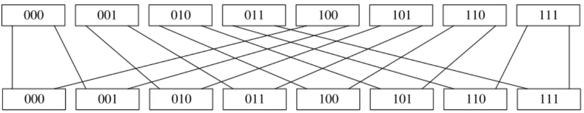
The stages in Figure 2 and Figure 3 are drawn horizontally to save space. These two figures are the same (they have the same connections between crossbars) except their labels. The labels in Figure 2 are outputs of stage i and inputs of stage i + 1. The labels in Figure 3 are crossbars of stage i and crossbars of stage i + 1. The permutation in
Figure 2 illustrates a bit permutation σi = (1234) in Gi, while the permutation in Figure
3 illustrates a permutation ρi = (1234) in Gi.
0010 0011
0000 0001 0100 0101 0110 0111 1000 1001 1010 1011 1100 1101 1110 1111
0010 0011
0000 0001 0100 0101 0110 0111 1000 1001 1010 1011 1100 1101 1110 1111
Figure 2: A bit permutation σi in Gi.
001
000 010 011 100 101 110 111
001
000 010 011 100 101 110 111
Figure 3: A permutation ρi of crossbars in Gi.
We now prove
Proof. First consider a BP T network. For every Gi, there exists a bit permutation
σi on {1, 2, · · · , n} such that each output x1x2· · · xn of stage i is adjacent to input
xσi(1)xσi(2)· · · xσi(n)of stage i + 1. Note that the label of a crossbar of stage i (i + 1) can be
obtained from the labels of its d outputs (inputs) by dropping the last bit. Thus crossbar
x1x2· · · xn−1is adjacent to crossbar xσi(1)xσi(2)· · · xσi(n−1). Note that σi(n) 6= n; otherwise,
there are multi-links between crossbar x1x2· · · xn−1 and crossbar xσi(1)xσi(2)· · · xσi(n−1).
Since σi(n) 6= n, crossbar x1x2· · · xn−1is adjacent to crossbar xσi(1)xσi(2)· · · xσi(n−1), where
xn ∈ {0, 1, · · · , d − 1}. Thus a BP T network is a BP network. On the other hand,
consider a BP network. For every Gi, there exists a permutation ρi on {1, 2, · · · , n}
such that ρi(n) 6= n and each crossbar x1x2· · · xn−1 of stage i is adjacent to crossbar
xρi(1)xρi(2)· · · xρi(n−1) of stage i + 1, where xn ∈ {0, 1, · · · , d − 1}. Thus each output
x1x2· · · xnof stage i is adjacent to input xρi(1)xρi(2)· · · xρi(n) of stage i + 1. Since a
permu-tation on {1, 2, · · · , n} is a bit permupermu-tation, a BP network is a BP T network. Theorem 1 now follows.
We now show that a bit permutation σi of Gi defines a mapping from u-groups of stage
i to v-groups of stage i + 1. In fact, we can pinpoint u and v.
Lemma 2 Suppose Gi is represented by the bit permutation σi. Then Gi induces a
map-ping from σi(n)-groups of stage i to σi−1(n)-groups of stage i + 1.
Proof. Note that each output x1x2· · · xnof stage i is adjacent to input xσi(1)xσi(2)· · · xσi(n)
of stage i + 1. The label of a crossbar of stage i (i + 1) can be obtained from the labels
of its d outputs (inputs) by dropping the last bit. Since xσi(n) is the last bit and get
dropped in the crossbar label of stage i + 1, the d stage-i crossbars differing only in bit
σi(n), i.e., the σi(n)-group, are mapped to the same set of stage-(i + 1) crossbars. On the
other hand, the stage-i crossbar containing d outputs whose labels differ only in bit σi(n)
is mapped to the σ−1
i (n)-group of stage i + 1. Lemma 2 is proved.
(σ−1i (4) = 3)-groups of stage i + 1. We now give a vector characterization of a BP T network. First a lemma.
Lemma 3 Suppose Gi corresponds to a bit permutation σi which maps σi(n)-groups of
stage i to σi−1(n)-groups of stage i + 1 and suppose Gi+1 corresponds to a bit permutation
σi+1. Suppose we permute the crossbars of stage i + 1 such that the j-th crossbars of the
σ−1
i (n)-groups are lined up with the j-th crossbars of the σi(n)-groups, j = 0, 1, · · · , d − 1.
Then after the lining-up operation, Gi corresponds to the bit permutation (ui n) and Gi+1
corresponds to the bit permutation (σ−1
i+1(σi−1(n)) σ−1i+1(σi(n))) ◦ σi+1.
Proof. Take a σ−1
i (n)-group of stage i+1. The j-th crossbar in this group is mapped (lined
up) to the j-th crossbar of the corresponding σi(n)-group of stage i under this lining-up
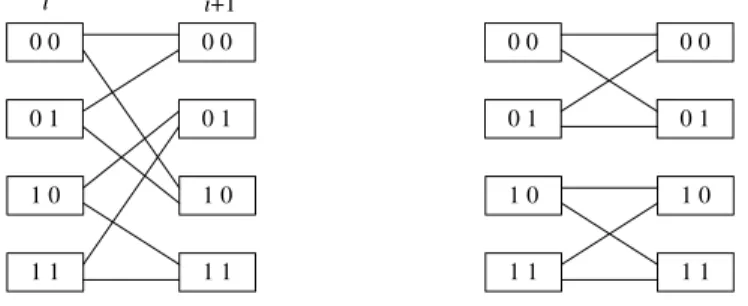
operation; see Figure 4. Then the only difference is that before lining up, the bit
permu-tation σi maps σi(n)-groups to σi−1(n)-groups, while after lining up, the mapping is from
ui-groups to ui-groups. Note that the mapping from ui-groups to ui-groups corresponds
to the bit permutation (ui n). After lining up, σi−1(n)-groups of stage i + 1 become σi
(n)-groups. Since σi+1 maps σi+1−1(σ−1i (n)) to σi−1(n) and σ−1i+1(σi(n)) to σi(n), swapping bit
σ−1
i (n) with bit σi(n) corresponds to applying (σi+1−1(σi−1(n)) σ−1i+1(σi(n))) on σi+1. Thus
after lining up, Gi+1 corresponds to bit permutation (σi+1−1(σ−1i (n)) σ−1i+1(σi(n))) ◦ σi+1.
0 0 0 1 1 1 1 0 i i+1 0 0 0 1 1 1 1 0 0 0 0 1 1 1 1 0 0 0 0 1 1 1 1 0
Figure 4: Lining up stage-(i + 1) crossbars.
By Lemma 2, we know that in every Gi of a BP T network, the links go from ui
-groups to vi+1-groups for some ui, vi+1. The lining-up operation enables us to permute
in Figure 4, the links go from 2-groups to 1-groups. After lining up the stage-(i + 1) crossbars, the links go from 2-groups to 2-groups.
Theorem 4 Consider an s-stage BP T network. By permuting the crossbars of stage 2,
3, · · · , s, each Gi corresponds to a bit permutation which maps u0i-groups to u0i-groups,
i = 1, 2, · · · , s − 1.
Proof. We prove this theorem by induction on s. This theorem is trivially true for s = 2 since we can permute the crossbars of stage 2 to line up with their mates in stage 1. Then
G1 corresponds to a bit permutation which maps u1-groups to u1-groups. Suppose this
theorem holds for up to s − 1 stages. We now prove for s stages. Again, permute the
crossbars of stage 2 to line up with their mates in stage 1. By Lemma 3, G2 remains
to correspond to a bit permutation. Thus we may apply induction on this (s -1)-stage
BP T network such that Gi is characterized by a bit permutation which maps u0i-groups
to u0
i-groups, i = 1, 2, · · · , s − 1.
Since BP T = BP , the above characterization is also a vector characterization of a BP network, but our proof is simpler than the original proof in [5]. Recall that an s-stage
network is a BP network if for every Gi, the links always go from ui groups G0 of stage i
to vi+1 groups G00 of stage i + 1 for some ui, vi+1, where G00 is a permutation of G0. If we
drop the requirement that G00 is a permutation of G0, then the lining-up operation would
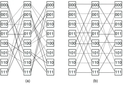
not yield a vector characterization. See Figure 5 as an example. In Figure 5(a), the links
in G1 go from 1-groups to 2-groups and the links in G2 go from 1-groups to 3-groups. In
Figure 5(b), the links in G1 go from 1-groups to 1-groups, but the links in G2 do not go
from u-groups to u-groups for any u.
3
The d
PUB class
We now show that neither dP ⊆ UB nor vice versa; hence the definition of dPUB makes
000 001 010 011 100 101 110 111 000 001 010 011 100 101 110 111 000 001 010 011 100 101 110 111 000 001 010 011 100 101 110 111 000 001 010 011 100 101 110 111 000 001 010 011 100 101 110 111 (a) (b)
Figure 5: (a) Before lining up and (b) after lining up.
D0, F0, G0} and E reaches {C0, E0, F0, H0}; the two sets intersect but are not identical.
Figure 6(b) shows a UB network which is not a 2P network since G
1,3 has 3 components. C D E F G H C D E F G H
Figure 6: (a) A 2P network and (b) a UB network.
We first quote a result of [5].
Theorem 5 Suppose an s-stage d-nary BP network has dn inputs, dn outputs, and is
characterized by the vector (u1, u2, · · · , us−1) which contains k distinct elements. Then the
Corollary 6 BP ⊆ dP.
Proof. It is not difficult to see that every subnetwork Gi,j of a BP network is still a BP
network. By Theorem 5, the number of components in Gi,j is a power of d. Since i, j are
arbitrary, the network is in dP.
Theorem 7 BP ⊆ UB.
Proof. Consider an s-stage BP network characterized by (u1, u2, · · · , us−1). Let v be
a crossbar in stage i which reaches a set Vj(v) of crossbars in stage j. Then Vj(v)
con-sists of crossbars whose labels are the same in bits in the set I = {1, 2, · · · , n − 1} \
{ui, ui+1, · · · , uj−1}. Let v0 be another crossbar in stage i. If v0 differs from v in a bit in I,
then clearly, Vj(v0) ∩ Vj(v) = ∅; if not, then Vj(v0) = Vj(v). Since i, j, v, v0 are arbitrary,
the network is in UB.
Theorem 8 BP ⊂ dPUB.
Proof. That BP ⊆ dPUB follows from Corollary 6 and Theorem 7. That the
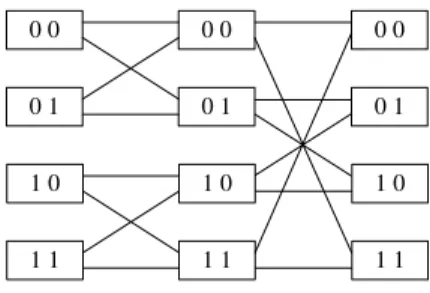
con-tainment is strict follows from Figure 7 (crossbars 00 and 11 in stage 2 are connected to crossbars 00 and 11 in stage 3; so, the links from stage 2 to stage 3 do not go from
ui-groups to vi+1-groups for any ui, vi+1).
0 0 0 1 1 1 1 0 0 0 0 1 1 1 1 0 0 0 0 1 1 1 1 0
Figure 7: A dPUB network which is not a BP network.
Proof. Since dPUB ⊃ BP T , it suffices to prove that a dPUB network is equivalent to a BP network. We prove this by induction on the number s of stages.
(1) s = 2. Suppose v of stage 1 is connected to the set V2(v). Let v0 be another crossbar
in stage 1 and connected to a given w ∈ V2(v). By the UB property, V2(v0) = V2(v).
Since there are d − 1 choices of v0 from w, these v0 together with v form a d × d
complete bipartite graph Kd,d with V2(v). Further, V2(v00) ∩ V2(v) = ∅ for any
v00 6∈ v ∪ {v0}. Since v is arbitrary, G
1,2 consists of dn−2 Kd,d whose equivalence to
a BP network is clear.
(2) s = 3. By the dP property, the network has dn−k components for some 1 ≤ k ≤ n.
Recall that from (1) the subgraphs G1,2 and G2,3 must each consist of dn−2 Kd,d.
Hence k = 1 is impossible.
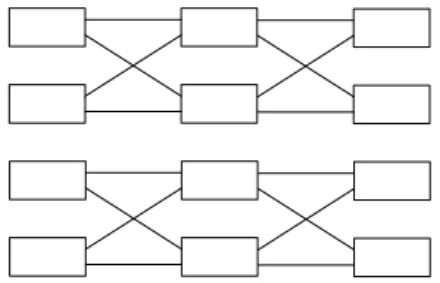
For k = 2, then no two Kd,d in G1,2 can be connected through G2,3. Therefore G1,3
must consist of dn−2 copies of concatenation of two K
d,d, with the outputs of the
former identified with the inputs of the latter (see Figure 8). Clearly, subnetwork
G1,3 is equivalent to a BP network.
Figure 8: Concatenation of K2,2.
For k = 3, first suppose G1,3 is obtained by connecting each d-set D = {D1, D2,
· · ·, Dd}, where each Di is a Kd,d in G1,2, into one component in G1,3. Note that
the connection is done by a d-set D0 = {D0
1, D20, · · · , D0d} of Kd,d in G2,3. If two
be connected to D0
j, violating the UB property. Therefore, the d crossbars in a Di
must go to distinct D0
j, or all D0j. Since we can permute the stage-2 crossbars in a
D arbitrarily, and independently for each D, the stage-2 crossbars in each D can be
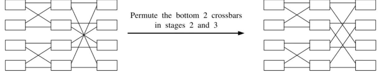
ordered such that the k-th one goes to the k-th D0, which is clearly a BP network.
Figure 9 illustrates how to permute.
Permute the bottom 2 crossbars in stages 2 and 3
Figure 9: A permutation to achieve BP .
Suppose G1,3 is obtained otherwise. There must exist a d0-set of Kd,d, d0 > d, in
G1,2 connected in G2,3 through a d0-set of Kd,d in G2,3. Note that an input in this
component touches only d2 among the dd0 outputs. Hence there must exist another
input reaching some, but not all, of these d2 outputs, violating the UB property.
For k ≥ 4, then the situation described in the last paragraph must also happen.
(3) s ≥ 4. Consider the two subnetworks G1,3 and G2,s. By induction, G1,3 can be
represented by a vector (u1, u2) and G2,s by (u01, u02, · · · , u0s−2). By Lemma 3, we can
permute the crossbars in stage k, 2 ≤ k ≤ s, such that u0
1 = u2 and u00k = u0k−1
for 3 ≤ k ≤ s − 1. Therefore the subnetwork G1,s is represented by the vector
(u1, u2, u003, · · · , u00s−1), i.e., G1,s is a BP network.
Corollary 10 Two dPUB networks are equivalent if the characterization vector of one
Figure 6(a) gives an example of a dP network which is not equivalent to a UB network.
Hence dP UB. Since UB ⊃ BP , Figure 6(a) is also an example of a dP network which
is not equivalent to a BP network. Therefore the UB condition can not be dropped from
Theorem 9. Since BP ∼ dPUB, it follows that dP dPUB. Figure 6(b) gives a UB
(or strict buddy) network which is equivalent to neither a dP nor a BP network. Hence
UB BP . Since BP ∼ dPUB, it follows that UB dPUB.
4
Conclusions
We established the containment relation as given in (1.1), and the equivalence relation as given in (1.2). By so doing, we achieve three desirable generalizations:
(1) We make the logical extension of the buddy network and the strict buddy network to the universal buddy network; a network with more structure but still includes all banyan-type networks and their extra-stage versions.
(2) We generalize the notion of BP to dPUB which is a larger class, yet preserves all
connecting properties of BP .
(3) We generalize P (∗, ∗) which is defined only for n = logdN stages to general s stages.
The equivalence relations we established also help in simplifying some existing proofs: (1) The proof of vector characterization of BP in [5] is quite complicated. We gave a simple proof of vector characterization of BP T and the equality that BP T = BP makes the proof valid for BP too.
(2) The proof that P (∗, ∗) characterizes the Baseline-equivalent class of banyan-type networks is very long, as admitted in [2]. Our proofs of Theorem 9 and Corollary 10 are much shorter and more general.
Acknowledgement.
The author wishes to thank H. Zhou for providing acounterex-ample to a conjecture prior to our discovery of Theorem 9. We also thank the comments of referees which led to a better version of the paper.
References
[1] D.P. Agrawal, Graph theoretical analysis and design of multistage interconnection networks, IEEE Trans. Comput. 32 (1983) 637-648.
[2] J.C. Bermond, J.M. Fourneau and A. Jean-Marie, Equialence of multistage intercon-nection networks, Inform. Proc. Lett. 26 (1987) 45-50.
[3] J.C. Bermond, J.M. Fourneau and A. Jean-Marie, A graph theoretical approach to equivalence of multistage interconnection networks, Disc. Appl. Math. 22 (1988/89) 201-217.
[4] T. Calamoneri and A. Massini, Efficient algorithm for checking the equivalence of multistage interconnection networks, J. Parallel Distrib. Comput. 64 (2004) 135-150. [5] G.J. Chang, F.K. Hwang and L.D. Tong, Characterizing bit permutation networks,
Networks 33 (1999) 261-267.
[6] D.M. Dias and J.R. Jump, Analysis and simulation of buffered delta networks, IEEE Trans. Comput. C-30 (1981) 273-282.
[7] Q. Hu, X. Shen and J. Yang, Topologies of combined (2 log N − 1)-stage intercon-nection networks, IEEE Trans. Comput. 46 (1997) 118-124.
[8] F.K. Hwang, The Mathematical Theory of Nonblocking Switching Networks, World Scientific, Singapore, 1998.
[9] S.-Y.R. Li, Algebraic Switching Theory and Broadband Applications, Academic, New York, 2001.
[10] D.S. Parker, Notes on shuffle-exchange type of networks, IEEE Trans. Comput. 29 (1980) 213-222.
[11] D.J. Shyy and C.T. Lea, Log2(N, m, p) strictly nonblocking networks, IEEE Trans.
[12] H.J. Siegel and S.D. Smith, Study of multistage SIMD interconnection networks, Proc. 5-th Ann. Symp. Comput. Arch., 1978, 223-229.
[13] C. Wu and T. Feng, On a class of multistage interconnection networks, IEEE Trans. Comput. 29 (1980) 694-702.
On Degenerate Double-Loop L-Shapes
∗
J. S. Lee
Department of Mathematics, National Kaohshiung Normal University Kaoshiung 802, Taiwan
James K. Lan and Jenny C. Chen
†Department of Applied Mathematics, National Chiao Tung University Hsinchu 300, Taiwan
Abstract
Most of the results about the L-shapes of double-loop networks are given in terms of the four parameters `, h, p, n. But these parameters are not well defined in the degenerate case. Recently, Cheng and Hwang gave an efficient algorithm to compute the four parameters `, h, p, n of an L-shape which works for both the regular and the degenerate cases. On the other hand, Chen and Hwang gave a set of rules to determine the four parameters of a degenerate L-shape. Unfortunately, the solutions given by the above two methods do not always coincide. In this paper, we try to understand their respective meanings and their relations.
Keywords: Double-loop network, L-shape, degenerate.
1
Introduction
The double-loop network has been well studied (see [6] for a recent survey) as the topology for a communication network or computer network. For example, SONET (synchronous optical network) is a double-loop network. Formally, a double-loop network DL(N; a, b) has N nodes 0, 1, · · · , N −1 and 2N links, i → i+a, i → i+b (mod N), i = 0, 1, · · · , N −
∗This research was partially supported by the National Science Council of the Republic of China under
the grant NSC93-2115-M-009-011.
†e-mail: [email protected]
1. We assume that the weight of each of the 2N links is 1 and assume that gcd(N, a, b) = 1 so that the network is strongly connected.
The minimum distance diagram (MDD) of DL(N; a, b) is a diagram with node 0 in cell (0, 0), and node v in cell (i, j) if and only if ia + jb ≡ v (mod N) and i + j is the
minimum among all (i0, j0) satisfying the congruence. Namely, a shortest path from 0 to
v is through taking i a-links and j b-links (in any order). Note that in a cell (i, j), i is the column index and j is the row index. An MDD includes every node exactly once (in case of two shortest paths, the convention is to choose the cell with the smaller row index, i.e., the smaller j). Since DL(N; a, b) is clearly node-symmetric, there is no loss of generality in assuming: node 0 is the origin of a path.
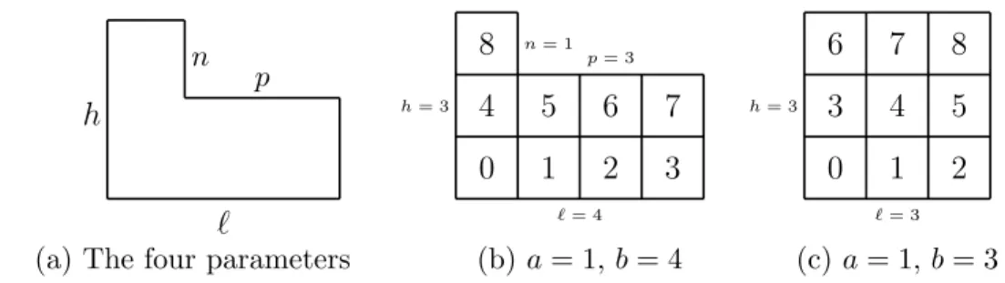
Wong and Coppersmith (WC) [8] proved that the MDD of DL(N; a, b) (their proof for DL(N; 1, h) is easily extended to the general case) is always an L-shape which can be characterized by four parameters `, h, p, n (see Fig. 1 (a)). These four parameters are the lengths of four of the six segments on the boundary of the L-shape. Clearly,
N = `h − pn.
In [2], Chen and Hwang showed that necessarily ` > n and h ≥ p. Fig. 1 (b) illustrates an MDD with a regular L-shape. Fig. 1 (c) illustrates one with an L-shape degenerate into a rectangle.
h
`
p n
(a) The four parameters
0 1 2 3 4 5 6 7 8 ` = 4 h = 3 n = 1 p = 3 (b) a = 1, b = 4 0 1 2 3 4 5 6 7 8 ` = 3 h = 3 (c) a = 1, b = 3
Figure 1: Minimum distance diagrams and L-shapes.
Most of the results about the L-shape are given in terms of the four parameters `, h, p, n. But these parameters are not well defined in the degenerate case. Recently,
Cheng and Hwang [4] gave an O(log N)-time algorithm to compute the four parameters `, h, p, n of an L-shape which works for both the regular and the degenerate cases. On the other hand, Chen and Hwang [3] gave a set of rules to determine the four parameters of a degenerate L-shape. Unfortunately, the solutions given by the above two methods do not always coincide. In this paper, we try to understand their respective meanings and their relations. Since it is also of interest to know when will an L-shape degenerate, in this paper we give necessary and sufficient conditions depending on N, a, and b only.
2
Necessary and sufficient conditions for degenerate
L-shapes
The following five notations will be used throughout this paper:
d = gcd(N, a), d0 = gcd(N, b), N0 = N/d, a0 = a/d, and b0 = b (mod N0). (2.1)
Since gcd(N, a, b) = 1, clearly gcd(d, d0) = 1. Chen and Hwang [3] proved
Lemma 1 [3] A degenerate L-shape of height h and width ` satisfies one of the following three conditions:
(1) hb 6≡ `a ≡ 0 (mod N). (2) `a 6≡ hb ≡ 0 (mod N). (3) `a ≡ hb ≡ 0 (mod N).
We now prove
Theorem 2 The L-shape of DL(N; a, b) is degenerate if and only if one of the following three conditions holds:
(C1) d > 1 and there exists 1 ≤ i ≤ min{d,N
d − 1} such that db ≡ ia (mod N).
(C2) d0 > 1 and there exists 1 ≤ j ≤ min{d0− 1,N
d0 − 1} such that d0a ≡ jb (mod N).
(C3) d > 1, d0 > 1 and d0a ≡ db ≡ 0 (mod N).
Moreover, (C1) ⇔ (1), (C2) ⇔ (2) and (C3) ⇔ (3). Also, if (C1) holds, then the degenerate shape is of height d and width N/d; if (C2) holds, then the degenerate
L-shape is of height N/d0 and width d0; if (C3) holds, then the degenerate L-shape is of height
d and width d0.
Proof. Necessity. Suppose the L-shape is degenerate and is a rectangle of height h and
width `. Then by Lemma 1, it satisfies (1) or (2) or (3). We first prove two claims. Claim 1. If `a ≡ 0 (mod N), then h = d, ` = N/d and d > 1.
Proof of Claim 1. Let a = αd for some integer α. Note that the L-shape being degenerate implies N = `h. Thus `a ≡ 0 (mod N) implies a ≡ 0 (mod h). Let a = βh
for some integer β. Then a = αd = βh. Hence d = βhα. Since 1 = gcd(α,N
d) = gcd(α, `h βh α ) = gcd(α,`α β), necessarily α|β. Therefore β
α is an integer. Since d|N, we have
β α|`. Suppose β α > 1. Let `0 = `β α . Then `0 < ` and `0a = ` β α βh = `hα = Nα ≡ 0 (mod N). Then row 0 of the L-shape will contain two entries of 0, one at cell (0,0) and the other at
cell (`0, 0), a contradiction to the definition of an L-shape (recall that an MDD includes
every node exactly once). Therefore β
α = 1. Consequently, h = d and ` = N/d. Since
` < N and `d = N, clearly d > 1.
Claim 2. If the L-shape is degenerate and hb ≡ 0 (mod N), then h = N/d0, ` = d0
and d0 > 1.
Proof of Claim 2. Since this proof is similar to that of Claim 1, we omit it.
We now prove the necessity of this theorem. First, assume the L-shape satisfies condition (1). By Claim 1, we have d > 1, h = d and ` = N/d. By the definition of an MDD, hb is the first element in column 0 satisfying
hb ≡ ia + jb (mod N) with i + j ≤ h, i ≥ 0, j ≥ 0.
Therefore j = 0 for otherwise (h−j)b would be the first element. Also, i ≥ 1 for otherwise hb ≡ 0 (mod N). Thus db = hb ≡ ia (mod N) for 1 ≤ i ≤ d. Since ` = N/d, we have
i ≤ N
d − 1. We conclude db ≡ ia (mod N) for 1 ≤ i ≤ min{d,Nd − 1}, which means (C1)
holds. The above discussion also shows that (1) implies (C1), i.e., (1) ⇒ (C1).
Next, assume the L-shape satisfies condition (2). Then the argument is similar except at the end we have
`a ≡ ia + jb (mod N) with i + j < `, i ≥ 0, j ≥ 0.
The reason for the strict inequality that i + j < ` is by our construction on tie-breaking in defining the MDD. Thus (C2) holds. So (2) ⇒ (C2).
Finally, assume the L-shape satisfies condition (3). By Claim 1, we have d > 1, h = d
and ` = N/d. By Claim 2, we have d0 > 1, h = N/d0 and ` = d0. Thus d0a = `a ≡ 0
(mod N) and db = hb ≡ 0 (mod N), which means (C3) holds. So (3) ⇒ (C3).
Sufficiency. Let the L-shape of DL(N; a, b) be (`, h, p, n). First, assume that (C1) is
satisfied. Since db ≡ ia (mod N) for 1 ≤ i ≤ min{d,N
d − 1}, we have h ≤ d. On the
other hand, ` ≤ N/d since (N/d)a = N(a/d) ≡ 0 (mod N). Therefore N = `h − pn ≤ `h ≤ (N/d)d = N.
Necessarily,
` = N/d, h = d. It follows
`h = N,
i.e., the L-shape is degenerate. Moreover, `a = (N/d)a = N(a/d) ≡ 0 (mod N); hb = db ≡ ia 6≡ 0 (mod N) since 1 ≤ i ≤ ` − 1. So (C1) ⇒ (1).
The proof of (C2) is similar to that of (C1). Finally, assume that (C3) is satisfied.
Then since d0a ≡ db ≡ 0 (mod N), we have ` ≤ d0 and h ≤ d. Since d|N, d0|N and
gcd(d, d0) = 1, we have d0d ≤ N. Therefore
N = `h − pn ≤ `h ≤ d0d ≤ N.
Necessarily,
` = d0, h = d.
It follows
`h = N,
i.e., the L-shape is degenerate. Moreover, `a = d0a ≡ 0 (mod N); hb = db ≡ 0
(mod N). So (C3) ⇒ (3).
Remarks. From the proof of Theorem 2, when an L-shape(`, h, p, n) degenerates into a rectangle, it is reasonable to set ` to the width and h to the height of the rectangle. Moreover, it is reasonable to set p = 0 or n = 0 since N = `h − pn and `h = N hold simultaneously.
3
Strongly isomorphic double-loop networks and
de-generate L-shapes
The following property was proved in [1].
Lemma 3 [1] If α and β are integers, not both zero, then there exist integers x and y such that yα + xβ = gcd(α, β) and gcd(x, gcd(α, β)) = 1.
Let DL(N; a, b) be a double-loop network. Then
Lemma 4 There exists an integer x such that gcd(x, N ) = 1 and ax ≡ d (mod N).
Proof. Since gcd(N, a) = d, by Lemma 3, there exist integers x and y such that yN +
xa = d and gcd(x, d) = 1. Hence ax ≡ d (mod N). Moreover, y(N/d) + x(a/d) = 1 implies gcd(x, N/d) = 1. It follows that gcd(x, N ) = gcd(x, (N/d)d) = 1. Hence the lemma.
Two double-loop networks DL(N; a, b) and DL(N; a0, b0) are strongly isomorphic if
there exists a z prime to N such that a0 ≡ az, b0 ≡ bz (mod N) or a0 ≡ bz, b0 ≡ az
(mod N) [7]. It is well known that two strongly isomorphic double-loop networks realize the same L-shape. The following property greatly simplifies the proofs in the remaining sections.
Theorem 5 Let x be an integer such that gcd(x, N ) = 1 and ax ≡ d (mod N). Let
b00 = bx (mod N). Then DL(N; a, b) and DL(N; d, b00) are strongly isomorphic.
Proof. This theorem follows from Lemma 4.
In the following, we characterize a degenerate L-shape by the four independent pa-rameters `, h, p, n. Set
m = ` − p, q = h − n for convenience; see Fig. 2(a). Then
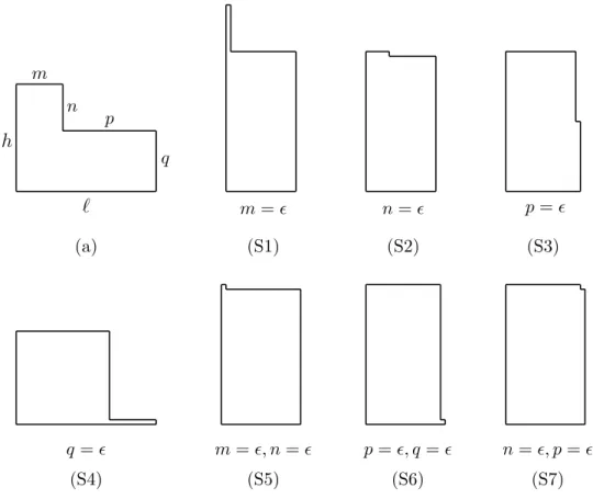
Lemma 6 For a degenerate L-shape, at least one of m, n, p, q is zero and at most two of m, n, p, q are zero. Moreover, it is impossible that both m and p, both n and q, or both m and q are zero.
Proof. It is obvious that at least one of m, n, p, q is zero. Since ` = m+p and h = n+q,
if more than two of m, n, p, q are zero, then ` = 0 or h = 0 will happen, which is impossible. Suppose two of m, n, p, q are zero. If both m and p (n and q) are zero, then ` = m + p = 0 (h = n + q = 0), which is impossible. If both m and q are zero, then ` = p, h = n, and then N = `h − pn = 0, which is also impossible. Hence the lemma.
Corollary 7 There are only seven possible ways to view a degenerate L-shape. We define these shapes by identifying the parameters which are set to zero: (S1): only m = 0, (S2): only n = 0, (S3): only p = 0, (S4): only q = 0, (S5): m = 0 and n = 0, (S6): p = 0 and q = 0, (S7): n = 0 and p = 0.
h ` p n m q (a) m = ² (S1) n = ² (S2) p = ² (S3) q = ² (S4) m = ², n = ² (S5) p = ², q = ² (S6) n = ², p = ² (S7)
Figure 2: The ways to degenerate an L-shape.
By Corollary 7, there are seven ways to view a degenerate L-shape as the product of a limiting process operated on a regular L-shape. Fig. 2 (S2), (S3), (S5), (S6) and (S7) show five processes of shrinking a subrectangle with a side (or two sides) of length approaching zero; Fig. 2 (S1) and (S4) show two processes of cutting off a subrectangle with a side of length approaching ` or h. When ² = 0, they all represent the same rectangle. But the different underlying process can induce different values of (`, h, p, n).
Fiol, Yebra, Alegre, and Valero [5] pointed out that an L-shape, regular or degenerate, always tessellates the plane. Then (`, −n) and (−p, h) are simply two independent vectors characterizing the distribution of the nodes labelled by 0 (will be referred to as the 0-nodes) as seen by the equations:
`a − nb ≡ 0 (mod N)
−pa + hb ≡ 0 (mod N). (3.2)
Note that (`, −n) is a vector in the fourth quadrant, and (−p, h) one in the second. But there are other choices of two independent vectors.
4
Cheng-Hwang’s algorithm
Cheng and Hwang [4] gave an algorithm (CH-ALGO in short) to solve for (`, h, p, n) for DL(N; a, b). The algorithm works regardless whether the L-shape is regular or not. For completeness, we give a brief review of this algorithm (note that the weight of each link in the given double-loop network is assumed to be 1).
CHENG-HWANG-ALGORITHM. Input: DL(N; a, b).
Output: (`, h, p, n) of the L-shape of DL(N; a, b).
Let d, d0, N0, a0 and b0 be defined as in (2.1).
Let s0 be the integer with
a0s
0+ b0 ≡ 0 (mod N0), 0 ≤ s0 < N0.
Let s−1 = N0 and define qi, si, recursively (by the Euclidean algorithm) as follows:
s−1 = q1s0+ s1, 0 ≤ s1 < s0 s0 = q2s1+ s2, 0 ≤ s2 < s1 s1 = q3s2+ s3, 0 ≤ s3 < s2 · · · sk−2 = qksk−1+ sk, 0 ≤ sk< sk−1 sk−1 = qk+1sk, 0 = sk+1 < sk. (4.3)
Define integers Ui by U−1 = 0, U0 = 1, and
Ui+1 = qi+1Ui+ Ui−1, i = 0, 1, · · · , k. (4.4)
By induction,
siUi+1+ si+1Ui = N0, i = 0, 1, · · · , k. (4.5)
Regard s−1/U−1 = ∞ > x for real number x. Since {si}k+1i=−1 and {Ui}k+1i=−1 are strictly
decreasing and increasing, respectively, we have
0 = sk+1 Uk+1 < sk Uk < · · · < s0 U0 < s−1 U−1 = ∞. 9
Let u be the largest odd integer such that d < su Uu. Define v = » su− dUu su+1+ dUu+1 ¼ − 1. Let
`0 = su− vsu+1, h0 = Uu+ (v + 1)Uu+1, p0 = su− (v + 1)su+1, n0 = Uu+ vUu+1.
Then
(`, h, p, n) = (`0, dh0, p0, dn0). End-of-CHENG-HWANG-ALGORITHM.
Now we characterize the (`, h, p, n) obtained by CH-ALGO when DL(N; a, b) has a degenerate L-shape. By Theorem 5, it suffices to consider the case that a|N. Since a|N, CH-ALGO derives
d = a, d0 = gcd(N, b), N0 = N/d = N/a, a0 = 1, b0 = b (mod N0), s−1 = N0.
So we have
Lemma 8 si ≡ (−1)iUis0 (mod N0) for 1 ≤ i ≤ k + 1.
Proof. By (4.3) and (4.4), s1 = s−1− q1s0 = N0− U1s0, s2 = s0− q2s1 = s0− q2(N0−
U1s0) = −q2N0+(1+q2U1)s0 = −q2N0+U2s0. Thus s1 ≡ (−1)1U1s0 (mod N0) and s2 ≡
(−1)2U
2s0 (mod N0). We prove the general case by induction on i. Assume this lemma
holds for i ≤ t. Then, by (4.3) and (4.4), st+1 = st−1− qt+1st and Ut+1 = Ut−1+ qt+1Ut.
Thus by induction, st+1 ≡ (−1)t−1Ut−1s0− qt+1(−1)tUts0 (mod N0) = (−1)t+1(U t−1+ qt+1Ut)s0 (mod N0) = (−1)t+1Ut+1s0 (mod N0). 10
Theorem 9 If DL(N; a, b) satisfies
(C1), then CH-ALGO derives an L-shape of shape (S2) with (`, h, p, n) = (N0, d, i, 0);
(C2), then CH-ALGO derives an L-shape of shape
(S1) with (`, h, p, n) = (d0, j +ld0−j N d0 m N d0, d0, j + ( l d0−j N d0 m − 1)N d0) if j < 2dN0; (S3) with (`, h, p, n) = (d0,N d0, 0, j) if j ≥ 2dN0; (C3), then CH-ALGO derives an L-shape of shape
(S1) with (`, h, p, n) = (d0,§d0 d ¨ d, d0, (§d0 d ¨ − 1)d) if d < d0; (S5) with (`, h, p, n) = (d0, d, d0, 0) if d > d0.
Proof. First suppose DL(N; a, b) satisfies (C1). Then there exists 1 ≤ i ≤ min {d, N0−
1} such that db ≡ ia (mod N). Since a = d, we have b ≡ i (mod N0). Since b0 = b
(mod N0) and 1 ≤ i ≤ N0− 1, it follows that
b0 = i.
By (4.3), we have s−1 = q1s0 + s1 and q1 ≥ 1. Note that s0 = N0− b0 and U1 = q1. So
s1 U1 = s1 q1 = s−1 q1 − s0 = N0( 1 q1 − 1) + b0 ≤ b0 = i ≤ d.
Therefore u = −1. Since b0 = i ≤ d, N0 ≤ (N0 − b0) + d; therefore l N0
(N0−b0)+d m = 1. Thus v = l s−1−dU−1 s0+dU0 m − 1 = l N0 (N0−b0)+d m − 1 = 0. Hence, m = s0 = N0 − b0 > 0, n =
d(U−1+ vU0) = 0, p = s−1− (v + 1)s0 = b0 = i > 0, q = dU0 = d > 0. Thus the L-shape
is of shape (S2) and
(`, h, p, n) = (N0, d, i, 0).
Now suppose DL(N; a, b) satisfies (C2). So DL(N; a, b) does not satisfy (C3). Hence
N > dd0. Assume that N = dd0N00, where N00 > 1. By Theorem 2, there exists 1 ≤ j ≤
min {d0 − 1, N/d0 − 1} such that d0a ≡ jb (mod N). Since d = a, we have d0d ≡ jb
(mod N). Since gcd(N, b) = d0 and N = dd0N00, it follows that d|j. Let j = dj0. Then
d0d ≡ dj0b (mod dN0), which implies d0 ≡ j0b (mod N0). Thus
d0 ≡ j0b0 (mod N0).
Note that gcd(N0, b0) = gcd(N0, b) = gcd(N, b). Thus gcd(N0, b0) = d0. We now have
sk = gcd(s−1, s0) = gcd(N0, N0− b0) = gcd(N0, b0) = d0
and sk+1 = 0. By (4.5), skUk+1+ sk+1Uk = N0. Since sk = d0 and sk+1 = 0, it follows that
d0U
k+1 = d0N00. Thus
Uk+1 = N00.
By Lemma 8, sk ≡ (−1)kUks0 ≡ (−1)kUk(N0− b0) ≡ (−1)k+1Ukb0 (mod N0). Since k is
either odd or even, there are two cases: Case 1. k is odd.
Then sk ≡ Ukb0 (mod N0). Since sk = d0 ≡ j0b0 (mod N0), we have Ukb0 ≡ j0b0
(mod N0). Thus (U
k− j0)b0 ≡ 0 (mod N0). Since Uk< Uk+1, Uk < N00. Since j < N/d0,
j0 < N00. By the facts that gcd(N0, b0) = d0 and j0 < N00 and U
k < N00, it follows from (Uk− j0)b0 ≡ 0 (mod N0) that Uk= j0. Then sk Uk = d 0 j0 > d.
Hence u = k. Since dUk = dj0 = j and dUk+1 = dN00 = Nd0,
v + 1 = » sk− dUk sk+1+ dUk+1 ¼ = & d0 − j N d0 ' . Thus m = sk+1 = 0, n = d(j0+ vN00) = j + vNd0 > 0, p = sk− (v + 1)sk+1 = d0 > 0, q =
dUk+1 = Nd0 > 0. So the L-shape is of shape (S1) and
(`, h, p, n) = (d0, j + & d0− j N d0 ' N d0, d 0, j + ( & d0− j N d0 ' − 1)N d0). 12
Note that since k is odd and {Ui}k+1i=−1 are strictly increasing, Uk−1 ≥ 1. Note also that qk+1≥ 2. Thus by (4.4), j = dj0 = dU k = d (Uk+1− Uk−1) qk+1 < d Uk+1 2 = d N00 2 = N 2d0. Case 2. k is even.
Then sk ≡ −Ukb0 (mod N0). Since sk = d0 ≡ j0b0 (mod N0), we have −Ukb0 ≡ j0b0
(mod N0). Thus (U
k+ j0)b0 ≡ 0 (mod N0). Since Uk< Uk+1, Uk < N00. Since j < N/d0,
j0 < N00. By the facts that gcd(N0, b0) = d0 and j0 < N00 and U
k < N00, it follows from
(Uk+ j0)b0 ≡ 0 (mod N0) that
Uk= N00− j0.
Then by (4.3), (4.4) and the facts that qk+1≥ 2 and d0 > j,
sk−1− dUk−1 = qk+1sk− d(Uk+1− qk+1Uk) = qk+1d0− d(N00− qk+1(N00− j0)) = qk+1(d0+ N d0 − j) − N d0 > 0. Hence u = k − 1. Since dUk= d(N00− j0) = Nd0 − j, v + 1 = » sk−1− dUk−1 sk+ dUk ¼ = & qk+1(d0+Nd0 − j) − Nd0 d0+ N d0 − j ' = & qk+1− N d0 d0+ N d0 − j ' = qk+1.
Thus m = sk= d0 > 0, n = d(Uk−1+ (qk+1− 1)Uk) = d(Uk+1− Uk) = d(N00− (N00− j0)) =
j > 0, p = sk−1− qk+1sk = sk+1 = 0, q = dUk = Nd0 − j > 0. So the L-shape is of shape
(S3) and
(`, h, p, n) = (d0,N d0, 0, j).
Note that since Uk−1 ≥ 0 and qk+1≥ 2,
j = dj0 = d(N00− U k) = N d0 − d (Uk+1− Uk−1) qk+1 ≥ N d0 − d N00 2 ≥ N d0 − N 2d0 = N 2d0.
Note that when k is even, we have j ≥ N
2d0. This implies that if j < 2dN0, then k is
odd, which means Case 1 occurs. Therefore CH-ALGO derives an L-shape of shape (S1) if j < N
2d0 and an L-shape of shape (S3) if j ≥ 2dN0.
Finally, suppose DL(N; a, b) satisfies (C3). By Theorem 2, N = dd0; thus N0 = d0.
Since db ≡ 0 (mod N), we have b ≡ 0 (mod N0). Since b0 = b (mod N0), b0 = 0.
Therefore s0 = 0 and s0 U0 = 0 1 < d. Hence u = −1 and v =§N0 d ¨ − 1 =§d0 d ¨
− 1. Since d 6= d0, there are two cases:
Case 1. d < d0.
Then v > 0. So m = s0 = 0, n = d(U−1+ vU0) = dv > 0, p = s−1− s0 = d0 > 0, q =
dU0 = d > 0. Thus the L-shape is of shape (S1) with
(`, h, p, n) = (d0, » d0 d ¼ d, d0, ( » d0 d ¼ − 1)d). Case 2. d > d0. Then v = 0. So m = s0 = 0, n = d(U−1+ vU0) = 0, p = s−1− s0 = N0− 0 = d0 > 0, q =
dU0 = d > 0. Thus the L-shape is of shape (S5) with
(`, h, p, n) = (d0, d, d0, 0).
5
Chen-Hwang’s rule
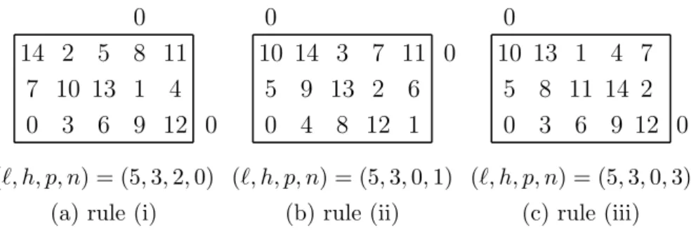
Chen and Hwang [3] gave a set of rules (CH-RULE in short) to determine the parameters `, h, p, n for a degenerate L-shape. Their rules always set ` to the width and h to the height of the rectangle (the degenerate L-shape). We now briefly describe their rules. CHEN-HWANG-RULE.
(i) Suppose hb 6≡ `a ≡ 0 (mod N). Let the zero immediately above the L-shape occurs at column j. Then
p = ` − j, n = 0.
(ii) Suppose `a 6≡ hb ≡ 0 (mod N). Let the zero immediately to the right of the L-shape occurs at row i. Then
p = 0, n = h − i.
(iii) Suppose `a ≡ hb ≡ 0 (mod N). If h > `, follow rule (i); otherwise, follow rule (ii). End-of-CHEN-HWANG-RULE.
The `, h, p, n chosen by CH-RULE satisfy the basic congruence equations in (3.2). Fig. 3 illustrates these rules.
0 3 6 9 12 7 10 13 1 4 14 2 5 8 11 0 0 (`, h, p, n) = (5, 3, 2, 0) (a) rule (i)
0 4 8 12 1 5 9 13 2 6 10 14 3 7 11 0 0 (`, h, p, n) = (5, 3, 0, 1) (b) rule (ii) 0 3 6 9 12 0 5 8 11 14 2 10 13 1 4 7 0 (`, h, p, n) = (5, 3, 0, 3) (c) rule (iii)
Figure 3: The (`, h, p, n) determined by CH-RULE.
W now characterize the (`, h, p, n) obtained by CH-RULE when DL(N; a, b) has a degenerate L-shape.
Theorem 10 If DL(N; a, b) satisfies
(C1), then CH-RULE derives an L-shape of shape (S2) with (`, h, p, n) = (N0, d, i, 0);
(C2), then CH-RULE derives an L-shape of shape (S3) with (`, h, p, n) = (d0,N
d0, 0, j); (C3), then CH-RULE derives an L-shape of shape
(S6) with (`, h, p, n) = (d0, d, 0, d) if d < d0;
(S5) with (`, h, p, n) = (d0, d, d0, 0) if d > d0.
Proof. First, suppose DL(N; a, b) satisfies (C1). Then there exists 1 ≤ i ≤ min{d, N0−
1} such that db ≡ ia (mod N). By Theorem 2, ` = N0, h = d; also, (C1) ⇒ (1). So
hb 6≡ `a ≡ 0 (mod N). Let the zero immediately above the L-shape occurs at column j. Since `a ≡ 0 (mod N), j = ` − i. So CH-RULE will follow rule (i) and will set p = `−j = i and set n = 0. Thus m = `−p = j > 0, n = 0, p = i > 0, q = h−n = h > 0; so the L-shape is of shape (S2).
Next, suppose DL(N; a, b) satisfies (C2). Then there exists 1 ≤ j ≤ min{d0,N
d0 − 1}
such that d0a ≡ jb (mod N). By Theorem 2, ` = d0 and h = N/d0; also, (C2) ⇒ (2).
So `a 6≡ hb ≡ 0 (mod N). Let the zero immediately to the right of L-shape occurs at row i. we have i = h − j. So CH-RULE will follow rule (ii) and will set p = 0 and set
n = h − i = j. Thus m = ` − p = ` > 0, n = j > 0, p = 0, q = h − n = N/d0− j > 0; so
the L-shape is of shape (S3).
Finally, suppose DL(N; a, b) satisfies (C3). By Theorem 2, (C3) ⇒ (Condition 3). So `a ≡ hb ≡ 0 (mod N). Let the zero immediately above the L-shape occurs at column
j and to the right of L-shape occurs at row i. Then i = j = 0. If d < d0, then h < `.
So CH-RULE will follow rule (ii) and will set p = 0 and set n = h − i = h = d. Thus m = ` − p = ` > 0, n = d > 0, p = 0, q = h − n = 0; so the L-shape is of shape (S6). If
d > d0, then h > `. So CH-RULE will follow rule (i) and will set p = ` − j = ` = d0 and
set n = 0. Thus m = ` − p = 0, n = 0, p = d0 > 0, q = h − n = d > 0; so the L-shape is
of shape (S5).
6
The relations between CH-ALGO and CH-RULE
Both CH-ALGO and CH-RULE determine the four parameters `, h, p, n for a degenerate L-shape. Unfortunately, the solution of (`, h, p, n) using CH-RULE [3] does not always coincide with the values given by the CH-ALGO. For the example in Fig. 3 (b), the solution of the CH-RULE is
(`, h, p, n) = (5, 3, 0, 1) and the solution of the CH-ALGO is
(`, h, p, n) = (5, 7, 5, 4) 16
(see Fig. 4). In this section, we will explain the relations between the two sets of solutions. 0 4 8 12 1 5 9 13 2 6 10 14 3 7 11 0 0 ` = 5 h = 7 p = 5 n = 4
Figure 4: An alternative representation of the L-shape in Fig. 3 (b).
From Theorem 9 and Theorem 10, we know that CH-ALGO will not derive an L-shape of shape (S4) or (S6) or (S7) and CH-RULE will not derive an L-shape of shape (S1) or (S4) or (S7). We now further explain the reason below. CH-ALGO will not derive an
L-shape of shape (S4) or (S6) because it always has q = h − n = dUu+1 > 0 (recall that
{Ui}k+1i=−1 is strictly increasing and U−1 = 0). Also, CH-ALGO will not derive an L-shape
of shape (S7) since if n = d(Uu + vUu+1) = 0, then u = −1 and v = 0 and therefore
p = su − (v + 1)su+1= s−1− s0 > 0, a contradiction to the assumption that the L-shape
is of shape (S7). CH-RULE will not derive an L-shape of shape (S1) or (S4) since it always sets ` to the width and h to the height of the degenerate L-shape. Also CH-RULE will not derive an L-shape of shape (S7) since it always has n and p not both zero. We now summarize the results of Theorem 9 and Theorem 10 in Table 1 and compare the degenerate shapes derived by CH-ALGO and CH-RULE in Table 2.
The following three corollaries follow from Theorem 9 and Theorem 10.
Corollary 11 CH-ALGO and CH-RULE derive the same shape when DL(N; a, b)
sat-isfies (C1), satsat-isfies (C2) and j ≥ N
2d0 or satisfies (C3) and d > d0. CH-ALGO and
CH-RULE derive different shapes when DL(N; a, b) satisfies (C2) and j < N
2d0 or satisfies
(C3) and d < d0.
Table 1: The shapes derived by CH-ALGO and CH-RULE.
shape S1 S2 S3 S4 S5 S6 S7
CH-ALGO v v v v
CH-RULE v v v v
Table 2: The comparison between CH-ALGO and CH-RULE.
condition C1 C2 C3
j < N
2d0 j ≥ 2dN0 d < d0 d > d0
CH-ALGO S2 S1 S3 S1 S5
CH-RULE S2 S3 S3 S6 S5
consistent yes no yes no yes
Let (ˆ`, ˆh, ˆp, ˆn) denote the solution of ALGO and ( ˙`, ˙h, ˙p, ˙n), the solution of
CH-RULE. Corollary 12 and Corollary 13 show that when the two sets of solutions are differ-ent, one can be obtained from the other.
Corollary 12 If DL(N; a, b) satisfies (C2) and j < N
2d0, then ˆ ` = ˆp = ˙`, ˆh = ˙n + & ˙` − ˙n ˙h ' ˙h, ˆn = ˙n + ( & ˙` − ˙n ˙h ' − 1) ˙h, and ˙` = ˆ`, ˙h = ˆh − ˆn, ˙p = 0, ˙n = j.
Corollary 13 If DL(N; a, b) satisfies (C3) and d < d0, then
ˆ ` = ˆp = ˙`, ˆh = & ˙` ˙h ' ˙h, ˆn = ( & ˙` ˙h ' − 1) ˙h, and ˙` = ˆ`, ˙h = ˙n = ˆh − ˆn, ˙p = 0. 18
References
[1] R. C. Chan, C. Y. Chen, and Z. X. Hong, “A simple algorithm to find the steps of double-loop networks,” Discrete Appl. Math. 121 (2002), 61-72.
[2] C. Y. Chen and F. K. Hwang, “The minimum distance diagram of double-loop net-works,” IEEE Trans. Comput. 49 (2000), 977-979.
[3] C. Y. Chen and F. K. Hwang, “Equivalent L-shapes of double-loop networks for the degenerate case,” Journal of Interconnection Networks 1 (2000), 47-60.
[4] Y. Cheng and F. K. Hwang, “Diameters of weighted double loop networks,” J. Al-gorithms 9 (1988), 401-410.
[5] M. A. Fiol, J. L. A. Yebra, I. Alegre, and M. Valero, “A discrete optimization problem in local networks and data alignment,” IEEE Trans. Comput. C-36 (1987), 702-713. [6] F. K. Hwang, “A complementary survey on double-loop networks,” Theoret. Comput.
Sci. 263 (2001), 211-229.
[7] F. K. Hwang and W. W. Li,“Reliabilities of double-loop networks,” Probability in the Engineering and Informational Sciences 5 (1991), 255-272.
[8] C. K. Wong and D. Coppersmith, “A combinatorial problem related to multimodule organizations,” J. Assoc. Comput. Mach. 21 (1974), 392-402.