針對壓縮視訊之畫面解析度改善

國

立

交

通

大

學

電子工程學系電子研究所碩士班

碩

士

論

文

針對壓縮視訊之畫面解析度改善

Spatial Resolution Enhancement

for Compressed Videos

指導教授：王聖智 博士

研 究 生：吳宗翰

針對壓縮視訊之畫面解析度改善

Spatial Resolution Enhancement for Compressed Videos

研 究 生: 吳宗翰

S t u d e n t: Tsung-Han Wu

指導教授: 王聖智

A d v i s o r: Shengjyh Wang

國 立 交 通 大 學

電子工程學系電子研究所碩士班

碩 士 論 文

A Thesis Submitted to Department of Electronics Engineering & Institute of Electronics National Chiao Tung University in partial Fulfillment of the Requirements for the Degree of Master in

Electronics Engineering

June 2006

HsinChu, Taiwan, Republic of China 中華民國九十五年六月

針對壓縮視訊之畫面解析度改善

研究生: 吳宗翰

指導教授: 王聖智 博士

國立交通大學

電子工程學系 電子研究所碩士班

摘要

在本文中，我們首先實作了一個針對壓縮視訊（像是 H.264/AVC）之畫面解析度改善 的方法。接著，我們分析這個方法的模擬結果。我們在模擬結果裡面發現這個畫面解析度 改善方法的幾樣缺點，像是模擬結果裡出現的一些瑕疵(artifacts)，還有場景變換(scene change)及快速運動(fast motion)所造成的一些問題。因此，我們提出了兩個方法去壓抑這些 瑕疵的出現，一個是空間域的中位數正則項(median regularization term)，一個是時間軸的中 位數濾波器(median filter)。為了克服場景變換及快速運動在先前的超解析度(super-resolution) 演算法裡所造成的問題，我們提出了兩個方法，一個是全域性的方法(global method)，一個 是區域性的方法(local method)。加入這些修改後，先前方法遇到的瑕疵及問題，明顯獲得改 善。

Spatial Resolution Enhancement for Compressed Videos

Student:

Tsung-Han Wu

Advisor:

Dr.

Shengjyh Wang

Institute of Electronics

National Chiao Tung University

Abstract

In this thesis, we first implement a spatial resolution enhancement algorithm for H.264/AVC compressed videos. Based on the analysis of the simulation results, we identify a few shortcomings of this algorithm, like some visual artifacts in the enhanced videos and some problems caused by scene change and fast motion. Then, we propose two methods to suppress these artifacts, including adding a median regularization term in the spatial-domain and using a median filter in the temporal domain. We also propose two methods, a global method and a local method, to overcome the scene change and fast motion problems. With these modifications, the artifacts and problems are suppressed significantly.

誌謝

能夠順利完成碩士論文，首先最感謝的是我的指導教授 王聖智老師，在

研究的過程中給予我充分的信任與空間，讓我能夠自由的發揮；在遭遇問題及

挫折時，也能給予我適當的建議及鼓勵。除了學術方面的指導外，老師也教導

我很多做人處事的方法及態度，在各方面都是我應該好好學習的對象。當然也

要感謝實驗室的伙伴們，我會永遠記得跟你們一起打拼的日子。還有要感謝的

是我的家人們，有你們在背後的支持才能讓我繼續走下去。最後，要感謝的是

我的女朋友紹萱，這段日子裡的陪伴與支持，讓我能度過辛苦的研究過程。

Content

摘要... i Abstract ... ii 誌謝... iii Content ... iv List of Figures... vi List of Tables ... ix Chapter 1 Introduction... 1 Chapter 2 Background... 2 2.1 Introduction to H.264/AVC ... 2 2.1.1 H.264/AVC Codec ... 2

2.1.1.1 The H.264/AVC Encoder... 2

2.1.1.2 The H.264/AVC Decoder... 4

2.1.2 H.264/AVC Structure... 4

2.1.2.1 The Baseline Profile... 6

2.1.2.2 The Main Profile... 9

2.1.2.3 The Extended Profile...11

2.1.2.4 The FRExt Profile... 12

2.2 Super-Resolution Methods for Compressed Video ... 14

2.2.1 System Model... 14 2.2.2 Quantizers... 16 2.2.3 Motion Vectors ... 18 2.2.4 Compression Artifacts ... 19 2.2.4.1 Artifact Types... 19 2.2.4.2 Suppression of Artifacts ... 19 2.2.5 Super-Resolution Methods ... 21

2.2.5.1 Projection onto Convex Set Methods... 21

2.2.5.2 Stochastic Methods ... 22

2.2.5.3 Hybrid Methods... 23

Chapter 3 Spatial Resolution Enhancement on Compressed Videos ... 24

3.1 System Model... 24

3.1.1 Video Acquisition ... 24

3.1.2 Video Compression... 25

3.2 Spatial-Domain MAP Estimator for Super-Resolution ... 29 3.2.1 Fidelity Constraint ... 29 3.2.1.1 Motion Warping... 29 3.2.1.2 Blur ... 31 3.2.2 Prior Model... 32 3.2.3 Optimization Procedure... 34 3.3 Proposed Modifications... 40 3.3.1 Artifact Reduction ... 40

3.3.2 Scene Change and Fast Motion Detection... 45

3.3.2.1 Global Method ... 45

3.3.2.2 Local Method ... 48

3.4 Overall Procedure... 58

Chapter 4 Experimental Results ... 60

4.1 4× Zooming ... 60

4.2 16× Zooming ... 74

Chapter 5 Conclusions... 84

List of Figures

Fig 2.1 Scope of H.264/AVC standardization[2]... 2

Fig 2.2 Structure of H.264/AVC [2]... 3

Fig 2.3 H.264 Encoder [4]... 3

Fig 2.4 H.264 Decoder [4]... 4

Fig 2.5 H.264 Baseline, Main, and Extended profiles [4]... 5

Fig 2.6 H.264 FRExt profiles [6]... 5

Fig 2.7 Subdivision of a picture into slices [2]... 6

Fig 2.8 Subdivision of a picture into slices using FMO [2] ... 6

Fig 2.9 Nine prediction modes [4]... 7

Fig 2.10 Segmentations of macroblock for motion compensation [2] ... 8

Fig 2.11 Performance of the deblocking filter for highly compressed pictures [4]... 9

Fig 2.12 Reference pictures from (a) past / future; (b) past; (c) future [4]... 10

Fig 2.13 Progressive and interlaced frames [2] ... 10

Fig 2.14 Conversion of a frame macroblock pair into a field macroblock pair [2]...11

Fig 2.15 Illustration of SP and SI-slices[4] ... 12

Fig 2.16 Left: Samples used for 8×8 spatial luma prediction; Right: Directions of spatial luma prediction modes [5] ... 13

Fig 2.17 SR methods may be used ... 14

Fig 3.1 Video acquisition process... 25

Fig 3.2 Video encoder... 25

Fig 3.3 Video decoder... 25

Fig 3.4 Relationship between Frame i and other frames ... 30

Fig 3.5 Illustration of the HBM algorithm [13]... 30

Fig 3.6 Frequency response of a Gaussian low-pass filter with different standard deviations .... 32

Fig 3.7 Simulation of denoising using different regularization methods [14]... 33

Fig 3.8 Flow chart of the resolution enhancement algorithm... 36

Fig 3.9 Resolution enhancement simulation of the Mobile sequence. ... 37

Fig 3.10 Resolution enhancement simulation of Stefan sequence. ... 38

Fig 3.11 Resolution enhancement simulation of News sequence... 38

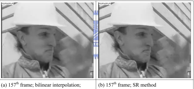
Fig 3.12 Resolution enhancement simulation of Foreman sequence. ... 38

Fig 3.13 PSNR performance: bilinear v.s. our method... 39

Fig 3.14 Pepper and salt noise in the reconstructed image of the Mobile sequence ... 40

Fig 3.17 Simulation result of resolution enhancement with artifact reduction: Stefan ... 42

Fig 3.18 Simulation result of resolution enhancement with artifact reduction: News ... 43

Fig 3.19 Simulation result of resolution enhancement with artifact reduction: Foreman ... 43

Fig 3.20 PSNR performance: bilinear v.s. our method with artifact reduction ... 44

Fig 3.21 The flowchart of the global method ... 45

Fig 3.22 Example of frame difference MAD ... 46

Fig 3.23 PSNR performance: bilinear v.s. our method with artifact reduction and global SC/FM detection ... 47

Fig 3.24 The flowchart of local method ... 48

Fig 3.25 Example of SC/FM region ... 49

Fig 3.26 Distribution of the difference in Fig 3.24(d)... 50

Fig 3.27 Flowchart of the local SC/FM detection method ... 52

Fig 3.28 SC/FM region detection results for News: i = 150 ... 53

Fig 3.29 SC/FM region detection results for Foreman: i = 157 ... 53

Fig 3.30 SC/FM region detection results for Stefan: i = 184 ... 54

Fig 3.31 Simulation result of SR method with artifacts reduction and local SC/FM detection : Mobile... 55

Fig 3.32 Simulation result of SR method with artifacts reduction and local SC/FM detection : Stefan... 55

Fig 3.33 Simulation result of SR method with artifacts reduction and local SC/FM detection : News ... 56

Fig 3.34 Simulation result of SR method with artifacts reduction and local SC/FM detection : Foreman... 56

Fig 3.35 PSNR performance: bilinear v.s. our method with artifact reduction and local SC/FM detection ... 57

Fig 3.36 Flow chart of the modified resolution enhancement algorithm ... 59

Fig 4.1 Simulation results with zooming ratio = 4, QP22: Mobile ... 61

Fig 4.2 PSNR with zooming ratio = 4, QP22: Mobile ... 61

Fig 4.3 Simulation results with zooming ratio = 4, QP28: Mobile ... 62

Fig 4.4 PSNR with zooming ratio = 4, QP28: Mobile ... 63

Fig 4.5 Simulation results with zooming ratio = 4, QP34: Mobile ... 64

Fig 4.6 PSNR with zooming ratio = 4, QP34: Mobile ... 64

Fig 4.7 Simulation results with zooming ratio = 4, QP22: Stefan... 65

Fig 4.8 PSNR with zooming ratio = 4, QP22: Stefan... 66

Fig 4.9 Simulation results with zooming ratio = 4, QP28: Stefan... 67

Fig 4.10 PSNR with zooming ratio = 4, QP28: Stefan... 67

Fig 4.11 Simulation results with zooming ratio = 4, QP34: Stefan... 68

Fig 4.13 Simulation results with zooming ratio = 4, QP22: News... 70

Fig 4.14 PSNR with zooming ratio = 4, QP22: News... 70

Fig 4.15 Simulation results with zooming ratio = 4, QP28: News... 71

Fig 4.16 PSNR with zooming ratio = 4, QP28: News... 72

Fig 4.17 Simulation results with zooming ratio = 4, QP34: News... 73

Fig 4.18 PSNR with zooming ratio = 4, QP34: News... 73

Fig 4.19 Simulation results with zooming ratio = 16, QP22: Mobile ... 75

Fig 4.20 Simulation results with zooming ratio = 16, QP28: Mobile ... 76

Fig 4.21 Simulation results with zooming ratio = 16, QP34: Mobile ... 77

Fig 4.22 Simulation results with zooming ratio = 16, QP22: Stefan... 78

Fig 4.23 Simulation results with zooming ratio = 16, QP28: Stefan... 79

Fig 4.24 Simulation results with zooming ratio = 16, QP34: Stefan... 80

Fig 4.25 Simulation results with zooming ratio = 16, QP22: News... 81

Fig 4.26 Simulation results with zooming ratio = 16, QP28: News... 82

List of Tables

Table 3.1 Parameter settings of super-resolution... 37

Table3.3 Parameter settings of hierarchical block matching... 37

Table 4.1 Parameter settings of super-resolution... 60

Table 4.2 Parameter settings of hierarchical block matching... 60

Table 4.5 Parameter settings of super-resolution... 74

Chapter 1 Introduction

H.264/AVC video coding is a high-coding-efficiency video coding standard [1]. It is based on the framework of block-based motion compensation and transform coding. This new H.264/AVC standard improves the coding efficiency through the adding of new features and functionality. From time to time, due to the constraints of channel bandwidth, storage size, and acquisition devices, the acquired video sequences are compressed into low-resolution videos. In order to improve the video quality, a resolution enhancement algorithm could be very helpful.

Multiframe resolution enhancement (“Super-Resolution”) techniques try to recover high-resolution images by exploring the useful information that is available in a sequence of low-resolution images. Super-resolution method has many applications, including the enhancement of medical images and surveillance videos. However, even though many methods have already been proposed to enhance non-compressed videos, only a few methods have been specially designed for compressed videos.

In this thesis, we propose a resolution enhancement method for compressed videos. This thesis is organized as follows. In Chapter 2, we describe the H.264/AVC coding standard and introduce a few super-resolution (SR) methods for compressed videos. In Chapter 3, we give a detail introduction to our resolution enhancement scheme and the proposed modifications for artifact reduction and quality improvement. Chapter 4 shows some simulation results. Finally, we give conclusions in Chapter 5.

Chapter 2 Background

In this chapter, we’ll first introduce the H.264/AVC[1] video coding standard. Then, we’ll introduce several super-resolution techniques for compressed video sequences.

2.1 Introduction to H.264/AVC

H.264/AVC, the ITU-T Recommendation H.264 and ISO/IEC International Standard 14496-10 Advance Video coding (AVC), is the newest video coding standard. The main contributions of H.264/AVC are the extremely high coding efficiency and the network-friendly video representation. The coding structure of this standard is similar to that of prior video coding standards, like H.261, MPEG-1, MPEG-2 / H.263, and MPEG-4 part 2. In the subsequent section, we will briefly introduce the H.264/AVC standard.

2.1.1 H.264/AVC Codec

As shown in Fig 2.1, the scope of the H.264/AVC standard only includes the decoder part to describe the bitstream syntax and the decoding process. This scope restriction provides the maximal freedom to the encoder for various kinds of applications.

Fig 2.1 Scope of H.264/AVC standardization[2]

2.1.1.1 The H.264/AVC Encoder

representation of the video and provides the header information in a manner appropriate for conveyance by a variety of transport layers or storage media, as shown in Fig 2.2.

Fig 2.2 Structure of H.264/AVC [2]

The functional elements of a compliant H.264/AVC encoder is shown in Fig 2.3. With the exception of the deblocking filter, most functional elements (prediction, transform, quantization, entropy encoding) are present in previous standards (MPEG-1, MPEG-2, MPEG-4, H.261, H.263). However, there exist some crucial changes in some of these functional blocks.

Fig 2.3 H.264 Encoder [4]

The Encoder includes two dataflow paths, a forward path (left to right) and a reconstruction path (right to left). During the forward path, an input frame/field Fn is processed in units of macroblock, and each macroblock is encoded in intra or inter mode. After the prediction process, the prediction P is subtracted from the current block to produce a residual (difference) block Dn. Then, Dn is transformed (using a block transform) and quantized to the coefficient X. This set of

decoding of the macroblock, is reordered and then entropy encoded. Finally, this compressed bitstream is passed to an NAL for transmission or storage.

During the reconstruction path, the encoder decodes the coefficient X to provide a reference picture for future predictions. There is a deblocking filter that is used to reduce blocking effects.

2.1.1.2 The H.264/AVC Decoder

The functional elements of a H.264/AVC decoder is shown in Fig 2.4. The dataflow path in the decoder is similar to the reconstruction path in the encoder. The decoder receives a bitstream from the NAL and decodes it to produce the residual block Dn’.

Using the header information decoded from the bitstream, the decoder creates a prediction block P, same as the prediction P in the encoder. Then P is added to Dn’ to produce uFn’, which is filtered to create the decoded block Fn’.

Fig 2.4 H.264 Decoder [4]

2.1.2 H.264/AVC Structure

H.264/AVC standard defines four different profiles: baseline profile, main profile, extended profile, and Fidelity Range Extensions (FRExt) profile. The Baseline Profile supports intra and inter-coding (I- and P-slices) and performs CAVLC (context-adaptive variable-length codes) [3] entropy coding. The Main Profile supports interlaced videos, inter-coding using B-slices, inter coding with weighted prediction, and entropy coding with context-based arithmetic coding (CABAC). The Extended Profile does not support interlaced videos nor CABAC, but adds modes

improve the capability of error resilience. Fig 2.5 shows the relationship among these three profiles.

Fig 2.5 H.264 Baseline, Main, and Extended profiles [4]

The FRExt Profile, the newest profile, supports 8×8 Intra Spatial Prediction, 8×8 Transform, and further extensions. As shown in Fig 2.6, it specifies a set of four new profiles, which are constructed as nested subsets of capabilities. The main difference between FRExt and non-FRExt H.264/MPEG4-AVC coding is the use of an 8x8 transform, in addition to the 4×4 transforms.

2.1.2.1 The Baseline Profile

The Baseline Profile supports I-slices and P-slices. In an I-slice, it contains only intra-coded macroblocks (MBs). On the other hand, a P-slice may contain intra-coded, inter-coded or skipped macroblocks.

2.1.2.1.1 Slices

Slices are sequences of macroblocks which are processed in the order of a raster scan. As shown in Fig 2.7, a frame may be split into one or several slices. Each slice can always be decoded correctly without the use of the data from other slices. However, when using deblocking filter across slice boundaries, it may need some information from other slices. In addition to the raster scan order of macroblocks in one slice, the Flexible Macroblcok Ordering (FMO) method can be used in H.264/AVC to partition a picture into several slice groups. Each slice group can be partitioned into one or more slices. Using FMO, a picture can be split into many scanning patterns of macroblock, as shown in Fig 2.8.

2.1.2.1.2 Intra Prediction

There are several intra prediction modes in H.264/AVC, mainly Intra 4x4 prediction and Intra 16x16 prediction modes. The Intra 4x4 mode predicts each 4x4 luma block separately and is well suited for the coding of texture parts in a picture. On the other hand, the Intra 16x16 mode predicts each 16x16 luma block separately and is suitable for the coding of smooth regions in a picture.

When doing intra prediction, the neighboring samples of previously-coded blocks, which are to the left and /or the top of the current block, are used. As shown in Fig 2.9, nine prediction modes can be used in the Intra 4x4 mode. The prediction modes in Intra 16x16 mode are similar to those in Intra 4x4 mode, but with only four prediction modes.

Fig 2.9 Nine prediction modes [4]

2.1.2.1.3 Inter Prediction

Inter prediction creates a prediction block from one or more previously encoded video frames or fields, by using block-based motion compensation. The main differences from previous coding standards are that H.264/AVC supports six different block sizes, as shown in Fig 2.10, and supports more accurate motion vectors (quarter-sample resolution in the luma component). For sub-sample motion compensation, the corresponding samples are obtained by using an interpolation process to generate sub-sampled image data.

Fig 2.10 Segmentations of macroblock for motion compensation [2]

2.1.2.1.4 Transformation and Quantization

Depending on the type of residual data that are to be coded, three different transformations can be used in H.264/AVC: a Hadamard transform for the 4×4 array of luma DC coefficients (Intra 16x16 prediction mode only); a Hadamard transform for the 2x2 array of chroma DC coefficients; and a DCT-based transform for all other 4 x4 blocks in the residual data.

H.264/AVC assumes a scalar quantizer. A quantization parameter (QP: 0~51) is used to determine the quantization step size of transform coefficients. Theses values are arranged so that an increase of 1 in the quantization parameter means a 12% increase of the quantization step size. An increase of step size by 12% also means a reduction of bit rate by approximately 12%

2.1.2.1.5 Deblocking Filter

The deblocking filter is used to reduce blocking effects in the decoded frame. It is applied after the inverse transform in the encoder/decoder. With this filter, H.264/AVC can further improve the coding efficiency because a filtered image is often a more faithful reconstruction of the original frame. After filtering, the subjective quality is significant improved, as shown in Fig 2.11.

(a) Without deblocking filter; (b) With deblocking filter

Fig 2.11 Performance of the deblocking filter for highly compressed pictures [4]

2.1.2.1.6 Entropy Coding

H.264/AVC supports two methods for entropy coding, Content Adaptive Variable Length Coding (CAVLC) and Content Adaptive Binary Arithmetic Coding (CABAC). In the Baseline Profile, CAVLC is adopted. In CAVLC, the VLC tables are designed to match the corresponding conditioned statistics, the entropy coding performance is better than the case when using a single VLC table only.

2.1.2.2 The Main Profile

2.1.2.2.1 B-slices

Each macroblock partition in a B-slice may be predicted from one or two reference pictures that are before or after the current picture in the temporal order. Depending on the reference pictures stored in the encoder/decoder, there are many options for the prediction references for a macroblock in a B-slice. Fig 2.12 shows three examples.

Fig 2.12 Reference pictures from (a) past / future; (b) past; (c) future [4]

2.1.2.2.2 Interlaced Video

In interlaced frames, whenever there is motion in the image, either caused by moving objects or caused by the camera movement, two adjacent rows tend to have a reduced degree of statistical dependency. In this case, it may be more efficient to compress the top field and the bottom field separately. Fig 2.13 shows the difference between progressive frames and interlaced frames. As field coding is used, the type of picture is signaled in the header of each slice. In the macroblock-adaptive frame/field (MB-AFF) coding mode, the coding type will be specified at the macroblock level. In this mode, the current slice is processed in units of 16 luminance samples wide and 32 luminance samples high. Each macroblock pair can be encoded as (a) two frame macroblocks or (b) two field macroblocks. The macroblock pair concept is illustrated in Fig 2.14.

Fig 2.14 Conversion of a frame macroblock pair into a field macroblock pair [2]

2.1.2.2.3 CABAC

The efficiency of entropy coding can be improved further if the Context-Adaptive Binary Arithmetic Coding (CABAC) is used. CABAC gets good compression performance by selecting probability models for each syntax element according to the element’s context, by adapting probability estimates based on local statistics, and by using arithmetic coding rather than variable-length coding. Compared to CAVLC, CABAC typically reduces the bit rate by 5%–15% [2].

2.1.2.3 The Extended Profile

2.1.2.3.1 SP and SI slices

SP and SI slices are specially coded slices that enable efficient switching between video streams and enable efficient random access for video decoders. SP slices support switching between similar coded sequences without increasing the bitrate in I slices, as shown in Fig 2.15(a). SI slices can switch to I slice that allows an exact match in an SP slice for random access or error control, as shown in Fig 2.15(b).

(a) Switching stream using SP-slices; (b) switching stream using I-slices Fig 2.15 Illustration of SP and SI-slices[4]

2.1.2.3.2 Data Partition

The encoded bitstream that makes up a slice is placed in three separate data partitions and each contains a subset of the coded slice. Partition A contains the slice header for each macroblock in the slice, Partition B contains coded residual data for Intra- and SI slice macroblocks, and Partition C contains coded residual data for inter coded macroblocks. Each Partition can be placed in a separate NAL unit and may be transported separately.

If A is lost, the decoder cannot decode this slice. B and C can be made to be independently decodable. The property that a decoder may decode A and B only, or A and C only, lends flexibility in an error-prone environment.

2.1.2.4 The FRExt Profile

2.1.2.4.1 8x8 Intra Spatial Prediction

In the FRExt Profile [5], it supports an 8x8 intra spatial prediction mode in addition to the Intra 4x4 mode and Intra 16x16 mode. The Intra 8x8 mode is introduced by extending the concept of Intra 4x4 mode, as shown in Fig 2.16.

Fig 2.16 Left: Samples used for 8×8 spatial luma prediction; Right: Directions of spatial luma prediction modes [5]

2.1.2.4.2 8x8 Transform

For high-fidelity, the preservations of fine details and texture, which generally requires larger basis functions, become equally important. In order to achieve this goal, the FRExt Profile includes an 8x8 integer transform and allows the encoder to choose adaptively between the 4x4 and 8x8 transforms for luma samples on a macroblock level.

2.1.2.4.3 Further Extension

The FRExt Profile contains three more important tools to support for extended sample bit depth and monochrome, as well as 4:2:2 and 4:4:4 chroma formats.

(1) Encoder-specified scaling matrices for perceptual tuned, frequency-dependent quantization.

(2) A residual color transform consisting of a reversible inter-based color conversion from RGB to YCgCo color space. This transform is applied to residual data only.

(3) A lossless coding capability requiring only a relatively simple bypass of transform and de-quantization.

2.2 Super-Resolution Methods for Compressed Video

Super-resolution (SR) techniques have been used to construct high-resolution images/videos from low-resolution images/videos, as shown in Fig 2.17. Super-resolution algorithms construct high-resolution images by exploiting sub-pixel shifts in the low-resolution data. These shifts are introduced by motion in the sequence and these shifts can be used to reveal the high-resolution information in the low-resolution frames.

While many methods have been proposed to enhance raw videos, only a few have been proposed to operate for compressed videos. Of course, any algorithm that enhances uncompressed-video algorithms can be used for compressed videos if we can decompress the compressed videos first. However, this process discards some important information about the quantization effects in the compressed videos. In the subsequent section, we will briefly introduce the super-resolution techniques for compressed videos.

Fig 2.17 SR methods may be used to construct a high-resolution video from a low-resolution source video [6]

2.2.1 System Model

This subsection introduces the general image model for compressed videos. This model relates the original high-resolution images to the decoded low-resolution images. Derivation of the model begins by generating an intermediate image sequence according to

AHf

where g is an (MN) ×1 vector that represents the low-resolution image, f is a (PMPN)×1 vector that represents a (PM)×(PN) high-resolution image, A is an (MN)×(PMPN) matrix that realizes the down-sampling operation, and H is a (PMPN)×(PMPN) filtering matrix.

Using the relationship between low and high-resolution images in (2.1), the compressed observation becomes MC MC DCT DCTQ Q T AHF g g T g∧ − ∧ ₊ ∧ ⎥ ⎥ ⎦ ⎤ ⎢ ⎢ ⎣ ⎡ ⎥ ⎥ ⎦ ⎤ ⎢ ⎢ ⎣ ⎡ ⎟⎟ ⎠ ⎞ ⎜⎜ ⎝ ⎛ − = 1 * _{, (2.2)}

where g is the decoded low-resolution image; ∧ T_DCTand −1

DCT

T are the forward and inverse Block-DCT operators, respectively; Q and Q* are the quantization and de-quantization operators,

respectively; and MC

g∧ is the motion-compensated prediction of the current frame. If parts of the

image are encoded as intra-blocks, then the predicted values for that region are zero.

Now, the high-resolution images of a dynamic image sequence are coupled through the motion field according to

k k l l C f

f = _, , (2.3)

where f and _l f are (PMPN)_k ×1 vectors that denote the high-resolution images at the time instances l and k, respectively; and C_l,k is a (PMPN)×(PMPN) matrix that describes the motion vectors relating the pixels at Time k to the pixels at Time l. These motion vectors describe the

actual displacement between high-resolution frames.

Combining (2.2) and (2.3), we get the relationship between a high-resolution and compressed image sequence at different time instances:

MC l MC l k k l DCT DCT l T Q Q T AHC f g g g∧ − ∧ + ∧ ⎥ ⎥ ⎦ ⎤ ⎢ ⎢ ⎣ ⎡ ⎥ ⎥ ⎦ ⎤ ⎢ ⎢ ⎣ ⎡ ⎟⎟ ⎠ ⎞ ⎜⎜ ⎝ ⎛ − = 1 * _{, , (2.4)}

⎟⎟ ⎠ ⎞ ⎜⎜ ⎝ ⎛ − = _{DCT lk k} ∧ MC_l l T AHC f g d _, , (2.5)

where g∧_l is the compressed frame at time l ,

MC l

g∧ is the motion-compensated prediction utilized in generating the compressed observation, and d is the DCT-domain residual coefficients. _l

2.2.2 Quantizers

We rewrite part of (2.4) by letting Q l

N , Q

l

n denote the errors introduced by quantization at the

time instance l in the DCT-domain and in the spatial domain, respectively. We also denote d~_l as the DCT-domain residual after quantization.

[ ]

[

]

Q l l l l Q Qd d N d~ = * = + _{, (2.6)} Q l MC l k k l MC l k k l DCT DCT

Q

Q

T

AHC

f

g

AHC

f

g

n

T

=

−

+

⎥

⎥

⎦

⎤

⎢

⎢

⎣

⎡

⎥

⎥

⎦

⎤

⎢

⎢

⎣

⎡

⎟⎟

⎠

⎞

⎜⎜

⎝

⎛

−

∧ ∧ − , , * 1 . (2.7)

Substituting (2.7) into (2.4), the relationship between a high-resolution image and the low-resolution observations becomes

Q l k k l l AHC f n g∧ = _, + . (2.8)

Now, the quantization procedure is treated as an additive noise process. The quantization is usually realized by dividing each transform coefficients by a quantization factor. The result is then rounded to the nearest integer. The transform coefficients can be reconstructed by the following relationship

( )

_{( )}

( )

_⎟⎟ ⎠ ⎞ ⎜⎜ ⎝ ⎛ ⋅ = ⎟ ⎠ ⎞ ⎜ ⎝ ⎛∧ i q i g T Round i q i g T DCT DCT , , , (2.8)

where T_DCT

( )

g, andi ⎟ ⎠ ⎞ ⎜ ⎝ ⎛∧ i g

T_DCT , denote the ith transform coefficient of the low-resolution image g and the decoded estimateg , respectively. q(i) is the quantization factor, and Round(· ) is an ∧

operator that maps each value to the nearest integer. From the above equations, we can see that Q

l

N is restricted to half of the quantization factor. Thus,

⎭ ⎬ ⎫ ⎩ ⎨ ⎧ _≤ ⎟ ⎠ ⎞ ⎜ ⎝ ⎛ ₋ ≤ − ∈ ∧ ∧ ∧ ∧ 2 2 : _, l l k k l DCT l k k q g f AHC T q f f . (2.9)

The equation (2.9) can be used as a constraint in some super-resolution techniques, like the Projection onto Convex Set (POCS) approach. This POCS approach is to be briefly described in the subsequent section.

In (2.6), we can treat Q l

N as a deterministic quantity that is defined as the difference between

l

d and d~_l. We may also treat Q

l

N as a stochastic vector for reconstruction. This stochastic vector can be modeled by various distributions [7]. For example, it can be modeled as a zero-mean independent identically distributed (I.I.D.) Gaussian random process, which leads to a mathematically tractable solution [8]. The noise model in the DCT-domain and the spatial-domain can be expressed as follow:

( ) ( ) ( )

⎭ ⎬ ⎫ ⎩ ⎨ ⎧− = − Q k Q k T Q k Q k N N Z N K N P 1 2 1 exp ) ( , and (2.10)

( ) (

) ( )

⎭ ⎬ ⎫ ⎩ ⎨ ⎧− = − − Q k DCT Q k DCT T Q k Q k N n Z n T K T n P 1 1 2 1 exp ) ( , (2.11) where Q k

K is the covariance matrix for Q k

N , and Z is the normalization factor.

After we have established the model of the quantization noise, we can use some stochastic approaches to estimate the high-resolution frames. We will introduce these methods in the

2.2.3 Motion Vectors

Incorporating the motion vectors into the super-resolution algorithm is also an important issue. Super-resolution techniques rely on sub-pixel relationships between frames in an image sequence. These SR techniques require an accurate estimate of the actual motion based on the observed low-resolution images. When a compressed bit-stream is available, the transmitted motion vectors provide additional information about the underlying motion. These vectors represent a degraded observation of the actual motion field and are generated by a motion estimation algorithm within the encoder. However, these motion vectors generated by the encoder may not be dense enough for super-resolution. Hence, in a super-resolution algorithm, it may be needed to re-estimate the true motion or improve the accuracy of the transmitted motion vectors. The latter one can be shown as follow,

( )

(

)

⎪⎭ ⎪ ⎬ ⎫ ⎪⎩ ⎪ ⎨ ⎧ − + − =

∑

− = 2 1 0 , , 2 , , argmin ˆ ˆ , ˆ , MN i Encoder k l T MV k l l k k l C k l AHC f g c i A C i C k l λ , (2.12)

where Cˆ is a matrix that represents the estimated motion field, _l,k c_l,k

( )

i is a two-dimensional vector that contains the motion vector for the pixel location i, Encoder

k l

C_, is a matrix that contains the motion vectors provided by the encoder,A

(

CEncoder i

)

k l T

MV , , produces an estimate for the motion at

pixel location i from the transmitted motion vectors, and λ quantifies the confidence in the transmitted information.

2.2.4 Compression Artifacts

2.2.4.1 Artifact Types

In video coding, several artifacts are commonly observed. They are listed below. (1) Blocking errors:

During the encoding process, images are divided into equally sized blocks and are transformed with a de-correlating operator, like the blockwise DCT transform. During the quantization of the DCT coefficients, blocking errors may be generated. Moreover, sometimes neighboring regions may be assigned with different quantization parameters even though these regions actually have similar visual contents. In this case, there could be some apparent artificial boundary in the decoded images.

(2) Temporal flickers:

Temporal flickers are attributed to an improper allocation of bits. In some applications, bits are distributed based on an assumption of future contents. If the assumption is inaccurate, the encoder may have to quickly adjust the amount of quantization to satisfy the rate constraint. In this case, the encoded video sequence possesses a temporally varying image quality. This phenomenon is called temporal flicker.

(3) Ringing artifacts:

Edges and impulsive features have high-frequency components. When utilizing a perceptually weighted quantization process, the encoder will preserve the low-frequency information more than the high-frequency information. Once if too many high-frequency components are lost, there could be some ringing artifacts in the decoded images.

2.2.4.2 Suppression of Artifacts

In super-resolution methods, some methods have been developed to attenuate compression artifacts. These techniques try to find a solution that may satisfy some predefined constraint while remain faithful to the observed data.

2.2.4.2.1 Constrained Least Square Method

In this method, a cost function is assigned to each type of artifact. The final reconstructed image can be found by minimizing the following cost function.

( )

2 3 2 2 2 1 2 ˆ ˆ _{Bp Rp p g}MC g p p E = − +λ +λ +λ − , (2.13)

where p is a vector representing the reconstructed image,gˆ is the estimate decoded from the

bit-stream, B and R are matrices that penalize the appearance of blocking and ringing artifects, respectively._gˆMC_{is the motion compensated prediction. λ}

1, λ2, and λ3 express the relative

importance of each constraint. Practically, B is implemented as a difference operator across block-boundaries and R is implemented as a high-pass filter within each block.

2.2.4.2.2 Projection onto Convex Set Method

In the framework, blocking and ringing artifacts are removed by defining a set of images that do not exhibit compression artifacts. For instance, the set of images that are smooth would not contain ringing artifacts and blocking artifacts. To define the set, the amount of smoothness must be quantified. Then, the solution is constrained by

{

g Bg TB

}

p∈ 2 ≤

: , (2.14)

where TB is the smoothness threshold used for the block boundaries and B is a difference operator

between blocks.

2.2.4.2.3 Maximum a Posteriori Method

In this frame work, we’ll use the idea of Baye’s rule. Thus the final reconstructed image is given by

(

) ( )

( )

g p p p p g p p _p ˆ | ˆ max arg = , (2.15) or

(

g p

)

p

( )

p p

2.2.5 Super-Resolution Methods

In this sub-section, we will introduce three commonly used methods in super resolution: the Projection onto Convex Set (POCS) method, the Maximum a posteriori (MAP) method, and the Maximum Likelihood (ML) method.

2.2.5.1 Projection onto Convex Set Methods

The POCS [9] method describes an iterative approach to incorporate prior knowledge about the solution into the reconstruction process. The incorporation of a priori knowledge into the solution can be interpreted as restricting the solution to be a member of a closed convex set Ci that are defined as a set of vectors satisfying a particular property. If the constraint sets have a nonempty intersection, then a solution that belongs to the intersection set m _i

i

S C

C =∩₌₁ , which is also a convex set, can be found by applying alternating projections onto these convex sets. Indeed, any solution in the intersection set is consistent with the a priori constraint and therefore is a feasible solution. We can use the recursion as following to get a vector belonging to the intersection. That is,

n m m n _{P P PPx} x 1 _{1 2 1} L − + _{= , (2.17)}

where x0 is an arbitrary starting point, and Pi is the projection operator which projects an arbitrary signal x onto the closed convex sets, C_i

(

i=1_Lm

)

.

As mentioned before, (2.9), (2.12), and (2.14) can be convex sets. The following example shows the projection operation that satisfies (2.9),

[ ]

( )

{

}

₍

₎

( )

{

}

₍

₎

⎪ ⎪ ⎪ ⎪ ⎩ ⎪ ⎪ ⎪ ⎪ ⎨ ⎧ − < − − − − > − + − − = − − otherwise f q g f AHC T AHC T q g T f AHC T T A H C f q g f AHC T AHC T q g T f AHC T T A H C f f P k l l k k l DCT k l DCT l l DCT k k l DCT DCT T T T k l k l l k k l DCT k l DCT l l DCT k k l DCT DCT T T T k l k k l , ˆ 5 . 0 ˆ ˆ , 5 . 0 ˆ ˆ ˆ 5 . 0 ˆ ˆ , 5 . 0 ˆ ˆ ˆ ˆ , 2 , , 1 , , 2 , , 1 ,

,

(2.18)

whereP ˆ_l

[ ]

f_k is the projection operator that accounts for the influence of the observationgˆ_lon the estimate of the high-resolution image fˆ_k.

The advantage of POCS method is its simplicity. It allows a convenient inclusion of a priori information. These methods have the disadvantages of non-unique solutions, slow convergence, and high computational cost.

2.2.5.2 Stochastic Methods

Stochastic SR image reconstruction, which is a Bayesian approach, provides a flexible and convenient way to model a priori knowledge concerning the solution.

Bayesian estimation methods are used when the a posteriori probability density function (PDF) of the original image can be established. The Maximum a posteriori (MAP) estimator of x maximizes the a posteriori PDF P(x|yk) with respect to x. That is,

(

x y y yp

)

P x=argmax | ₁, ₂,_L, . (2.19) Equivalently,

(

)

( )

{

P y y y x P x

}

x=argmax log ₁, ₂,_L, _p | +log . (2.20)

Both the a priori image model P(x) and the conditional density P

(

y₁,y₂,_L,y_p |x

)

will be defined by a priori knowledge concerning the high-resolution image x and the statistical information of noise. Since the MAP optimization in (2.20) includes a priori constraints

essentially, it provides regularized high-resolution estimates effectively.

The priori image can be modeled as different distributions. It can be model as a Gaussian random process[8], or a Markov random filed (MRF) priori[9]. Different priori models will have different effects on the reconstructed high-resolution images.

As mentioned in Section 2.2.2, (2.10) and (2.11) can be used as the conditional PDF for the MAP estimators in the DCT-domain[8] and spatial-domain[10], respectively.

Finally, we’ll introduce another stochastic method for super-resolution, the Maximum

likelihood (ML) estimator. The ML method is similar to the MAP method. It can be seen as a

special case of MAP estimation. The ML estimator maximizes the following conditional PDF

(

)

{

P y y y x

}

x=argmax log ₁, ₂,_L, _p | . (2.21)

An ML estimator does not use the prior term to regularized its estimation. Due to the ill-posed nature of super-resolution inverse problems, MAP methods are usually used in preference to ML methods.

Robustness and flexibility in modeling noise characteristics and a priori knowledge about the solution are the major advantage of the stochastic SR approach. Assuming that the noise process is white Gaussian, an MAP estimation with convex energy functions in the priors ensures the uniqueness of solution. Therefore, efficient gradient descent methods can be used to estimate the high-resolution images. It is also possible to estimate the motion information and the high-resolution images simultaneously.

2.2.5.3 Hybrid Methods

In above sub-sections, we have introduced the POCS estimator, the MAP estimator, and the ML estimator. It is possible to combine the POCS method with the ML (or MAP) method to get a hybrid estimator [11], [12]. The advantage of hybrid approach is that all a priori knowledge is effectively combined, and it ensures a single optimization solution in contrast to the POCS method.

Chapter 3

Spatial Resolution Enhancement on

Compressed Videos

In this chapter, we will first describe the system model used in this thesis. Then, we will discuss the spatial-domain MAP estimator for compressed videos. We will also describe the proposed modifications to overcome some problems. Finally, we will discuss the optimization procedure.

3.1 System Model

In this sub-section, we will first model the video acquisition, video compression, and noise. Then, we will formulate the super resolution problem.

3.1.1 Video Acquisition

The video acquisition process models the relationship between the continuous-time high-resolution images and discrete-time low-resolution images. The video acquisition process can be modeled as ) , ( ) , ; , ( ) , ( ) , (l k f n t h n t l k v l k g n r r d =

∑

+ , (3.1)

where n, l are the index of high-resolution images and low-resolution images respectively,g_d

( )

l, k

is the kth low-resolution (LR) image, f(n,t_r) is the high-resolution (HR) image at the reference time t_r, h(n,t_r;l,k) is the linear shift-varying blur mapping between the HR image and the kth LR image, and v( kl, ) is the acquisition noise. The video acquisition process can be depicted in Fig. 3.1.

Fig 3.1 Video acquisition process

3.1.2 Video Compression

The MPEG encoder and decoder can be generally expressed as Fig. 3.2 and Fig 3.3.

Fig 3.2 Video encoder

Fig 3.3 Video decoder

The LR image,g_d

( )

l, , as discussed before, will be encoded first in the encoder stage. The k

encoder will first perform motion compensation of this LR frame and we will get the prediction frameg_p

( )

l, . Then, the encoder will perform a series of block-DCTs to the difference frame of k

( )

l k

g_d , and g_p

( )

l, to produce the DCT coefficients k d

(

m,k

)

. The DCT coefficients d

(

m,k

)

are then quantized to produced the quantized DCT coefficients d_q

(

m, . We can expressed these k

)

(

)

{

( )

( )

}

( )

n t h

(

n t m k

)

G

(

m k

) (

V m k

)

f k l g k l g DCT k m d p n r DCT r p d , , , ; , , , , , + − = − =

∑

, (3.2)

(

)

{

(

)

}

(

)

(

) (

)

{

G m k G m k V m k

}

Q k m d Q k m d p q , , , , , + − = = , (3.3)

(

m k

)

DCT

{

g

( )

l k

}

G_p , = _p , , (3.4)

(

m k

)

DCT

{

v

( )

l k

}

V , = , , (3.5) and

(

)

=

∑

(

)

(

)

n r DCT r h n t m k t n f k m G , , , ; , , (3.6)

where m is the index in the DCT domain, and h_DCT

(

n,t_r;m,k

)

is the block-DCT of h(n,t_r;l,k). The quantized DCT coefficients d_q

(

m, and the corresponding step-sizes are available at k

)

the decoder. Thus, in the decoder stage, we can get the LR frames, y(l,k), by taking the block-IDCT and motion compensation. We can model the decoder stage as

( )

l k IDCT

{

d

(

m k

)

}

g

( )

l k

y , = _q , + _p , (3.7) In this thesis, we will only use the inter block search 8x8 and 8x8 block-DCT in the H.264/AVC encoder in the FRExt profile.

3.1.3 Noise Model

In this thesis, we assume that the compression is the major source of noise. This allows us to focus on integrating the compression stage into the super-resolution algorithm.

The quantization operator in (3.3) introduces the quantization noise in the DCT-domain. These errors correspond to the information discarded during quantization. We can express the

relationship between d

(

m,k

)

and d_q

(

m, as k

)

(

,

)

( , ) ) , (m k d m k n m k d_q = + _q−DCT , (3.8)

where )n_q−DCT(m,k is the quantization noise in the DCT-domain. Because we will perform the resolution enhancement in the spatial-domain, we have to express this noise in the spatial-domain. The quantization noise in the DCT domain and the spatial-domain is related as

{

( , )

}

) ,

(l k IDCT n m k

n_q−spatial = _q−DCT . (3.9)

The quantization noise in the spatial-domain is a linear combination of independent noise components in the DCT domain. Hence, by the Central Limit Theorem, the resulting noise process approaches the Gaussian distribution. Since we assume that the quantization noise is dominant, we can rewrite (3.7) as

( )

{

(

)

(

)

}

( )

( )

l k n k l t n h t n f k l g k m n k m d IDCT k l y spatial q n r r p DCT q , ) , ; , ( ) , ( , , , , − − + = + + =

∑

, (3.10) where

( )

(

_{q spatialk}

)

spatial q l k N K n ₋ , ~ 0, _{− ,} . (3.11) k spatial q

3.1.4 Problem Formulation

The system model in (3.10) is used for the formulation of an algorithm that reconstructs high-resolution frames from a sequence of low-resolution compressed frames. This approach is based on the assumption that information about a high-resolution frame may appear in multiple low-resolution observations. When the assumption is valid, then each low-resolution observation provides additional information about the high-resolution image frame.

Because of the flexibility and robustness of the Bayesian maximum a posteriori (MAP) approach, we choose this framework to construct our thesis. The spatial-domain MAP estimator for spatial resolution enhancement can be written as

( )

_{( )}

{

_{( ) ( ) ( )}

}

( r)

{

( ) ( )p ( r) ( r)

}

p r r t n f t n f k l y k l y t n f k l y k l y t n f t n f r p p p t n f , , | , , , , , , , , , | , , 1 1 max arg max arg , ˆ L L = = , (3.12)

where f ,ˆ

( )

n t_r is the estimate of the high-resolution image. With the use of the monotonic log function, the MAP estimator becomes

( )

n tr f(ntr)

{

py(lk) y( )lkp f(ntr) pf(ntr)

}

fˆ , argmax _, log _{, , , , | ,} log _,

1 +

3.2 Spatial-Domain MAP Estimator for

Super-Resolution

Obtaining a frame with enhanced resolution according to (3.13) requires definitions of the probability density functions (PDFs) _{( ) ( ) ( )}

r p f nt k l y k l y p _{, , , , | ,}

1 L and pf(n,tr). These PDFs incorporate

information about the compressed system, as well as a priori knowledge of the high-resolution images into the reconstruction framework. In this subsection, we will propose models for the PDFs and discuss the details of the MAP estimator.

3.2.1 Fidelity Constraint

The first term of (3.13) is called the fidelity constraint. From (3.11), the quantization noise process in the spatial domain is modeled as an additive Gaussian noise process. Thus, we can express this conditional PDF as follow by assuming y( )l,k1,L,y

( )

l,kp are independent

( ) ( ) ( )

( )

( )

⎭ ⎬ ⎫ ⎩ ⎨ ⎧ − − ∝ ⋅

∑

= p r p k k k r r t n f k l y k l y y l k H n t l k f n t p 1 1 2 , | , , , , L exp , ( , ; , ) ( , ) , (3.14) ( ) ( ) ( )

( )

∑

( )

= − − ∝ ⋅ p r p k k k r r t n f k l y k l y y l k H n t l k f n t p 1 1 2 , | , , , , , ( , ; , ) ( , ) log _L . (3.15)

Because H(n,t_r;l,k) in the fidelity constraint consists of motion warping, blurring, and compression stage, we have to discuss how to find the motion warping and how to define the blur in Fig 3.1.

3.2.1.1 Motion Warping

time index of reconstruction and observations at the time index of reference. As shown in Fig 3.4, if we want to reconstruct Frame i, we must find the relative motion between Frame i and other frames.

Fig 3.4 Relationship between Frame i and other frames

In order to find the relative motion between Frame i and other frames, we have to perform motion estimation. This step is a critical step in our approach. We need to choose an appropriate motion estimation method. Here, we adopt the Hierarchical Block Matching (HBM) algorithm [13] to do this motion estimation. This method is more suitable for super-resolution algorithm than other traditional block matching methods. The illustration of hierarchical block matching is shown in Fig 3.5.

The same block size is used at different levels. If we use an L-level HBM, then the block size NxN at Level l corresponds to the block size 2L-1Nx2L-1N at the full resolution. Because of this hierarchical structure, the HBM approach can catch more accurate object motions. After we have these accurate motion vectors, we can warp back the additional information from observations to the high-resolution frame that we want to reconstruct.

3.2.1.2 Blur

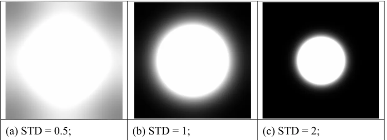
In the video acquisition process in Fig. 3.1, there are two kinds of blurs. One is from the sensor blur, while the other is from the nonzero aperture time. As we capture the image, we have no information about these two kinds of blurs. For simplicity, we use a simple spatial-domain Gaussian low-pass filter instead of estimating the accurate blur of the video acquisition process.

The standard deviation of the Gaussian low-pass filter can be chosen according to the zooming ratio. For a larger zooming ratio, we use a Gaussian low-pass filter with a larger standard deviation. For a smaller zooming ratio, we need a Gaussian low-pass filter with a smaller standard deviation.

This kind of choice can be explained in digital signal processing. For a larger zooming ratio, it seems the original high-resolution frame is downsampled more. Thus, there could be a serious aliasing effect in the low-resolution observations. Hence, we need a low-pass filter with a narrower bandwidth to suppress the aliasing effect. On the other hand, for a smaller zooming ratio, we can use a low-pass filter with a wider bandwidth. A Gaussian low-pass filter with a larger standard deviation in the spatial domain equals to a low-pass filter with a narrower bandwidth in frequency domain, and vice versa. This is why we can choose the standard deviation in this manner. The frequency response of Gaussian low-pass filter with different standard deviations are illustrated in Fig 3.6.

(a) STD = 0.5; (b) STD = 1; (c) STD = 2;

Fig 3.6 Frequency response of a Gaussian low-pass filter with different standard deviations

3.2.2 Prior Model

Now, we have to model the prior distribution _{( )}

( )

⋅

r

t n f

p _, , the second term of (3.13). This prior distribution is also called the regularization term. Because super resolution is always an ill-posed problem, it is very useful to include the regularization term to derive a stable solution. Moreover, the regularization term may also help the algorithm to remove artifacts and improve the speed of convergence. Here, we define the regularization term as

( )

f =−logpf

γ . (3.16)

We may model the prior distribution as a Gaussian random process, a Markov random field, or some other more complicated random processes. If we use the first-order Markov random field as the prior distribution, then it can be written as

( )

( )

⎪⎭ ⎪ ⎬ ⎫ ⎪⎩ ⎪ ⎨ ⎧ − − ∝ ⋅

∑

∈ 2 , ( , ) 4 1 ) , ( exp N i r r t n f f n t f i t p r , (3.17) and thus ( )

( )

2 , ₄ ( , ) 1 ) , ( log

∑

∈ − − ∝ ⋅ N i r r t n f f n t f i t p _r , (3.18)

where N means the four neighbor of the pixel at (n,tr). The RHS of (3.18) can also be seen as a

and an averaging intensities of its four neighbors. As the noise and edge pixels both contain high-frequency energy, they will be removed in the regularization process and the resulting image will not contain sharp edges.

In order to preserve edges and some other features, we may use other kinds of regularization terms. In [14], the author proposes a useful regularization method for denoising and deblurring, named the bilateral total variation method (BTV). The most useful property of the BTV method is that it tends to preserve edges in the reconstruction process. This regularization term can be written as

( )

(

)

( )

( )

, 0,0 1 0 1 ≤ < ≥ + − =

∑∑

− = = + _α α γ f t p f t S S f t l m p l p m r m y l x r l m r BTV , (3.19) where l x S , and m y

S shift f

( )

t_r by l, and m pixels in horizontal and vertical directions respectively, presenting several scales of derivatives. The scalar α is used to offer the spatial decaying effect to the summation of the regularization terms.

In a simple simulation, the author added Gaussian white noise with zero mean and variance 0.045 into the original image. Then, as shown in Fig. 3.7, we can easily compare the performance between the traditional regularization method (3.18) and the BTV method (3.19)

(a) Original; (b) Noisy; (c) Regularization using (3.18);

(d) Regularization using (3.19) with p = 2

Fig 3.7 Simulation of denoising using different regularization methods [14]

In Fig 3.7, we can see that the performance of the BTV method is much better than the traditional method. Hence, we choose the BTV method to be our prior.

3.2.3 Optimization Procedure

The first term and the second term in (3.13) are defined as (3.15) and (3.19) respectively. Hence, we can write the cost function of the spatial-domain MAP estimator as

( )

(

)

( )

BTV

(

( )

r

)

k k k r r r y k H t k f t f t t f E p γ λ⋅ + − =

∑

=1 2 ) ( ) ; ( , (3.20)

where y

( )

k , H( kt_r; ), and f(t_r) are y ,

( )

l k , H(n,t_r;l,k), and f(n,t_r), respectively. Here, we drop the spatial index l and n for simplicity and λ is the regularization parameter.

After we have the cost function, we can use any optimization method to find the optimized estimation of the high-resolution image, fˆ . Here, we adopt the steepest descent method to find the solution to this optimization problem:

( )

n n n f E f fˆ ₊₁ = ˆ −β ⊗∇ ˆ , (3.21)

( )

(

) ( )

[

(

)

]

BTV

( )

n k k k n r T r n H t k y k H t k f f f E p ˆ ˆ , , ˆ 1 γ λ⋅∇ + − − = ∇

∑

= , (3.22)

( )

_∑∑

[

]

(

)

− = = − − + _{− ⋅ − + ≥ < ≤} = ∇ p p l p m n m y l x n l x m y l m n BTV f I S S sign f S S f l m 0 1 0 , 0 , ˆ ˆ ˆ _{α α} γ , (3.23)

where β is a scalar matrix to define the step size in the direction of the gradient, and ⊗ is defined as the element multiplication.

The scalar matrix β may be fixed or adaptive. Here we use the information about the sign of the gradient in the nth iteration and the (n+1)th iteration to decide whether each scalar element in the matrix β should be larger or smaller. This adaptation method can be expressed as

( )

(

n

)

(

( )

n

)

n n

n β ω sign E f sign E f β

of the scalar matrix β_n+1. We can initially choose an starting valueβ₀, and then change the value of β adaptively at each iteration.

In (3.20), the regularization parameter λ is used to balance the contribution of the fidelity constraint and the regularization term. This parameter can be either fixed or adaptive. Since it could be a tedious work to choose the λ manually, we will use an adaptive way to decide the value of λ in each iteration. Based on the concept of [15], [16], we can also assume some properties for λ. Here, we assume

1. λ is proportional to the first-term in the RHS of (3.20).

2. λ is inversely proportional to the second-term in the RHS of (3.20). 3. λ is larger than zero.

Thus, we use a logarithmic type of regularization function to adapt the regularization parameter in each iteration. Here, we have

( )

( )

(

)

⎪ ⎪ ⎭ ⎪ ⎪ ⎬ ⎫ ⎪ ⎪ ⎩ ⎪ ⎪ ⎨ ⎧ + + − =

∑

= 1 ) ( ) ; ( log 1 2 ξ γ λ r BTV k k k r r n _{f t} t f k t H k y p , (3.25)

where ξ is used to prevent the denominator from becoming zero.

The optimization procedure of super resolution algorithm is illustrated in Fig 3.8 and is described as follows :

1. Choose an observation of a low-resolution image that is to be reconstructed; bilinearly interpolated it to get an initial estimate of the high-resolution image.

2. The relative motion between the frame to be reconstructed and other frame is estimated to get

) , ; , (n t l k H _r . 3. Calculate ∇E ˆ

( )

f .

6. Use (3.24) to update the step-size.

7. Repeat Steps 3 to 6 till the stop criterion is reached.

Fig 3.8 Flow chart of the resolution enhancement algorithm

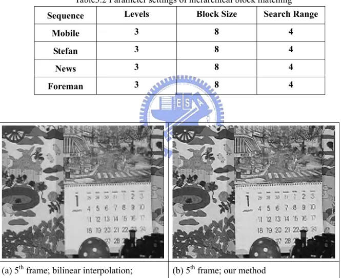
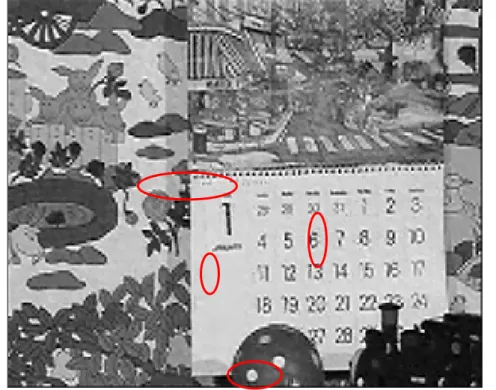
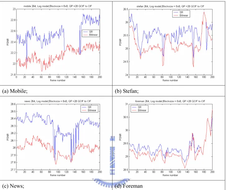
Some simulations using the above methods are shown below. The parameter settings of these simulations as shown in Table 3.1 and Table 3.2.

Table 3.1 Parameter settings of super-resolution

Sequence QP Size Ref. frame No. STD of Blur α m

Mobile 28 QCIF to CIF 4 0.5 1 2

Stefan 28 QCIF to CIF 4 0.5 1 2

News 28 QCIF to CIF 4 0.5 1 2

Foreman 28 QCIF to CIF 4 0.5 1 2

Table3.2 Parameter settings of hierarchical block matching

Sequence Levels Block Size Search Range

Mobile 3 8 4

Stefan 3 8 4

News 3 8 4

Foreman 3 8 4

(a) 5th frame; bilinear interpolation; (b) 5th frame; our method

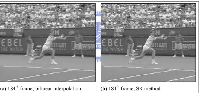
(a) 184th frame; bilinear interpolation; (b) 184th frame; our method

Fig 3.10 Resolution enhancement simulation of Stefan sequence.

(a) 150th _{frame; bilinear interpolation; (b) 150}th _{frame; our method;}

Fig 3.11 Resolution enhancement simulation of News sequence.