非重疊攝影機間之機率式交通流量建模方法

國

立

交

通

大

學

多媒體工程研究所

碩

士

論

文

非

重

疊

攝

影

機

間

之

機

率

式

交

通

流

量

建

模

方

法

Probabilistic Modeling of Dynamic Traffic Flow between

Non-Overlapping FOVs

研 究 生：邱維辰

指導教授：莊仁輝 教授

指導教授：王聖智 教授

非重疊攝影機間之機率式交通流量建模方法 Probabilistic Modeling of Dynamic Traffic Flow between

Non-Overlapping FOVs 研 究 生：邱維辰 Student：Wei-Chen Chiu 指導教授：莊仁輝 Advisor：Jen-Hui Chuang 指導教授：王聖智 Advisor：Sheng-Jyh Wang 國 立 交 通 大 學 多 媒 體 工 程 研 究 所 碩 士 論 文 A Thesis

Submitted to Institute of Multimedia Engineering College of Computer Science

National Chiao Tung University in partial Fulfillment of the Requirements

for the Degree of Master

in

Computer Science July 2009

Hsinchu, Taiwan, Republic of China

非重疊攝影機間之機率式交通流量建模方法 學生：邱維辰 指導教授：莊仁輝、王聖智 國立交通大學多媒體工程研究所碩士班 摘 要 在延伸現有視覺監視系統至全面性交通監控的過程中，如何推斷多 攝影機間之交通狀況是一項非常重要的課題。在本論文中，我們提出 一個於非重疊攝影機間之機率式交通流量建模的有效方法。基於物體 於攝影機間移動時其移動時間會符合某總體模型之假設，並藉由連續 估計此模型之參數，我們可以推斷出在不可視區域中之動態交通狀況。 原則上如果我們知道攝影機間之移動物體的對應關係，則移動時間的 總體模型的參數即可被估計出來。然而尋找物體間之對應關係在電腦 視覺領域中仍然是一個懸而未決的問題。在本文中，我們將非重疊攝 影機間物體對應關係之建立與總體移動時間模型之參數估計視為一個 統整性的最佳化問題，並利用期望值最大化演算法來反覆尋找最佳的 物體對應關係以及總體模型之參數解。在實際場景中的實驗結果證明 了我們的方法能有效地估計出總體移動時間模型之參數並準確推斷出 動態的交通情況。 關鍵字：交通流量，非重疊攝影機

Probabilistic Modeling of Dynamic Traffic Flow between Non-Overlapping FOVs

Student：Wei-Chen Chiu Advisors：Prof. Jen-Hui Chuang, Prof. Sheng-Jyh Wang

Institute of Multimedia Engineering National Chiao Tung University

ABSTRACT

The ability to infer the traffic status across multiple cameras allows the extended use of existing vision-based surveillance systems to global traffic monitoring. In this paper, we propose an efficient algorithm to probabilistically model the dynamic traffic flow between non-overlapping FOVs. By assuming the transition time of object moving across cameras follows a global model and consecutively estimate the model parameters, we may infer the time-varying traffic status in the unseen region. In principle, the parameters of the transition time model can be estimated if the object correspondence between non-overlapping FOVs is known. However, object correspondence itself is still an unsolved problem in computer vision. In this paper, we model object correspondence and the parameters estimation as a unified problem in a proposed Expectation-Maximization (EM) based framework. By treating object correspondence as a latent random variable, the proposed framework can iteratively search for the optimal object correspondence and model parameters. Experimental results on real data show the accuracy of dynamic model estimation and the beneficial inference of the traffic status.

誌謝 首先感謝我的指導教授，莊仁輝老師與王聖智老師。從大四預研生時 期進入實驗室，到碩士班結束，兩位老師不僅給予我許多研究方面的提點， 也在處事態度及人生經驗上讓我獲益良多。能夠順利的拿到碩士學位，實 在是因為有兩位老師的用心指導及包容。在此向辛苦的兩位老師致上最高 的敬意與感謝。另外也要感謝我的口試委員，陳永昇老師和林嘉文老師， 對這篇論文所提出的指導和建議。 接著要感謝實驗室的各位學長學弟們。尤其感謝敬群學長，從我大三 於國外交換學生階段開始就給予我研究領域上的啟蒙，其中經歷過工研院 實習及碩士班的研究期間，學長一直不吝於犧牲自己的時間與我討論，給 我很多的建議以及參考資料、學習方向，更分享了許多人生的歷練，這都 是我永遠無法忘記的，實是我生命中的貴人。很感謝慈澄學長、禎宇學長 及國華學長平時的照顧，以及一起在實驗室中打拚畢業的瑞男、文中、庭 瑋、世旻、聖中、永昌、尚一、宣良、邦展，大家的相互討論與分享，都 是我研究的助力。周節、瑋國、育瑋等學弟妹平時的諸多幫忙、已經畢業 的學長姐們的經驗傳承，更讓我在研究所期間助益良多。 最後感謝我的父母、家人對我的關懷、支持及鼓勵，感謝馨方的陪伴、 包容與體諒，你們都是我心理上最大的支柱。沒有你們，我或許無法堅持 到最後。感謝陪伴我走過學習歷程的眾多朋友與同學，我的一切都來自於 你們的貢獻，由衷感謝。

Contents

2.1 Surveillance systems with non–overlapping cameras . . . 9

2.2 Markov Chain Monte Carlo . . . 16

2.2.1 The Metropolis–Hastings algorithm . . . 17

2.2.2 The Gibbs sampler . . . 18

2.3 Expectation–Maximization . . . 20

3 Proposed Method 23 3.1 Selected Target . . . 23

3.2 Traffic Flow Model . . . 24

3.3 Problem Formulation . . . 26

3.4 Initialization . . . 33 4 Experiment and Results 36 5 Conclusion 45 Bibliography 46

List of Figures

1.1 A simple case: monitor traffic between two regions. . . 2

1.2 Overview of Dailey’s system. . . 3

1.3 A GPS–based AVLS for bus arrival time prediction. . . 3

1.4 Overview of Beymer’s system. . . 4

1.5 Results of Beymer’s system. . . 5

1.6 Flow diagram and result of Kim’s system. . . 6

1.7 An example of traffic surveillance system with non–overlapping cameras. . . 7

1.8 A simple interface of proposed system. . . 8

2.1 Two results of Javed’s work. . . 10

2.2 The framework of Song’s system. . . 11

2.3 An example of Rahimi’s work. . . 12

2.4 An example of Sheikh’s work. . . 14

2.5 An example of Makris’s work. . . 15

2.6 An counter example of Makris’s work. . . 16

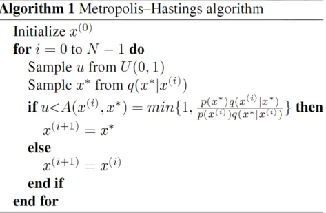
2.7 Metropolis–Hastings algorithm. . . 18

2.8 An example of Metropolis–Hastings algorithm . . . 19

2.9 Gibbs sampler. . . 20

3.1 The block diagram of the proposed system. . . 24

3.2 A result of target selection. . . 25

3.3 Some examples of distributions in the real life traffic. . . 26

3.4 Division the timeline of the day into overlapped time–windows. . . 26

3.5 The schematic diagram of xm, yn, cm(.), and tm. . . 28

3.6 Gibbs sampler in the proposed method. . . 29

3.7 A simple example of the Gibbs sampling. . . 30

3.8 A demonstration of the M step. . . 32

3.9 Proposed Expectation–Maximization algorithm. . . 32

3.10 Initialization of the EM algorithm for the first time–window. . . 33

3.11 A possible situation for the current time–window and the previous one. . . 34

3.12 Initialization of the EM for the following time–windows. . . 35

4.1 The experimental environment. . . 37

4.2 Divide the timeline into 34 overlapped time–windows in the experiment. . . 37

4.3 The transition–time distribution from time–window # 01 to time–window # 12. . . 38

4.4 The transition–time distribution from time–window # 13 to time–window # 24. . . 39

4.5 The transition–time distribution from time–window # 25 to time–window # 34. . . 40

4.6 Some results from applying the Tieu’s method to our experimental data. . . 41

4.7 Traffic flow state expressed by the average transition time. . . 43

4.8 Traffic flow state expressed by relative traffic changes. . . 43

4.9 Some transition–time distributions from the first example of different setting. . . 43

1 Introduction

With the rapid development of economy, the increasingly serious problem of traf-fic system is becoming one of the crucial factors for the growth of national econ-omy. As the urgent requirement of road using comes up, Intelligent Transport System (ITS) emerges to address the problems of road safety and congestion. ITS varies in the technologies applied, from basic management systems such as car navigation and traffic signal control system, to monitoring applications, such as security CCTV systems and to more advanced applications like prediction of transit vehicle arrival time. However, no matter what kind of application it is, the most commonly used quantity for the performance assessment of ITS is traffic flow. Hence, the modeling of traffic flow has become a key ingredient of ITS.

The traffic flow research has been widely discussed and studied for over 70 years. Among them, the development of traffic flow theory provides a tool to help transportation engineers understand and express the characteristics of traffic state. The basic idea of traffic flow theory is to model the microscopic and macroscopic relationships among traffic stream variables, including speed, flow and concen-tration (density). Many models have been proposed as analytical techniques such as traffic stream models including Greeshield’s model and Edie’s model, shock wave analysis, deterministic and stochastic queuing theories, and capacity analy-sis [1, 2, 3, 4]. Moreover, to make ITS more efficient, dynamic traffic flow model has gained popularity. The term “dynamic” here is to describe the traffic state changes caused by stochastic traffic flow uncertainties, such as traffic jams, acci-dents, weather condition, queue length in front of a traffic light, etc.

re-Figure 1.1: A simple case: monitor traffic between two regions.

gions, as shown in Figure 1.1. Given a vehicle moving from one region toward another, its traveling time may increase due to a heavy traffic state associated with an accident or traffic jam, or decrease in off–peak hours or due to other phenom-ena associated with smooth traffic flow. Hence, instead of using lots of variables to model the traffic flow, we can infer the traffic state by observing the “delay times” or “transition time” of objects moving across different regions.

Inspired by this intuitive idea, many research works and applications focus on dealing with the relevant problem of “delay times.” For example, in [5] and [6] Francesco Viti et al. claimed that the transition time of vehicles in urban networks is determined half by the driving time and half by the delay at intersections that mainly depends on the arrival time, queue length and the signal frequency. Hence, they proposed a probabilistic model for delay times at controlled intersection. In addition, another major topic of ITS about the prediction of transit vehicle arrival time is also based on the concept of the delay modeling. In [7, 8, 9, 10], Dailey et al. presented an algorithm to predict transit vehicle arrival time by using an

Figure 1.2: Overview of Dailey’s System [8].

Figure 1.3: A GPS–based AVLS for bus arrival time prediction.

location pairs. The data are used with historical statistics in an optimal filtering framework to predict future arrivals. An overview of their system is shown in Figure 1.2.

There are still lots of methods trying to provide an accurate prediction of transit vehicle arrival times. For instance, in [11], Steven et al. used artificial neu-ral networks (ANNS) trained with historical AVLS data to do dynamic prediction; in [12], the authors used support vector machines (SVM) instead. An example of GPS–based AVLS for bus arrival time prediction is illustrated in Figure 1.3.

However, all the methods mentioned above suffers from drawbacks of being expensive in installation and maintenance because they are highly dependent upon

Figure 1.4: Overview of Beymer’s system [15].

AVLS, which generally costs a lot. Besides, due to the privacy issue, promoting those AVLS–based applications is not as easy as it appears. Fortunately, in recent years, as a result of rising demand for security, many surveillance cameras have been installed in major intersections and some regions of interest, and the number of cameras is growing rapidly. This trend enables the development of another form of ITS technologies – “vision–based traffic surveillance system.” This kind of system has the features of relatively low installation cost, easy operation and less traffic disruption during maintenance in contrast to AVLS [13, 14].

Actually, many image processing and computer vision techniques for the analysis of traffic flow video sequences have been widely used for road traffic monitoring and traffic data collection. Considerable amount of improvements have also been made [14]. For example, in [15, 16] Beymer et al. developed a feature based tracking approach for the task of tracking vehicle under conges-tion. By tracking individual vehicles, the system can measure conventional traffic

(a) (b)

Figure 1.5: Results of Beymer’s system [15]. (a) Sample feature tracks. (b) Sample feature groups.

Figure 1.4 shows an overview of their system. Some results are shown in Fig-ure 1.5. In [17], the authors used probabilistic line featFig-ure grouping algorithm to perform model–based 3–D vehicle detection and description. With the tracking algorithm based on the zero–mean correlation matching, their approach provides a method for vehicles monitoring. The flow diagram and a result of their system are shown in Figure 1.6.

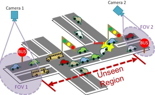
Nevertheless, almost all existing vision–based traffic surveillance systems are constrained by cameras’ field of views (FOVs). Moreover, these systems only concern about the visible information in the video sequences and only indicate the “local” traffic status at the camera location. However, for a camera surveil-lance system that covers a wide area, it is not always possible to have overlapping views; the observed regions can be widely separated in time and space. As shown in Figure 1.7, cameras only have “local ”information from their FOVs. Without the traffic status in the unseen region between non–overlapping cameras, we can-not infer a “global” traffic flow. Hence, under the condition that most existing cameras’ FOVs are non–overlapping, if we want to build a practical vision–based wide–area surveillance system for traffic flow monitoring, we have to estimate the

(a)

(b)

Figure 1.6: (a) Flow diagram of Kim’s system. (b) An example tracking result [17].

traffic state in the unseen regions between FOVs.

In this thesis, our main objective is to extend existing vision–based surveil-lance systems from local–range monitoring toward global–range monitoring of traffic flow by inferring the traffic state between non–overlapping FOVs. The key barrier we will meet is having no visual information of the road, which links the non–overlapping FOVs, to observe the traffic state directly. In general, if we can identify the same vehicle across cameras (e.g., using license plate recognition), it will be easy to achieve our objective. However, there is no guarantee that we can always achieve the correspondences of objects across cameras. Hence, instead of solving the problem by identifying the same vehicle across cameras, here we propose a different method.

Figure 1.7: An example of traffic surveillance system with non–overlapping cameras.

the prior knowledge of the global transition–time distribution, we may infer the rough correspondence among our targets. Unfortunately, that prior knowledge is not available in this problem. From another point of view, every correspon-dence of vehicles can be treated as an observation from the global transition–time model. By collecting these observations of correspondence, we can derive the global model. Again, we do not have any information about correspondences. Hence, in our system, we exploit the physical dependence between the corre-spondences of buses and the global transition–time distribution, and formulate the object correspondence and the parameters estimation for the transition–time distribution as a unified problem in a proposed Expectation–Maximization (EM) based framework. By treating object correspondence as a latent random variable, the optimized solution can be found through iterations.

As for, the transition–time model, since it may might vary with time due to dynamic changes of traffic state, a sequential EM are used to adapt to such changes over time. A simple interface of our system is shown in Figure 1.8. Such

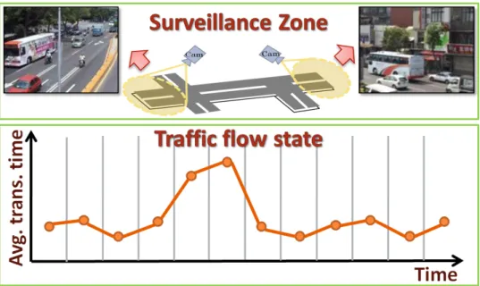
Figure 1.8: A simple interface of proposed system. It provides the information of the time–variant traffic state between non–overlapping FOVs.

a system can also be combined with the map services, such as Google Map or the CCTV Live–cam service on some important traffic spots, so that users can fetch the current traffic state from the Internet.

This thesis is organized as follows. In Chapter 2, we will first introduce some related works and mathematical techniques. In Chapter 3, we will present the proposed algorithm for modeling the dynamic changes of traffic state between non–overlapping FOVs. Some experimental results are shown in Chapter 4. Fi-nally, we give our conclusion in Chapter 5.

2 Related Work

In this chapter, we will first introduce a few related researches on surveillance sys-tems with non–overlapping cameras. Since in the proposed method we use some mathematical techniques such as Monte Carlo Markov Chain and Expectation– Maximization, we will also give some brief introductions of these mathematical techniques.

2.1

Surveillance systems with non–overlapping cameras

In general, the key problem of surveillance systems with non–overlapping cam-eras is to build the relationships between objects moving through different FOVs, i.e., the association of objects across cameras. Once the association is established for all objects, problems such as co–operative object tracking, object counting, and monitoring of objects activities become easier to resolve.

In [18, 19], Javed et al. proposed a method to establish the correspondence between observations across cameras. During a training phase, they manually es-tablished the correspondence to discover the relationships between cameras. They took the locations of exits and entrances between cameras, directions of move-ment, and the average transition time across cameras as space–time clues. Also they learned the inter-camera illumination for modeling the changes of appearance of objects across cameras as appearance clues. With these clues, tracks of targets moving through FOVs are corresponded by maximizing the posterior probability. Some results of their approach are shown in Figure 2.1.

The method proposed in [20] by Song et al. used feature matching for object tracking in a camera network. They treated similarities between features

(ap-(a)

(b)

Figure 2.2: The framework of Song’s system, redrawed from [20].

pearance and biometric) as random variables, whose probability distribution were created via supervised learning. By building the feature graph containing the fea-ture vector and similarity score observed over space and time, tracks of people can be found as the optimal paths in this graph. Besides, to deal with the interde-pendence between features, they add a path smoothness function to correct wrong correspondences and adjust the tracking result. The framework of their system is shown in Figure 2.2.

Some works have been focused on the recovery of object tracks as well as the estimation of poses between cameras with non-overlapping FOVs. Rahimi et al., in [21], presented an approach that reconstructed the trajectory of a target across non–overlapping cameras and simultaneously computed external calibra-tion parameters. Each camera is assumed to measure the locacalibra-tion and velocity of a moving target within its field of view with respect to the camera’s ground-plane coordinate system. With the assumption that the target’s dynamic state of loca-tion and velocity evolves according to linear Gaussian Markov dynamics, they recover the target’s trajectory and the calibration parameters of the cameras using

(a) (b)

(c)

Figure 2.3: An example from [21].(a )Ground truth of sensor locations and targets’ trajectories. (b) After 9 iter-ations. Blue denotes the recovered trajectories. Darker gray squares are estimated sensor lociter-ations. (c) After 67 iterations.

maximum a posterior (MAP) estimation. Figure 2.3 shows an example of their algorithm.

In [22], Sheikh et al. presented a unified framework for the association of multiple objects across multiple cameras in planar scenes. They modeled the scene as a plane in 3–D space and used homographies to describe the relation-ships between cameras. For object motion, they made an assumption that the object trajectory can be described by a polynomial kinetic model. With such an assumption, their system is able to recover object associations, inter–camera trans-formations and canonical trajectories across cameras, irrespective of whether the cameras are stationary or dynamic, or whether the fields of view are overlapping or not as long as the kinetic model is valid. Then they recovered the assignment of associations, while simultaneously computing the maximum likelihood esti-mates of the inter–camera homographies and the trajectory parameters by using the Expectation Maximization algorithm. An example of object association across multiple non–overlapping cameras is shown in Figure 2.4.

Instead of using the appearance feature or object motion model to directly in-fer the correspondence of objects across non–overlapping cameras, some research works try to recover the topology of a number of cameras based on co–occurrence of entries and exits. During the process of topology recovering, some indirect information about the correspondence of objects can also be extracted. In [23], Makris et al. assumed a single mode transition time distribution between FOVs and exhaustively search for the location of the mode by applying cross–correlation to the arrival and departure time of objects across cameras. Their method assumes all departures and arrivals within a time window are implicitly having one–to–one correspondences. The transition–time distribution obtained from the

correspon-(a)

(b)

Figure 2.4: Object association across multiple non–overlapping cameras [22]. (a) Initialization. (b) Converged solution with trajectories from two cameras merged into one.

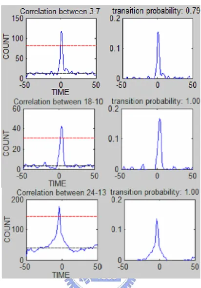
Figure 2.5: Cross–correlation functions and transition probability functions for selected pairs of entry/exit zones. Time is measured in seconds. Red line indicates the peak detection threshold, while the black line indicates the level of cross–correlation if the zones were uncorrelated [23].

dences is examined for a peak by thresholding based on the mean and standard deviation. Figure 2.5 shows examples of cross–correlation function and transition probability function for selected pairs of entry/exit zones.

Markis’ approach has been extended by Stauffer [24] and Tieu et al. [25] by providing a more rigorous definition of transition based on statistical significance. Stauffer tested the hypothesis that the correlation between exit and entry events that may or may not contain valid object transitions is similar to the expected correlation when there are no valid transitions. Tieu et al. also presented that the method of [23] suffers from the assumption of unimodal transition distribution,

Figure 2.6: Transition distributions obtained using correlation with different time windows all fail to match the simulated multi–modal distribution (dashed plot).In addition, there is no clear maximum peak indicating statistical dependence [25].

as shown in Figure 2.6. Unlike using cross–correlation in [23], their approaches used information–theoretic mutual information or entropy to compute statistical dependence between observations across cameras.

However, most of the features or models used in the above methods are in-sufficient in real life scenario for traffic flow surveillance. For example, in the wide–area surveillance, the appearance model may become invalid because the observation may occupy only a few pixels or looks very different from different viewing angles of cameras ,or under sudden lighting changes. Likewise, for ve-hicles in the real life traffic which might contain complicated behavior patterns such as car–following and queuing, the aforementioned object motion won’t be able to provide accurate descriptions. Moreover, due to the dynamic changes of real life traffic, the transition–time distribution may not be correctly found by cross–correlation or by maximizing the dependence between observations in two cameras.

2.2

Markov Chain Monte Carlo

dimensional spaces. As a result, it has been widely used in machine learning, physics, chemistry, biology statistics, and computer science. MCMC can be re-garded as a strategy for sampling from some complex distributions of interest. It is named after the fact that the next sample is randomly generate from the previ-ous sample by following a Markov chain mechanism, under which the transition probabilities between sample values are only a function of the most recent sample values. This mechanism can facilitate the chain to spend more time in more im-portant regions [26]. In the literature, different algorithms of MCMC have already been well developed. We will introduce two commonly used ones in this section.

2.2.1 The Metropolis–Hastings algorithm

One original motivation for applying MCMC comes from the attempt to handle the situations when we cannot directly draw samples from some complex proba-bility distributions. Metropolis–Hastings (MH) algorithm provides a general ap-proach for obtaining a sequence of random samples from those distributions. The sequence can then be used to approximate the distribution (i.e., to generate a his-togram). This algorithm is the most popular MCMC method [27, 28]. Many practical MCMC algorithms can be interpreted as special cases or extensions of this algorithm [29].

Suppose our goal is to draw samples from a probability distribution p(x), MH algorithm creates a Markov chain for sampling a candidate value x∗given the cur-rent value x according to a proposal distribution q(x∗|x). This new candidate is ac-cepted with acceptance probability A(x, x∗) = min{1, [p(x)q(x∗|x)]−1p(x∗)q(x|x∗)}; otherwise, the current value of x is retained. The pseudo–code of MH algorithm is listed in Figure 2.7.

Figure 2.7: Metropolis–Hastings algorithm.

The main idea of MH algorithm is to simulate sampling from the target dis-tribution p(x) by sampling from another easy–to–sample proposal disdis-tribution q(x∗|x). Hence, the more q(x∗|x) matches the shape of p(x), the better MH al-gorithm works. Besides, the term [p(x)q(x∗|x)]−1p(x∗)q(x|x∗) in the acceptance probability give us a measure about how much the Markov chain would like to move toward the candidate value x∗.

As shown in Figure 2.8, the authors in [29] give an example of running the MH algorithm based on a Gaussian proposal distribution q(x∗|x(i)_{) = N (x}(i)_{, 100)}

and a bimodal target distribution p(x) ∝ 0.3exp(−0.2x2)+0.7exp(−0.2(x−10)2) for 5000 iterations. As expected, the histogram of the samples approximates the target distribution.

2.2.2 The Gibbs sampler

Gibbs sampler [30], is a special case of the Metropolis–Hastings algorithm [26]. It is an algorithm to generate a sequence of samples from the joint probability

Figure 2.8: Target distribution and histogram of the MCMC samples at different iteration points [29].

one only considers univariate conditional distributions — the distribution when all of the random variables but one are kept fixed. Hence, this method is applicable when the joint distribution is not known explicitly but the univariate conditional distribution of each random variable is known.

Suppose we have an n–dimensional vector x and the expression for the full univariate conditional distribution p(xj|x−j) = p(xj|x1, . . . , xj−1, xj+1, . . . , xn).

By taking the following proposal distribution for j = 1, . . . , n

q(x∗|x(i)) =      p(x∗_j|x(i)_−j) If x∗_−j = x(i)_−j 0 Otherwise. (2.1)

Figure 2.9: Gibbs sampler.

The corresponding acceptance probability is: A(x(i), x∗) = min{1, p(x

∗_)q(x(i)_|x∗₎ p(x(i)_)q(x∗_|x(i)₎} (2.2) = min{1, p(x ∗_)p(x(i) j |x (i) −j) p(x(i)_)p(x∗ j|x∗−j) } = min{1, p(x ∗ −j) p(x(i)_−j) } = 1

Hence, the acceptance probability for each new candidate random value x∗is one. In other words, each new proposal sample is always accepted. The pseudo– code of Gibbs sampling is presented in Figure 2.9.

2.3

Expectation–Maximization

The Expectation Maximization algorithm (Hartley, 1958 [31]; Dempster et al., 1977 [32]; McLachlan and Krishnan, 1997 [33]) performs maximum likelihood

an expectation (E) step, which finds the distribution of the unobserved variables, given the known values for the observed variables and the current estimate of the parameters; and a maximization (M) step, which computes the parameters which maximize the expected likelihood found in the E step, under the assumption that the distribution found in E step is correct. These parameters are again used to determine the distribution of the unobserved variables in the next E step [34]. To understand the EM algorithm, we give a simple description of EM in the follow-ing.

Suppose that we have observed the value of some random variable, Z, but not the value of another latent variable, Y . The joint probability for these two variables is parameterized using θ, as P (y, z|θ). We want to find the maximum likelihood estimate for the parameter θ of a model for Y and Z, but this prob-lem cannot be easily solved directly. Alternatively, the corresponding probprob-lem in which Y is also known would be more tractable.

The basic idea of this problem is to maximize the log likelihood of the pa-rameter θ, given the data z, by marginalizing over the latent variable Y :

θ∗ = arg max θ log X Y P (y, z|θ) (2.3) = arg max θ log P (z|θ) = arg max θ L(θ).

This gives the intuition behind the EM algorithm: alternate between esti-mating the unknowns θ and estiesti-mating the hidden variable Y . The EM algorithm starts with some initial guess at the maximum likelihood parameters, θ(0), and then proceeds to iteratively generate successive estimates, θ(1), θ(2), . . . by repeatedly applying the following two steps, for t = 1, 2, . . .

– E Step: Compute a distribution ˜P(t) over the range of Y such that ˜

P(t)(y) = P (y|z, θ(t−1)).

– M step: Set θ(t) to the θ that maximizes E_P˜(t)[log P (y, z|θ)].

Here E_P˜[· ] denotes the expectation with respect to the distribution ˜P over the

range of Y [35]. As shown by Dempster, et al. [32], EM algorithm has the prop-erty of increasing the likelihood L(θ), or leave it unchanged, at each step. In fact, although an EM iteration does not decrease the observed data likelihood func-tion, it is not guaranteed to converge to a maximum likelihood estimate. For most models, the algorithm may converge to a local maximum of L(θ). Actually, we may also view EM algorithm as two alternating maximization steps for the same function F ( ˜P , θ) which is defined as follows:

F ( ˜P , θ) = E_P˜[log P (y, z|θ)] + H( ˜P ), (2.4)

where H( ˜P ) = −E_P˜[log ˜P (y)] is the entropy of the distribution ˜P . Hence, an

iteration of EM algorithm can be expressed in terms of the function F as follows: – E Step: Set ˜P(t) to the ˜P that maximizes F ( ˜P , θ(t−1)).

– M step: Set θ(t) to the θ that maximizes F ( ˜P(t), θ).

Once the EM iterations have been expressed in this form, it is clear to tell that the algorithm will eventually converge to the value ˜P∗ and θ∗ that locally maximize F ( ˜P , θ) [35].

3 Proposed Method

In this chapter, we present an algorithm to infer the traffic state between non– overlapping FOVs by modeling the traffic flow with a transition–time distribution which may change dynamically. We first introduce the targets selected for the analysis of traffic status in our system. By utilizing the specific motion pattern of the targets of interest, we can reduce the complexity of traffic flow analysis and improve the system performance. Then we will describe the traffic flow model of our system in Section 3.2. In Section 3.3, the problem formulation and our algorithm are presented. In Figure 3.1, we show the flowchart of the proposed system.

We have conducted some experiments based on a real life traffic environ-ment. Two cameras are installed to monitor two separate regions, which are linked by a road with some intersections in–between. More detailed description of the setting of our experimental environment and setting in the next chapter.

3.1

Selected Target

In order to monitor the traffic state between two non–overlapping FOVs linked by a road, we need to observe and analyze objects(cars) moving between the two FOVs. In general, however, since there may be intersections along the road, vehi-cles may leave or enter the road in–between. This circumstance will complicate the whole problem since we may have to identify the objects that leave halfway and ignore them in the traffic analysis. Accordingly, to alleviate the potential difficulty of analysis incurred by this case, we prefer to infer the traffic state be-tween non–overlapping FOVs by choosing the vehicles are more likely to have

Figure 3.1: The block diagram of the proposed system.

fixed route (e.g., bus) across FOVs as our main targets. Although we still cannot guarantee that all the buses seen in one FOV will definitely show up in another, this target selection can indeed improve the accuracy of our analysis. By selecting buses in the traffic videos obtained from two FOVs, we record the entry/exit times of all the buses in the regions of interest. A result of the target selection is shown in Figure 3.2.

3.2

Traffic Flow Model

From a microscopic point of view, every vehicle has its own behavior pattern, which is affected by individual driver. However, if observed from a macroscopic point of view, one may find that most vehicles typically follow a global trend that is affected by the interactions among vehicles such as car–following and queuing.

Figure 3.2: A result of target selection. We choose buses as our targets and record the exit time ({xm}m=1∼M)

and entry time ({yn}n=1∼N) of them.

tion model. Here we use the Gaussian mixture model (GMM) to approximate this distribution because this model is general and can well approximate a lot of con-tinuous functions under normal conditions. Some examples of distributions in the real life traffic are shown in Figure 3.3, in which we can see that the distributions can be well modeled by GMM. With the assumption of GMM model, our objec-tive is to derive the parameters of this global transition time model to describe the traffic state. Moreover, since traffic flow state may dynamically change over time, we divide the timeline into many overlapped time–windows to analyze the transition time distributions at different times of the day, as shown in Figure 3.4.

Figure 3.3: Some examples of distributions in the real life traffic.

Figure 3.4: Division the timeline of the day into overlapped time–windows.

3.3

Problem Formulation

Before discussing how to determine the GMM parameters, we first consider two problem from two opposite viewing angles in the following paragraphs. First, suppose that we have the prior knowledge of the global transition–time distri-bution, we may infer the rough correspondence among buses. That is, we can approximately determine how the buses in two FOVs match one another. On the other hand, if we know how the buses in two FOVs match one another and thus the transition time of each correspondence, the global transition time distribution can be derived. Hence, in our system, we exploit this physical dependence be-tween the correspondences of buses and the global transition–time distribution,

independent of each other. Without loss of generality, we only discuss the traffic problems in a single side.

To determine the model parameters and to further infer the traffic state within a time window, we formulate the problem as an optimization process expressed as follows:

Θ∗ = arg max

Θ p(Θ|Z), (3.1)

where Z = ({xm}M, {yn}N) represents the combination of observations,

includ-ing the exit time set (x1, x2, . . . , xm, . . . , xM) and the entry time set (y1, y2, . . . , yn,

. . . , yN) of all the buses in two non–overlapping FOVs, as shown in Figure 3.2.

However, it is difficult to build the probability model P (Θ|Z) in Equation 3.1, owing to the lack of physical connection between Θ and Z. To compensate the physical gap between parameters Θ and our observations Z, we introduce the cor-respondences between the exit time {xm}M and entry time {yn}N as an unknown

random variable C = {cm(xm) = yn}M, where cm(.) indicates the entry time yn

that an exit time xm will correspond to. Therefore, if a bus leaves one FOV at

xm, travels through the road, and then enters another FOV at yn, we can express

this correspondence by {xm, cm(xm) = yn}. The transition time of this

corre-spondence is tm = cm(xm) − xm. Figure 3.5 shows the schematic diagram of

xm, yn, cm(.), and tm. By collecting all the transition times of each

correspon-dence into a data set T = {tm}M, we may estimate the model parameters Θ.

The problem of the above formulation is that we do not have the measure-ment of C and we cannot derive the Θ directly. Hence, we treat the correspon-dence C as a latent variable and reformulate Equation 3.1 as Equatiion 3.2 by

Figure 3.5: The schematic diagram of xm, yn, cm(.), and tm.

marginalizing out every possible correspondence C. Θ∗ = arg max

Θ

X

C

p(Θ, C|Z). (3.2)

Although a direct approach to solving this optimization problem is generally intractable, the Expectation Maximization algorithm provides a mean to do the maximization by iteratively calculating the following two steps:

1. E Step: Calculate the expected log likelihood function Q(Θ): Q(Θ) =X

C

log(p(Z, C|Θ))p(C|Z, Θ(old)). (3.3)

where the expectation is taken with respect to the posterior distribution p(C|Z, Θ(old)) over all possible correspondences C, given the data Z and the Θ(old) at the previous time step.

2. M step: Find the Maximum Likelihood estimate Θ(new) by maximizing Q(Θ): Θ(new) = arg max

Figure 3.6: Gibbs sampler in the proposed method.

Markov chain Monte Carlo (MCMC) to sample from the posterior probability distribution p(C|Z, Θ(old)) and replace the expectation in the E step over all pos-sible correspondences with MCMC samples. More formally, this can be justi-fied in the context of a Monte Carlo EM or MCEM. The sampling method we use here is the Gibbs sampling. In our setting, it is prefered that the entry/exit times are having one–to–one correspondences, but still allow the possibility that one entry time could be matched with more than one exit times. Therefore, p(cj|c (r+1) 1 , . . . , c (r+1) j−1 , c (r) j+1, . . . , c (r)

M, Θ), the conditional probability of cj given

the other correspondences {cm}M 6=j and global transition time distribution Θ, will

be proportional to the likelihood of transition time tj = cj(xj) − xj determined

by Θ, while the conditional probability may decrease if the exit time yn = cj(xj)

has been matched with others (see the algorithm in Figure 3.6). A simple example of the process in Gibbs sampling is shown in Figure 3.7. By performing sampling R times, it will generate a sequence of C. Since we expect that the correct C will have a much higher likelihood than others, we will choose the best sampling result to enter the M step in the EM algorithm.

(a)

(b)

Figure 3.7: A simple example of the Gibbs sampling. (a) In the beginning, for sampling c1, there are four

can-didates: c1(x1) = y1, c1(x1) = y2, c1(x1) = y3, c1(x1) = y4 and therefore four possible transition times:

t1−1, t1−2, t1−3, t1−4. For every transition time we can measure its likelihood to the distribution Θ. The Gibbs

sampling will sample c1according to the probability proportional to these likelihoods. Here we assume the Gibbs

de-With the correspondences C = {cm}M from the Gibbs sampling, we can

calculate all the transition times {tm = cm(xm) − xm}M of buses traveling across

two non–overlapping FOVs. In the M step, from {tm}M, we will derive the

pa-rameters Θ of the global transition time distribution. Assume we use a GMM with K Gaussians to approximate the global transition time distribution, then the dis-tribution Θ will be parameterized by the weight wj, the mean µj, and the variance

σ_j2of the jth Gaussian, with j = 1, . . . , K. To estimate these parameters given the transition times {tm}M, we can use a standard EM algorithm designed for GMM

that is based on the following iteration formulae: w_j(r+1) = 1 n M X m=1 P (j|tm) (3.5) µ(r+1)_j = M P m=1 P (j|tm)tm M P m=1 P (j|tm) (3.6) σ2(r+1)_j = M P m=1 P (j|tm)(tm − µ (t+1) j ) 2 M P m=1 P (j|tm) (3.7) where P (j|tm) = w(r)_j p(tm|j; µ (r) j , σ (r) j ) K P k=1 w_k(r)p(tm|k; µ (r) k , σ (r) k ) . (3.8)

A demonstration of the M step is shown in Figure 3.8.

The global transition–time distribution parameterized by {wj, µj, σj2}K

dis-covered in the M step will be propagated into the E step of the next EM iteration. After a few iterations, the EM algorithm will converge to a maxima of p(Θ|Z). The proposed EM algorithm for traffic state monitoring within a time–window is shown in Figure 3.9.

Figure 3.8: A demonstration of the M step. With the transition times calculated from the correspondence from the Gibbs sampling, we use the EM algorithm to estimate the parameters of the GMM in order to model the transition time distribution.

Figure 3.10: Initialization of the EM algorithm for the first time–window. We start the EM iteration by initial-izing the global transition–time distribution Θ with the Gaussian mixture model of K equal weighting, broadly separated, and wide–bandwidth Gaussians. We assume this initialization of GMM can cover most regions of the transition time.

3.4

Initialization

In this paper, we divide the timeline into several overlapped time–windows to han-dle the dynamic changes of the traffic flow, as shown in Figure 3.4, and apply the proposed EM algorithm to every time–window. An important step for performing the proposed EM algorithm in each time–window is the initial setting. For the first time–window, we start the EM iteration by initializing the global transition–time distribution Θ with the Gaussian mixture model of K equal weighting, broadly separated, and wide–bandwidth Gaussians, as shown in Figure 3.10. We assume this initialization of GMM can cover most regions of the transition time.

On the other hand, for the initial setting of the subsequent time–windows, since they are partially overlapped with the previous ones, we would like to prop-agate some information from the previous window into the current window as the initial condition. Hence, we have two choices for the initialization – propagating either the parameters of the Gaussian mixture model or the correspondences from

Figure 3.11: A possible situation for the current time–window and the previous one — the transition–time distri-bution of the current time–window is more widespread then it of the previous window. The increased range of the transition–time is caused from the data in the non–overlapped subsection which is new to the last time window (noted with the blue bounding–box), and the GMM of the previous time–window only has the information of the overlapped subsection in current time–window (noted with the purple bounding–box).

the previous window. Consider a possible situation wherein the transition–time distribution of the current time–window is more widespread than that of the pre-vious one, as shown in Figure 3.11. The increased range of the transition time due to the new data (marked with the blue bounding–box) is not covered by the GMM of the previous time–window (marked with the purple bounding–box). As a result, if we start the EM iterations by initializing the parameters of GMM which are propagated from the previous time window, the algorithm may only cover the partial range of the transition time and lead to incorrect result.

Therefore, for the EM initialization of the subsequent time–windows, in ad-dition to propagate the correspondences of the overlapped subsections from the

Figure 3.12: Initialization of the EM for the following time–windows. We propagate the correspondences of the overlapped subsection from the previous window into the current window, and randomly assign the correspon-dences of the new data in the non–overlapped subsection.

dow, we randomly assign the correspondences within this period. That is, we start the EM iterations by initializing the correspondences C which consist of both the propagated and the randomly assigned correspondences, as shown in Figure 3.12. This method for initialization helps the algorithm to maintain some information from the previous time–window, while still have the ability to extract useful infor-mation from the new data.

4 Experiment and Results

Out experimental environment is shown in Figure 4.1. We mounted two cameras at the Mackay Memorial Hospital and the overpass in front of National Tsing Hua University. In Figure 4.1, we can see that FOVs of these two cameras are non-overlapped and these two scenes are linked by Kuang Fu Road (indicated by the red line). Besides, there are three intersections and some bus stops along the road between these two FOVs. This makes the traffic situations more complicated. The traffic videos were taken from about 9:45 in the morning till 19:00 in the afternoon. We divide the time–line into 34 overlapped time–windows. The length of each time–window is 60 minutes, with 45 minutes overlapped with the previous window, as shown in Figure 4.2

We first check the traffic videos and manually select frames that contain buses. All the entry/exit times of buses are recorded. Then we apply the proposed EM algorithm for each time–window. Here we use a Gaussian mixture model with 3 Gaussians to model the transition–time distribution. For the first time– window, the parameters of the GMM are initialized with µ = {50, 150, 250}, σ2 = {200, 200, 200} and w = {0.33, 0.33, 0.33}. Then the initialization for EM in all the other time–windows follows the method we described in Section 3.4. Figure 4.3, Figure 4.4, and Figure 4.5 show the computed transition–time distri-butions and the ground–truths in different time–windows. We can see that the distribution calculated by our algorithm is reasonably similar to the ground truth.

Here we also give some results by applying the method in [25] to our experi-mental data, as shown in Figure 4.6. We can see that the results are not as accurate

Figure 4.1: The experimental environment: monitor the traffic between two non–overlapping FOVs at Mackay Memorial Hospital and the NTHU overpass.

Figure 4.2: We divide the timeline into 34 overlapped time–windows. The length of each time–window is 60 minutes, with 45 minutes overlapped with the previous window.

(a) (b) (c)

(d) (e) (f)

(g) (h) (i)

(j) (k) (l)

Figure 4.3: The transition–time distribution from time–window # 01 to time–window # 12.

(a) Time–window 09 : 45 ∼ 10 : 45. (b) Time–window 10 : 00 ∼ 11 : 00. (c) Time–window 10 : 15 ∼ 11 : 15. (d) Time–window 10 : 30 ∼ 11 : 30. (e) Time–window 10 : 45 ∼ 11 : 45. (f) Time–window 11 : 00 ∼ 12 : 00. (g) Time–window 11 : 15 ∼ 12 : 15. (h) Time–window 11 : 30 ∼ 12 : 30. (i) Time–window 11 : 45 ∼ 12 : 45. (j) Time–window 12 : 00 ∼ 13 : 00. (k) Time–window 12 : 15 ∼ 13 : 15. (l) Time–window 12 : 30 ∼ 13 : 30.

(a) (b) (c)

(d) (e) (f)

(g) (h) (i)

(j) (k) (l)

Figure 4.4: The transition–time distribution from time–window # 13 to time–window # 24.

(a) Time–window 12 : 45 ∼ 13 : 45. (b) Time–window 13 : 00 ∼ 14 : 00. (c) Time–window 13 : 15 ∼ 14 : 15. (d) Time–window 13 : 30 ∼ 14 : 30. (e) Time–window 13 : 45 ∼ 14 : 45. (f) Time–window 14 : 00 ∼ 15 : 00. (g) Time–window 14 : 15 ∼ 15 : 15. (h) Time–window 14 : 30 ∼ 15 : 30. (i) Time–window 14 : 45 ∼ 15 : 45. (j) Time–window 15 : 00 ∼ 16 : 00. (k) Time–window 15 : 15 ∼ 16 : 15. (l) Time–window 15 : 30 ∼ 16 : 30. (x–axis: transition time; y–axis: milli–probability).

(a) (b) (c)

(d) (e) (f)

(g) (h) (i)

(j)

Figure 4.5: The transition–time distribution from time–window # 25 to time–window # 34.

(a) Time–window 15 : 45 ∼ 16 : 45. (b) Time–window 16 : 00 ∼ 17 : 00. (c) Time–window 16 : 15 ∼ 17 : 15. (d) Time–window 16 : 30 ∼ 17 : 30. (e) Time–window 16 : 45 ∼ 17 : 45. (f) Time–window 17 : 00 ∼ 18 : 00. (g) Time–window 17 : 15 ∼ 18 : 15. (h) Time–window 17 : 30 ∼ 18 : 30. (i) Time–window 17 : 45 ∼ 18 : 45. (j) Time–window 18 : 00 ∼ 19 : 00.

(a) (b) (c)

Figure 4.6: Some results from applying the method in [25] to our experimental data. (a) Time–window 12 : 00 ∼ 13 : 00. (b) Time–window 12 : 15 ∼ 13 : 15. (c) Time–window 17 : 00 ∼ 18 : 00.

characteristics of the real life traffic while the method in [25] only depends on the weaker minimum entropy assumption about the transition time distribution. For example, in Figure 4.6(c), the distribution of the ground truth has a wider range and thus has a larger entropy value than that of the distribution found by the algorithm in [25].

To infer the traffic flow state, we can first use the average transition time of the last 15–minute observation within each time–window as a statistic to represent the state. As shown in Figure 4.7, the chart of the traffic–flow state may give us the direct message about how the traffic dynamically changes over time. For in-stance, we may probably guess that the increase of the average transition time at about 12:00 is due to the lunch–time traffic, which is always a rush hour. More-over, we could also express the traffic flow state by classifying the traffic changes as “stable”, “increasing”, and “decreasing,” as shown in Figure 4.8. This figure indicates how the traffic changes with respect to the previous stage. This kind of description is much more user–friendly.

In addition to the aforementioned setting of the time–line division and the ini-tialization method, here we provide some examples of different settings to support

that our setting is reasonable. In the first example of different settings, we divide the time–line into 60–minute time–windows with 30 minutes overlapped with the previous window. For the EM initialization of the following time–windows, we propagate the parameters of GMM from the previous window. Figure 4.9 shows the transition–time distributions of some time–windows. We can see that the com-puted transition–time distributions cannot adapt quickly enough to the changes of the ground truth. One reason for this phenomenon is due to the problem of initial-ization we presented in Figure 3.11. Moreover, since the information propagated from the previous window only dominates 50% of the data in the processing win-dow, the degree of change for the transition–time distribution might be too big to be tracked by the algorithm. Then, in the second example of different setting, we use the same time–windows as in the first example; and for the EM initialization of the following time–windows, we follows the method described in Section 3.4. Figure 4.10 shows the transition–time distributions of the time–windows which are the same as those in Figure 4.9. We can see that even there are some im-provement in Figures 4.9(b), 4.9(d), and 4.9(e), the problem of miss–tracking still exists, as shown in Figure 4.9(c). Hence, in our experiment, we choose to di-vide the timeline into time–windows with much more overlaps with the previous time-window.

Figure 4.7: Traffic flow state expressed by the average transition time of the last 15–minute observation within each time–window. The red line is computed by our proposed method; The blue line is from the ground truth.

Figure 4.8: Express the traffic flow state by classifying the traffic changes as “stable”, “increasing”, and “decreas-ing.” (Green color: stable traffic; Red color: increasing traffic flow; Blue color: decreasing traffic flow).

(a) (b) (c)

(d) (e) (f)

Figure 4.9: Some transition–time distributions from the first example of different setting. Each time–windows is 60 minutes long including 30 minutes overlapped with the previous window. The EM initialization of the following time–windows is with the parameters of GMM propagated from the previous window.

(a) Time–window 10 : 45 ∼ 11 : 45. (b) Time–window 11 : 15 ∼ 12 : 15. (c) Time–window 11 : 45 ∼ 12 : 45. (d) Time–window 12 : 15 ∼ 13 : 15. (e) Time–window 12 : 45 ∼ 13 : 45. (f) Time–window 13 : 15 ∼ 14 : 15. (x–axis: transition time; y–axis: milli–probability).

(a) (b) (c)

(d) (e) (f)

Figure 4.10: Some transition–time distributions from the second example of different setting. Each time–windows is 60 minutes long including 30 minutes overlapped with the previous window. The EM initialization of the following time–windows follows the method described in Section 3.4.

(a) Time–window 10 : 45 ∼ 11 : 45. (b) Time–window 11 : 15 ∼ 12 : 15. (c) Time–window 11 : 45 ∼ 12 : 45. (d) Time–window 12 : 15 ∼ 13 : 15. (e) Time–window 12 : 45 ∼ 13 : 45. (f) Time–window 13 : 15 ∼ 14 : 15. (x–axis: transition time; y–axis: milli–probability).

5 Conclusion

We propose an efficient method to probabilistically model the dynamic traffic flow between non–overlapping FOVs. Unlike previous works, our approach does not attempt to directly build the object correspondence across non–overlapping cam-eras. Instead, we model object correspondence and the parameters estimation of the transition time model as a unified problem. By building the physical con-nection between the transition time model and the object correspondence, the proposed EM–based framework can iteratively determine the optimal object cor-respondence and the model parameters. In addition, by dividing the time–line into many overlapped time–windows, our method can sequentially infer the time– varying traffic flow and recognize the dynamic changes of the traffic status over time. Moreover, our system is efficient and may provide a new thinking to well utilize the existing surveillance cameras for wide–area traffic monitoring. The ex-periments have shown that our approach performs well in a complicated traffic environment in real life.

Bibliography

[1] F.A. Haight. Mathematical theories of traffic flow. Academic Press, 1963. [2] D.L. Gerlough and M.J. Huber. Traffic flow theory. Transportation Research

Board, pages 199–201, 1975.

[3] A.D. May. Traffic flow fundamentals. Prentice Hall, 1990.

[4] N.H. Gartner, C.J. Messer, and A. Rathi. Special Report 165: Revised Mono-graph on Traffic Flow Theory. Transportation Research Board, Washington, DC, 1997.

[5] F. Viti. The dynamics and the uncertainty of delays at signals. PhD thesis, Delft University of Technology, 2006.

[6] H.J. van Zuylen and F. Viti. Delay at Controlled Intersections: The Old Theory Revised. In IEEE Intelligent Transportation Systems Conference, pages 68–73, 2006.

[7] D.J. Dailey, S.D. Maclean, F.W. Cathey, and Z.R. Wall. Transit vehicle arrival prediction: Algorithm and large–scale implementation. Transportation Re-search Record: Journal of the Transportation ReRe-search Board, 1771(-1):46– 51, 2001.

[8] D.J. Dailey, Z.R. Wall, S.D. Maclean, and F.W. Cathey. An algorithm and implementation to predict the arrival of transit vehicles. IEEE Intelligent Transportation Systems, pages 161–166, 2000.

[9] F.W. Cathey and D.J. Dailey. A prescription for transit arrival/departure pre-diction using automatic vehicle location data. Transportation Research Part C, 11(3-4):241–264, 2003.

[10] Z.R. Wall and D.J. Dailey. An algorithm for predicting the arrival time of mass transit vehicles using automatic vehicle location data. University of Washington, 1998.

[11] I. Steven, Y. Ding, and C. Wei. Dynamic bus arrival time prediction with artificial neural networks. Journal of Transportation Engineering, 128:429, 2002.

[12] Y. Bin, Y. Zhongzhen, and Y. Baozhen. Bus arrival time prediction us-ing support vector machines. Journal of Intelligent Transportation Systems, 10(4):151–158, 2006.

[13] B. Fishbain, I. Ideses, D. Mahalel, and L. Yaroslavsky. Real–time vision– based traffic flow measurements and incident detection. In Proceedings of SPIE, volume 7244, page 72440I, 2009.

[14] V. Kastrinaki, M. Zervakis, and K. Kalaitzakis. A survey of video processing techniques for traffic applications. Image and Vision Computing, 21(4):359– 381, 2003.

[15] D. Beymer, P. McLauchlan, B. Coifman, and J. Malik. A real–time computer vision system for measuring traffic parameters. In IEEE Computer Society

Conference on Computer Vision and Pattern Recognition, pages 495–501, 1997.

[16] B. Coifman, D. Beymer, P. McLauchlan, and J. Malik. A real–time computer vision system for vehicle tracking and traffic surveillance. Transportation Research Part C, 6(4):271–288, 1998.

[17] Z. Kim and J. Malik. Fast vehicle detection with probabilistic feature group-ing and its application to vehicle trackgroup-ing. In Proc. 9th IEEE International Conference on Computer Vision, Nice, France, volume 1, pages 524–531, 2003.

[18] O. Javed, K. Shafique, Z. Rasheed, and M. Shah. Modeling inter– camera space–time and appearance relationships for tracking across non– overlapping views. Computer Vision and Image Understanding, 109(2):146– 162, 2008.

[19] O. Javed, Z. Rasheed, K. Shafique, and M. Shah. Tracking across multiple cameras with disjoint views. In Ninth IEEE International Conference on Computer Vision, pages 952–957, 2003.

[20] B. Song and A.K. Roy-Chowdhury. Stochastic adaptive tracking in a camera network. In IEEE 11th International Conference on Computer Vision, pages 1–8, 2007.

[21] A. Rahimi, B. Dunagan, and T. Darrell. Simultaneous calibration and track-ing with a network of non–overlapptrack-ing sensors. In IEEE Computer Society Conference on Computer Vision and Pattern Recognition, volume 1, pages

[22] Y. Sheikh, X. Li, and M. Shah. Trajectory association across non– overlapping moving cameras in planar scenes. In IEEE Computer Society Conference on Computer Vision and Pattern Recognition, pages 1–7, 2007. [23] D. Makris, T. Ellis, and J. Black. Bridging the gaps between cameras. In

IEEE Computer Society Conference on Computer Vision and Pattern Recog-nition, volume 2, 2004.

[24] C. Stauffer. Learning to track objects through unobserved regions. In IEEE Computer Society Workshop on Motion and Video Computing, volume 2, 2005.

[25] K. Tieu, G. Dalley, and W.E.L. Grimson. Inference of non–overlapping cam-era network topology by measuring statistical dependence. In Tenth IEEE International Conference on Computer Vision, volume 2, 2005.

[26] W.R. Gilks, S. Richardson, and D.J. Spiegelhalter. Markov chain Monte Carlo in practice. Chapman & Hall/CRC, 1996.

[27] W.K. Hastings. Monte Carlo sampling methods using Markov chains and their applications. Biometrika, 57(1):97–109, 1970.

[28] N. Metropolis, A. Rosenbluth, M. Rosenbluth, A. Teller, and E. Teller. Equa-tions of state calculaEqua-tions by fast computational machine. Journal of Chemi-cal Physics, 21(6):1087–1091, 1953.

[29] C. Andrieu, N. De Freitas, A. Doucet, and M.I. Jordan. An introduction to MCMC for machine learning. Machine learning, 50(1-2):5–43, 2003.

[30] S. Geman and D. Geman. Stochastic relaxation, Gibbs distributions, and the Bayesian restoration of images. In IEEE Transactions on Pattern Analysis and Machine Intelligence, 1984.

[31] H.O. Hartley. Maximum likelihood estimation from incomplete data. Bio-metrics, pages 174–194, 1958.

[32] A.P. Dempster, N.M. Laird, D.B. Rubin, et al. Maximum likelihood from in-complete data via the EM algorithm. Journal of the Royal Statistical Society. Series B (Methodological), 39(1):1–38, 1977.

[33] G.J. McLachlan, T. Krishnan, and W. InterScience. The EM algorithm and extensions. Wiley New York, 1997.

[34] F. Dellaert. The expectation maximization algorithm. Georgia Institute of Technology, Technical Report Number GIT-GVU-02-20, 2002.

[35] R.M. Neal and G.E. Hinton. A view of the EM algorithm that justifies incre-mental, sparse, and other variants. Learning in graphical models, 89:355– 368, 1998.