A Conservative Scheme for Solving Coupled Surface-Bulk Convection-Diffusion Equations with an Application to Interfacial Flows with Soluble Surfactant

A conservative scheme for solving coupled

surface-bulk convection-diffusion equations with an

application to interfacial flows with soluble

surfactant

Kuan-Yu Chen∗ _{Ming-Chih Lai}†

Abstract

Many physical problems arising in biological or material sciences in-volve solving partial differential equations in deformable interfaces or complex domains. For instance, the surfactant (an amphiphilic molec-ular) which usually favors the presence in the fluid interface may couple with the surfactant soluble in one of bulk domains through adsorption and desorption processes. Thus, it is important to accurately solve cou-pled surface-bulk convection-diffusion equations especially when the interface is moving. In this paper, we first rewrite the original bulk concentration equation in soluble region into a whole computational domain via the usage of the indicator function so that the concentration flux across the interface due to adsorption and desorption processes can be termed as a singular source in the equation. Based on the immersed boundary formulation, we develop a new conservative scheme for solv-ing the coupled surface-bulk concentration equations which the total surfactant mass is conserved exactly in discrete sense. A series of nu-merical tests has been conducted to validate the present scheme. As an application, we extend our previous work ”M.-C. Lai, Y.-H. Tseng and H. Huang, An immersed boundary method for interfacial flows with insoluble surfactant, Journal of Computational Physics, 227 (2008) 7279-7293” to the soluble case. The effect of solubility of surfactant on drop deformation in a shear flow is investigated in detail.

Keywords: a conservative scheme; interfacial flow; soluble surfac-tant; adsorption-desorption process; immersed boundary method

∗_{Department of Applied Mathematics, National Chiao Tung University, 1001, Ta Hsueh}

Road, Hsinchu 30010, Taiwan. E-mail: [email protected]

†_{Corresponding author. Center of Mathematical Modeling and Scientific Computing}

& Department of Applied Mathematics, National Chiao Tung University, 1001, Ta Hsueh Road, Hsinchu 30010, Taiwan. E-mail: [email protected]

1

Introduction

Many problems in biological, physical and material sciences involve solv-ing partial differential equations in complex domains or deformable inter-faces. In particular, the underlying material quantities in the bulk domain may couple with the one in the interface through adsorption and desorption process. Meanwhile, the concentration of surface quantities might change the physical behavior of the interface through the modifications of inter-facial forces. For instance, surfactant molecules typically consisting of a hydrophilic head and a hydrophobic tail may adsorb and desorb between bulk fluids and the interface so that the interfacial tension can be reduced. Meanwhile, this non-uniform distribution of surfactant molecules produce extra force (Marangoni force) along the tangential direction to affect the dynamics. In practice, the surfactant may be soluble only to some portion of bulk domain enclosed by the interface where the interface and the soluble region are evolving simultaneously. In order to simulate this problem, we have to introduce two surfactant concentrations in the system; namely, the surface concentration along the interface, and the volume concentration in the bulk region. Thus, one need to solve a coupled system of surface-bulk convection-diffusion equations [18, 30, 24].

Another example comes from cell biology applications where proteins inside the cell can diffuse and bind to the membrane whereas membrane-bound proteins can dissociate and diffuse to the inner cytoplasm [19]. To simulate this problem, one need to solve a coupled system of surface-volume reaction-diffusion equations. Many other examples in physical and biological systems that have the similar adsorption or desorption mechanisms in the dynamics can be found in the reference [24].

It is known that solving a coupled system of surface-bulk equations in complex domains or deformable interfaces numerically is quite challenging especially when the interface (or the interior boundary of domains) is mov-ing. Even in the case of only surface material (without bulk coupling), de-veloping numerical methods for convection-diffusion equations on an evolv-ing interface is still of major interest in scientific computevolv-ing community. These methods include surface element method [5, 6, 9, 10], level set method [2, 7, 27, 23, 17], and phase field method [22, 24, 11], just to name a few. Front tracking method is typically more accurate for one-dimensional inter-face (a curve in 2D space), but it can be more complicated to implement for two-dimensional surface especially the implementation involves surface mesh distortion or even topological changes. In [14], we have successfully developed a mass conservative scheme for convection-diffusion equation on

moving interface and applied to simulate the interfacial flows with insoluble surfactant [14, 15, 16]. A recent work of Khatri and Tornberg [13] used seg-ment projection method to represent the interface and solve the surfactant equation. More up-to-dated numerical methods for solving Navier-Stokes flows with insoluble surfactant can be found in [13] as well.

In this paper, we shall extend our previous work to soluble surfactant case. However, as a very first step, we need to develop a conservative scheme for solving coupled surface-bulk convection-diffusion equations. There are at least three major numerical issues from our point of view. (1) How to handle the adsorption and desorption between the interface and the bulk accurately? (2) How to maintain the total surfactant mass conserved dur-ing the evolution? (3) Since the surfactant might be soluble to only one of buck fluid, how to avoid the surfactant being present in other bulk regions via either convection or diffusion mechanism? Here, we formulate the cou-pled surface-bulk convection-diffusion equations in the immersed boundary framework so that the adsorption and desorption processes can be termed as a singular source in the bulk equation. Moreover, by using the indica-tor function, we can embed the bulk equation into the whole computational domain so that regular Eulerian finite difference scheme can be applied with-out handling the complicated moving irregular domain. We develop a new conservative scheme for solving the coupled bulk-surface concentration equa-tions which the total surfactant mass can be conserved exactly in discrete sense. By introducing the indicator function and solving the bulk equation in the whole computational domain, one can avoid evaluating the surfactant flux across the interface due to adsorption and desorption processes.

The present formulation is similar to other front tracking approaches such as in [30, 18] but differs from their numerical computations. For in-stance, in order to let the surfactant be depleted from only one bulk phase, some one-sided discretized delta functions were used in [30] which results the numerical integration of the discrete function does not yield the exact value of unity. The authors have tried different forms of one-sided delta func-tion and the mass error is within 1%. Here, we use the tradifunc-tional discrete delta function for the spreading and interpolating operators in the immersed boundary method so that the surfactant mass leaking error is much smaller compared with [30]. There are other numerical methods in literature for interfacial flows with soluble surfactant dynamics such as in [1, 4, 25, 29].

The rest of the paper is organized as follows. In Section 2, we present a coupled surface-bulk concentration model and discuss their conservation property. By employing the indicator function, we then embed the bulk equation into the whole computational domain. Based on our immersed

boundary formulation, we develop a conservative scheme for solving the coupled surface-bulk equations in Section 3. As an application, we apply the present scheme to solve Navier-Stokes flow with soluble surfactant in Section 4. In Section 5, a detailed numerical tests have been conducted to validate our present scheme and study the effect of soluble surfactant on drop deformation in a shear flow.

2

A coupled surface-bulk concentration model

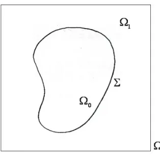
As in [24], we consider the same coupled bulk-surface material (or surfactant) concentration model in which the adsorption and desorption can be occurred on the moving deformable interface. Consider a domain Ω in R2 _{and there}

is an interface Σ, which is a simple closed curve immersed in Ω. The interior of the interface is Ω₀, and the exterior is Ω₁ so that Ω = Ω₀∪ Ω₁, see the illustration of these domains in Figure 1. The interface is represented by a Lagrangian form X(s, t), 0 ≤ s ≤ L_b, where s is the Lagrangian material coordinate attached to the interface which is not necessarily to be the arc-length parameter. The unit tangent vector of the interface can be written as τ = ∂X ∂s / ¯ ¯ ¯∂_∂sX ¯ ¯

¯; thus, the unit outward normal vector n pointing into Ω1 can be defined accordingly. In addition, the interface Σ is moving with

a given velocity field u = (u, v) in Ω; that is, ∂X(s, t)

∂t = U (s, t) = Z

Ω

u(x, t)δ2(x − X(s, t)) dx, (1) where δ2_{(x) = δ(x) δ(y) is the two-dimensional Dirac delta function. We}

use the above usual delta function formulation in the immersed boundary method [20] to represent the interpolation of the velocity field into the in-terface. Here we assume the velocity field is incompressible (∇ · u = 0) in Ω and no flow boundary condition (u · n1 = 0) is imposed on ∂Ω = ∂Ω1.

Notice that, in later section, the velocity field can be obtained by solving the Navier-Stokes equations.

It is assumed that the surfactant exists on the interface as a monolayer and is adsorbed from or desorbed into the bulk fluid in Ω₁; that is, the surfactant is soluble in the exterior bulk Ω1 but not in the interior one

Ω0. Therefore, we have to introduce two surfactant concentrations in the

system; namely, the surface concentration Γ along the interface Σ, and the volume concentration C in the bulk region Ω1. By taking the adsorption

Figure 1: Illustration of domains. concentration equation can be modified as

∂Γ

∂t + (∇s· u) Γ = 1 P es

∇2_sΓ + SaCs(1 − Γ) − SdΓ, (2)

where ∇s= (I −n⊗n)∇ and ∇2s= ∇s·∇sare the surface gradient and

sur-face Laplacian operators, respectively. The dimensionless number P es is the

surface Peclet number, Saand Sdare the absorption and desorption Stanton

number, respectively. Cs is the bulk surfactant concentration adjacent to

the interface which can be defined later. The above non-dimensionalization process can be found in [30, 18, 14]. Notice that, as in [14], the interface is tracked in Lagrangian manner and the surface concentration is defined at the material point, so the time derivative in Eq. (2) has the meaning of the material derivative naturally.

The dimensionless volume concentration in the exterior region Ω₁ [18, 24, 25] can be written as ∂C ∂t + u · ∇C = 1 P e∇ 2_{C (3)} 1 P e ∂C ∂n|Σ = SaCs(1 − Γ) − SdΓ ∂C ∂n1|∂Ω1 = 0, (4)

where P e is the Peclet number, n is the unit normal vector on Σ pointing into Ω1 and n1 is the unit outward normal to the boundary ∂Ω1 = ∂Ω.

Eqs. (2)-(4) describe the present coupled bulk-surface concentration equa-tions. Since the fluid is incompressible and no flow velocity boundary con-dition is imposed on ∂Ω1, one can conclude that the total surfactant mass

(the surfactant mass on the interface Σ and the mass in the bulk region Ω₁) must be conserved. The conservation property can be proved easily as follows.

By first taking the integration of Γ over the interface, then applying the time derivative and using Eq. (2), the rate of change of surfactant mass in the interface Σ can be written as

d dt Z Σ Γdl = Z Σ µ ∂Γ ∂t + (∇s· u) Γ ¶ dl = Z Σ µ 1 P es∇ 2 sΓ + SaCs(1 − Γ) − SdΓ ¶ dl = Z Σ (S_aC_s(1 − Γ) − S_dΓ)dl, (5) where dl = ¯ ¯ ¯∂_∂sX ¯ ¯

¯ ds is the arc-length element. The last equality is obtained by using the fact that Σ is a closed interface. Similarly, the rate of change of surfactant mass in the bulk region Ω1 can be obtained by taking the

integration of C over the region Ω1, applying the time derivative, and then

using Eq. (3) as d dt Z Ω1 Cdx = Z Ω1 DC Dt dx = Z Ω1 1 P e∇ 2_{Cdx =} Z ∂Ω1 1 P e ∂C ∂n1dl − Z Σ 1 P e ∂C ∂ndl = − Z Σ (SaCs(1 − Γ) − SdΓ)dl, (6)

where the last equality is obtained by using the boundary conditions of Eq. (4). One can immediately lead to the total surfactant mass conservation by summing Eq. (5) and Eq. (6) so we have

d dt µZ Σ Γdl + Z Ω1 Cdx ¶ = 0. (7)

In summary, to obtain the present surface-bulk concentration, one need to solve a coupled convection-diffusion PDE system on an evolving interface and in an evolving irregular domain.

2.1 An embedding bulk concentration equation in the whole domain

As mentioned before, solving the bulk concentration equation involves solv-ing a convection-diffusion equation in an evolvsolv-ing irregular domain. In order to describe the solution in the whole domain Ω = Ω0∪ Ω1, we introduce the

indicator function H defined as H(x, t) = 1 − Z Ω0 δ2(x − ˜x) d˜x = ½ 1 if x ∈ Ω₁ 0 if x ∈ Ω0 (8)

The above indicator function is nothing but the Heaviside function across the interface. By taking the gradient and then divergence operators on both sides, we have ∇H(x, t) = Z Σ n δ2(x − X) dl, ∇2H(x, t) = ∇ · Z Σ n δ2(x − X) dl. (9)

Thus, the indicator function can be obtained by solving Poisson equation with a singular source term [26].

By introducing the indicator function, one can rewrite the bulk con-centration equation (3) in Ω1 with the absorption and desorption on the

interface described in Eq. (4) into one equation in the whole domain Ω as ∂ ∂t(H C)+∇·(u H C) = 1 P e∇·(H∇C)− Z Σ (S_aC_s(1−Γ)−S_dΓ)δ2(x−X)dl. (10) Here, we rewrite the convection term in a divergence form since the velocity is incompressible. Notice that, in the domain Ω1 where the indicator

func-tion H = 1 so the above equafunc-tion recovers to the original bulk surfactant equation (3). Moreover, since H = 0 in the domain Ω₀, we have HC = 0 no matter what are the values of C which restricts that the surfactant is insoluble in Ω0. One should mention that the above bulk concentration

equa-tion (10) has the similar form as the diffuse-interface approach proposed by Teigen et. al. [24] except the expression of last term.

By taking the integration of Eq. (10) over the whole domain Ω, we have d dt Z Ω HCdx = Z Ω ∂ ∂t(HC)dx = − Z Ω ∇ · (uH C)dx + Z Ω 1 P e∇ · (H∇C)dx − Z Ω Z Σ (SaCs(1 − Γ) − SdΓ)δ2(x − X)dldx = − Z Σ (SaCs(1 − Γ) − SdΓ)dl,

where the last equality is obtained by using the no flow velocity boundary condition u · n₁ = 0, the zero surfactant flux ∂C

∂n1|∂Ω1 = 0, and the integral

identity of the Dirac delta function Z

Ω

δ2(x − X)dx = 1. (11)

One can immediately see that the above rate of change of volume surfactant mass in the domain Ω is exactly the same as the one in the domain Ω1 as

shown in Eq. (6). Based on our new formulation of volume concentration, the bulk surfactant adjacent to the interface can be simply evaluated as

Cs(s, t) =

Z

Ω

H Cδ2(x − X(s, t))dx. (12)

3

A conservative scheme for solving the coupled

surface-bulk concentration equations

In this section, we briefly describe a numerical scheme to solve the cou-pled surface and bulk concentration equations (2) and (10). For simplic-ity, let us assume the computational domain to be a rectangular domain Ω = [a, b] × [c, d]. Within this domain, a uniform lattice grid with mesh width h is employed where the given velocity components u and v are de-fined at usual staggered grid [12] at (x_i−1/2, yj) = (a+(i−1)h, c+(j −1/2)h)

and (x_i, y_j−1/2) = (a + (i − 1/2)h, c + (j − 1)h), respectively. However, the discrete indicator function Hi,j, and the bulk surfactant

concentra-tion Ci,j are both defined at the cell center labelled as x = (xi, yj) =

(a+(i−1/2)h, c+(j −1/2)h). For the immersed interface, we use a collection of discrete points sk = k∆s, k = 0, 1, . . . M such that the Lagrangian

|D_sX_k| and the unit tangent vector τ_kare also defined at the “half-integer” points s_k+1/2 = (k + 1/2)∆s, where the unit tangent can be approximated by τk= DsXk/ |DsXk| = X_k+1− X_k ∆s / ¯ ¯ ¯ ¯Xk+1_∆s− Xk ¯ ¯ ¯ ¯ . (13)

Once we have defined the unit tangent vector on the interface, the unit normal vector nk can be calculated straightforwardly. The surface

concen-tration Γ_k is also defined at the “half-integer” points.

Let ∆t be the time step size, and n be the superscript time step index. At the beginning of each time step, e.g., step n, the variables Xn, Γn _and

Cn_{are all given.}

Step 1: Compute the new interface position. Since the velocity field u is given through the computation, the first step is to interpolate the new velocity at the fluid lattice points into the marker points and to move the marker points to new positions.

Un+1_k = X

ij

un+1_ij δ_h2(xij− Xnk)h2

Xn+1_k = Xn_k+ ∆tUn+1_k , (14)

where δ2

h is a two-dimensional discrete delta function used in the immersed

boundary method such as the one in [20, 28].

Step 2: Compute the indicator function. Based on the new inter-face position Xn+1_k , one can compute the corresponding indicator function Hn+1 _{by numerically solving Eq. (9) as}

∇2_hH_ijn+1= ∇h· Ã X k nn+1_k δ_h2(xij − Xn+1_k+1/2) ¯ ¯DsXn+1_k ¯ ¯ ∆s ! , (15)

where Xn+1_k+1/2 = (Xn+1_k+1 + Xn+1_k )/2. The above discrete Poisson equation can be solved efficiently by a fast direct solver provided by the popular software package FISHPACK [3]. The detailed accuracy issue about solving Eq. (15) can be found in our recent work [8].

Step 3: Compute the surface concentration. As in [14], we first multiply Eq. (2) by the interface stretching factor and rewrite the equation in terms of material coordinates explicitly to obtain

∂Γ ∂t ¯ ¯ ¯ ¯∂X_∂s ¯ ¯ ¯ ¯ + (∇s· u) ¯ ¯ ¯ ¯∂X_∂s ¯ ¯ ¯ ¯ Γ = _{P e}1 s ∂ ∂s µ ∂Γ ∂s/ ¯ ¯ ¯ ¯∂X_∂s ¯ ¯ ¯ ¯ ¶ + qs ¯ ¯ ¯ ¯∂X_∂s ¯ ¯ ¯ ¯

where q_s= S_aC_s(1 − Γ) − S_dΓ represents the flux between surface and bulk concentration. Using the identity of _∂t∂

¯ ¯ ¯∂_∂sX ¯ ¯ ¯ = (∇s· u) ¯ ¯ ¯∂_∂sX ¯ ¯ ¯, the above equation becomes ∂Γ ∂t ¯ ¯ ¯ ¯∂X_∂s ¯ ¯ ¯ ¯ +_∂t∂ ¯ ¯ ¯ ¯∂X_∂s ¯ ¯ ¯ ¯ Γ = _{P e}1 s ∂ ∂s µ ∂Γ ∂s/ ¯ ¯ ¯ ¯∂X_∂s ¯ ¯ ¯ ¯ ¶ + qs ¯ ¯ ¯ ¯∂X_∂s ¯ ¯ ¯ ¯ (16) We then discretize the above equation by the following Crank-Nicholson scheme. Γn+1_k − Γn k ∆t ¯ ¯DsXn+1_k ¯ ¯ + |DsXnk| 2 + ¯ ¯DsXn+1_k ¯ ¯ − |DsXnk| ∆t Γn+1_k + Γn k 2 (17) = 1 2 P es 1 ∆s à (Γn+1_k+1− Γn+1_k )/∆s (¯¯DsXn+1_k+1 ¯ ¯ +¯¯DsXn+1_k ¯ ¯)/2 − (Γn+1_k − Γn+1_k−1)/∆s (¯¯DsXn+1_k ¯ ¯ +¯¯DsXn+1_k−1 ¯ ¯)/2 ! + 1 2 P es 1 ∆s à (Γn k+1− Γnk)/∆s (¯¯DsXnk+1 ¯ ¯ + |DsXnk|)/2 − (Γ n k− Γnk−1)/∆s (|DsXnk| + ¯ ¯DsXnk−1 ¯ ¯)/2 ! +(SaC ∗ k(1 − Γn+1k ) − SdΓn+1k ) ¯ ¯DsXn+1_k ¯ ¯ + (SaC_kn(1 − Γn_k) − SdΓn_k) |DsXnk| 2 .

The adjacent bulk concentration C∗

k and Ckn in last term can be obtained

through Eq. (12) as C_k∗ = X ij H_ijn+1C_ijnδ_h2(xij− Xn+1_k+1/2)h2 C_kn = X ij H_ijnC_ijnδ_h2(xij − Xn_k+1/2)h2,

where Xn+1_k+1/2 = (Xn+1_k+1 + Xn+1_k )/2 since the surface concentration is de-fined at the material coordinate s_k+1/2. Since the new interface marker location Xn+1_k and the indicator function Hn+1 _{are both obtained in}

previ-ous steps, the above discretization results in a symmetric tri-diagonal linear system which can be solved easily. One should notice that the above surface concentration equation (16) and its numerical scheme (17) can be modified accordingly if the Lagrangian markers are required to be equally distrib-uted. The detail of an equi-distributed technique for Lagrangian markers by adding an artificial tangential velocity can be found in our recent work [15].

Step 4: Compute the bulk concentration. The last step is to update the bulk concentration C. We discretize the bulk concentration

equation (10) by the following Crank-Nicholson scheme (HC)n+1_ij − (HC)n ij ∆t + ∇h· ( (uHC)n+1_ij + (uHC)n ij 2 ) (18) = 1 P e( ∇_h· (H∇_hC)n+1_ij + ∇_h· (H∇_hC)n ij 2 ) − Qij

where Qij is the discrete version of the singular integral in Eq. (10) as

Qij = 1₂ X k (SaCk∗(1 − Γn+1k ) − SdΓn+1k ) ¯ ¯DsXn+1_k ¯ ¯ δ2 h(xij − Xn+1_k+1/2) ∆s + 1 2 X k (SaCkn(1 − Γnk) − SdΓnk) |DsXnk| δ2h(xij− Xn_k+1/2) ∆s.

The difference operator ∇h = (Dxh, Dhy) is the regular centered difference

approximation on the staggered grid to the gradient operator. For instance, Dx_h(uHC)ij =

u_i+1/2,jH_i+1/2,jC_i+1/2,j− u_i−1/2,jH_i−1/2,jC_i−1/2,j h

D_hx(HD_hxC)ij =

H_i+1/2,j(Ci+1,j − Cij)/h − Hi−1/2,j(Ci,j− Ci−1,j)/h

h ,

where H_i+1/2,j, C_i+1/2,j are the approximate values defined at the cell edges that can be evaluated as the average of two neighboring values. One can define the difference approximation in the y direction Dy_h in the similar fashion.

One should notice that, since H = 0 in Ω₀, to avoid the division by zero in above scheme, we regularize the indicator function H by using√H2_{+ ²}2

instead of H itself where ² is chosen about 10−6_{. This regularization is}

commonly adopted in literature such as in [24].

By taking the summation of Eq. (17) over the interface and using the periodicity of those quantities due to the fact of the closed interface, it leads to the following discrete rate of change of surface concentration

1 ∆t à X k Γn+1_k ¯¯DsXn+1_k ¯ ¯ ∆s −X k Γn_k |DsXnk| ∆s ! = X k (SaC_k∗(1 − Γn+1_k ) − SdΓn+1_k ) ¯ ¯DsXn+1_k ¯ ¯ + (SaC_kn(1 − Γn_k) − SdΓn_k) |DsXnk| 2 ∆s

Similarly, by taking the summation of Eq. (18) over the whole domain and applying the discrete boundary conditions of velocity and bulk concentration

(u · n₁= 0, ∇_hC · n₁ = 0 on ∂Ω), we then obtain 1 ∆t  X ij (HC)n+1_ij h2−X ij (HC)n_ijh2   = −X k (SaC_k∗(1 − Γn+1_k ) − SdΓn+1_k ) ¯ ¯DsXn+1_k ¯ ¯ + (SaC_kn(1 − Γn_k) − SdΓn_k) |DsXnk| 2 ∆s

where we use the discrete analogue of the delta function integral identity X

ij

δ_h2(x_ij − X_k+1/2)h2 = 1. (19)

By combining the above two summation, we have proved the following dis-crete conservation for the total surfactant mass as

X ij (HC)n+1_ij h2+X k Γn+1_k ¯¯D_sXn+1_k ¯¯ ∆s =X ij (HC)n_ijh2+X k Γn_k |D_sXn_k| ∆s. (20)

4

Navier-Stokes flows with soluble surfactant

Consider an incompressible flow problem consisting of two-phase fluids in a fixed two-dimensional square domain Ω = Ω0∪ Ω1 where an interface Σ

separates Ω₀ from Ω₁ as illustrated in Figure 1. As in previous section, it is assumed that the surfactant exists on the interface as a monolayer and is adsorbed from or desorbed to the bulk fluid in Ω1; that is, the surfactant

is soluble in the exterior bulk but not in the interior one. The interface is contaminated by the surfactant so that the distribution of the surfactant changes the surface tension accordingly. In order to formulate the problem using the immersed boundary approach, we simply treat the interface as an immersed boundary that exerts force to the fluids and moves with local fluid velocity. For simplicity, we assume equal viscosity and density for both fluids, and neglect the gravity.

boundary formulation can be written as ∂u ∂t + (u · ∇)u + ∇p = 1 Re ∇ 2_{u +} f Re Ca, (21) ∇ · u = 0, (22) f (x, t) = Z Σ F (s, t) δ(x − X(s, t)) ds, (23) ∂X(s, t) ∂t = U (s, t) = Z Ω u(x, t) δ(x − X(s, t))dx, (24) F (s, t) = ∂ ∂s(σ(s, t)τ (s, t)), (25) where u is the fluid velocity and p is the pressure. The dimensionless num-bers are the Reynolds number (Re) describing the ratio between the inertial force and the viscous force, and the capillary number (Ca) describing the strength of the surface tension. The presence of surfactant will reduce the surface tension of the interface by the Langmuir equation of state [21]

σ = 1 + El ln(1 − Γ), (26)

where σ is the surface tension, Γ is the surface surfactant concentration, and El is the elasticity number measuring the sensitivity of the surface tension to the surfactant concentration. Since the surfactant is soluble in Ω1, we

need to solve the coupled surface-bulk surfactant equations (2)-(4) to close the system.

In the following, we describe how to march one time step for the solu-tions. At the beginning of each time step, the interface position, the fluid velocity, the surface and bulk concentration must be given. The numerical algorithm is as follows.

1. Compute the surface tension and unit tangent on the interface. 2. Distribute the interfacial force from the Lagrangian markers into the

fluid.

3. Solve the Navier-Stokes equations by the projection method.

4. Interpolate the new velocity on the fluid lattice points onto the marker points and move the marker points to new positions as shown in Eq. (14).

6. Compute the surface surfactant concentration using the scheme of Eq. (17).

7. Compute the bulk surfactant concentration using the scheme of Eq. (18). Note that, the detailed numerical implementation of first four steps is quite standard in immersed boundary method and can be found in any related literature. Here, we just use the same solver as in our previous work [14]. The last four steps are exactly the same four steps shown in previous section.

5

Numerical results

In order to validate our numerical scheme described in previous sections, we perform a series of tests to see if our code is correctly implemented. Since we have detailed discussions on the numerical conservation of surface con-centration in our previous work [14], here we focus on the the numerical solution of bulk concentration and its coupling with the surface concen-tration. Throughout this section, the computational domain is chosen as Ω = [−1, 1] × [−1, 1]; unless stated otherwise.

5.1 Bulk diffusion with a fixed interface

As the first test, we consider the diffusion effect of surfactant in the exterior bulk phase Ω1. The interface (the inner boundary of Ω1) is fixed and chosen

as a circle centered at the origin with radius r0 = 0.3. To consider the bulk

diffusion only, we turn off the bulk and surface coupling; that is, Sa= Sd= 0,

and set the Peclet number P e = 100. The initial bulk concentration is set as C0(x, y) = 0.5 + 0.4 cos(πx) cos(πy).

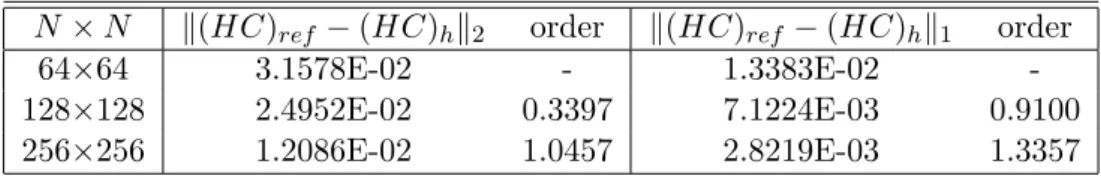
We first carry out the convergence study of the present scheme (18). Here, we perform different computations with varying grid numbers N × N ; N = 64, 128, 256, 512 so the spatial mesh width is h = 2/N . The La-grangian marker width is chosen as ∆s ≈ h/2 and the time step size is ∆t = h/8. The solutions are computed at time T = 0.1. Since the ana-lytical solution is not available in these simulations, we choose the results obtained from the finest mesh as our reference solution and compute the L2

and L₁ errors between the reference solution and the solution obtained from the coarser grid. Table 1 shows the mesh refinement analysis of the bulk concentration in Ω. One can see that the order of convergence is roughly first-order.

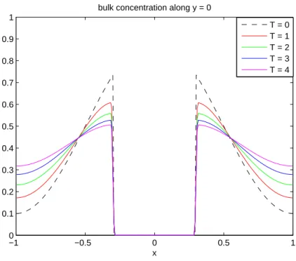
Figure 2 shows the evolutionary bulk concentration along the horizontal line y = 0. One can see that inside the interface, the bulk concentration

N × N k(HC)_ref − (HC)_hk₂ order k(HC)_ref − (HC)_hk₁ order

64×64 3.1578E-02 - 1.3383E-02

-128×128 2.4952E-02 0.3397 7.1224E-03 0.9100

256×256 1.2086E-02 1.0457 2.8219E-03 1.3357

Table 1: The L₂ and L₁ errors and their convergent orders for the bulk diffusion with a fixed interface at T = 0.1.

is almost zero which reflects the insolubility to the region Ω0. Meanwhile,

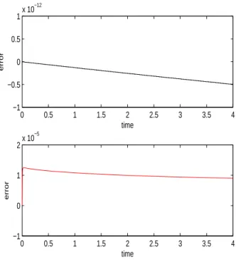
the surfactant diffuses gradually as time evolves in these plots. To see if the total surfactant mass is conserved in the domain, we plot the relative error defined as |Mt−M0|

M0 , where M0 is the initial total surfactant mass while Mtis

the total mass computed at time t. One can see those errors reach machine precision in the upper panel of Figure 3 indicating that the present scheme (18) has the mass conservation exactly.

Although in the plots of Figure 2, the bulk concentration is indistinguish-able zero inside the interface; however, there is still an O(²) amount of mass leaking into the region Ω0due to the regularization of the indicator function.

One can measure the surfactant mass leakage as ML=

P

ij(HC)ijh2 when

Hij ≤ 0.01. In the lower panel of Figure 3, we show the time plots of relative

mass leaking error defined as |ML|

M0 . One can see that the relative error is

within 10−5 _{which is about 0.001%.}

5.2 Bulk convection-diffusion with a moving interface

In this test, we use the same setup as the first test but add the convection effect into the equation. The center of the circular interface is shifted to the point of (0.1, 0) initially so that the asymmetric flow can be developed. The flow and the interface are now moving with a prescribed incompressible velocity field as

u = −1

2(1 + cos(πx)) sin(πy),

v = 1

2(1 + cos(πy)) sin(πx).

Table 2 shows the mesh refinement analysis of the bulk concentration in Ω. One can see that the order of convergence is roughly first-order again even with a moving interface.

−1 −0.5 0 0.5 1 0 0.1 0.2 0.3 0.4 0.5 0.6 0.7 0.8 0.9 1 x

bulk concentration along y = 0

T = 0 T = 1 T = 2 T = 3 T = 4

Figure 2: Time evolutionary plots for bulk concentration along the horizon-tal line y = 0.

N × N k(HC)_ref − (HC)_hk2 order k(HC)ref − (HC)hk1 order

64×64 4.0870E-02 - 1.9293E-02

-128×128 2.4420E-02 0.7429 8.2377E-03 1.2277

256×256 1.1999E-02 1.0251 3.0198E-03 1.4477

Table 2: The L2 and L1 errors and their convergent orders for the bulk

0 0.5 1 1.5 2 2.5 3 3.5 4 −1 −0.5 0 0.5 1x 10 −12 time error 0 0.5 1 1.5 2 2.5 3 3.5 4 −1 0 1 2x 10 −5 time error

Figure 3: Upper panel: total mass relative error versus time. Lower panel: leaking mass relative error inside the interface versus time.

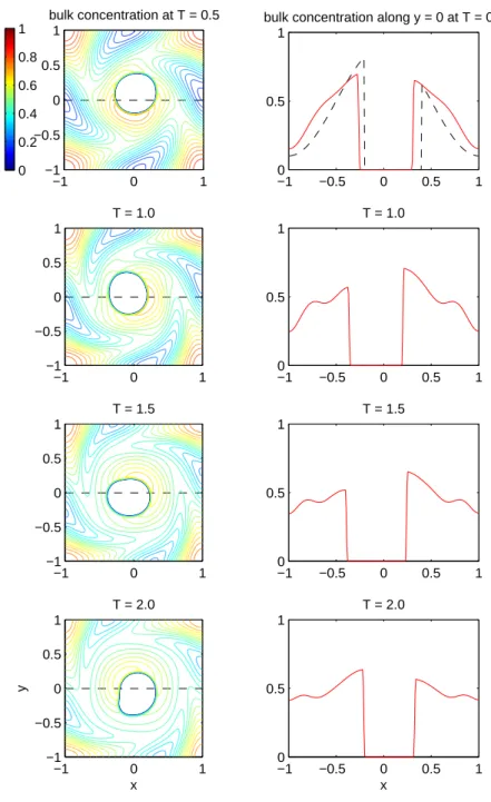
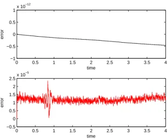
Figure 4 shows the bulk concentration at different times. The left col-umn shows the contour plots of bulk concentration and the instantaneous interface positions. The right column of the figure shows the particular plots along the horizontal line y = 0. One can see that the flow is asymmetric and both convection and diffusion do have apparent effects on the the dis-tribution of bulk concentration. Figure 5 shows the relative errors for total mass in Ω and leaking mass into Ω₀. Again, the total surfactant mass (up-per panel) is conserved almost exactly while the leaking mass error is still controlled within 0.002% Note that, the oscillatory behavior of the latter error is due to the convection of the flow.

5.3 Surface-bulk coupling with a moving interface

In this test, we consider the surface-bulk coupling of the system with a moving interface; that is, we need to solve both equations (17) and (18). Here, we choose the Peclet numbers P e = P es = 100 and the adsorption

and desorption Stanton numbers as Sa = Sd= 1.0. We set the initial bulk

concentration as C₀(x, y) = 0.5(1 − x2₎2 _{so that it satisfies no-flux boundary}

condition along the computational domain Ω = [−1, 1] × [−1, 1]. We also set the initial surface concentration to be identically zero (Γ0(s) = 0) in that

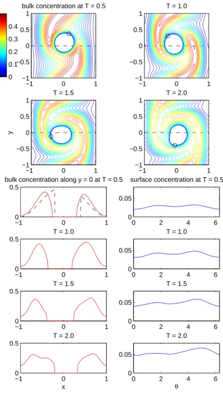
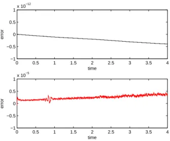
way we shall see some significant surface absorptions near the interface. Figure 6 shows the bulk concentration at different times. The upper panel shows the contour plots of bulk concentration and the instantaneous interface positions. The lower left column of the figure shows the particular bulk plots along the horizontal line y = 0, while the lower right column shows the surface concentration along the interface. Since the total mass is conserved, the bulk concentration is decreasing while the surface concentra-tion increases significantly due to the adsorpconcentra-tion process. The relative errors for total mass in Ω and leaking mass into Ω0 are shown in Figure 7. Again,

the total surfactant mass is conserved almost exactly while the leaking mass error is controlled within 0.0005%

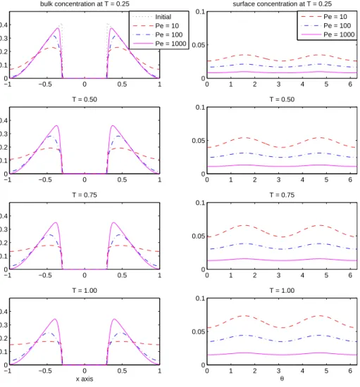
5.4 Surface-bulk diffusion with different Peclet numbers

In this test, we study the diffusion and adsorption effect on different bulk Peclet numbers. We fix the interface and the surface Peclet number P es =

100, but vary the bulk Peclet numbers as P e = 10, 100, 1000. As in the pre-vious test, we set the initial bulk concentration as C0(x, y) = 0.5(1 − x2)2

and the initial surface concentration Γ0(s) = 0. Figure 8 shows the bulk

−1 0 1 −1 −0.5 0 0.5 1 bulk concentration at T = 0.5 0 0.2 0.4 0.6 0.8 1 −1 0 1 −1 −0.5 0 0.5 1 T = 1.0 −1 0 1 −1 −0.5 0 0.5 1 T = 1.5 −1 0 1 −1 −0.5 0 0.5 1 x y T = 2.0 −10 −0.5 0 0.5 1 0.5 1

bulk concentration along y = 0 at T = 0.5

−10 −0.5 0 0.5 1 0.5 1 T = 1.0 −10 −0.5 0 0.5 1 0.5 1 T = 1.5 −10 −0.5 0 0.5 1 0.5 1 T = 2.0 x

Figure 4: The bulk concentration at different times. Left column: the bulk concentration contour plots and the interface positions. Right column: the particular plots along the horizontal line y = 0. The dashed line in the first

0 0.5 1 1.5 2 2.5 3 3.5 4 −1 −0.5 0 0.5 1x 10 −12 time error 0 0.5 1 1.5 2 2.5 3 3.5 4 −0.5 0 0.5 1 1.5 2 2.5x 10 −5 time error

Figure 5: Upper panel: total mass relative error versus time. Lower panel: leaking mass relative error inside the interface versus time.

(right column) at different times. One can see that the adsorption occurs significantly along the interface as time evolves and the maximum are ex-actly occurred at the points where the maximum bulk concentration locate. Moreover, the larger P e is, the less surfactant is adsorbed on the interface since the bulk diffusion is smaller. On the other hand, if the bulk Peclet number is small (the bulk diffusion is large), then the surface concentration is higher. This is because when the bulk surfactant near the interface is ab-sorbed, the neighboring portion will be immediately diffusive into the region so the interface adsorption can be continued. Once can see some apparently different bulk concentration distribution with different Peclet numbers in the left column of Figure 8.

5.5 A freely oscillating drop

We now consider a freely oscillating drop immersed in a quiescent flow as our first test for the numerical scheme described in Section 4. The initial drop interface is an ellipse centered at the origin with major and minor radius 0.6 and 0.15 in a fluid domain Ω = [−1, 1] × [−1, 1], respectively. That is, the initial interface configuration is given as X(s) = (0.6 cos s, 0.15 sin s), 0 ≤ s ≤ 2π. Along the interface, an initial surface concentration is defined as

−1 0 1 −1 −0.5 0 0.5 1 bulk concentration at T = 0.5 0 0.1 0.2 0.3 0.4 −1 0 1 −1 −0.5 0 0.5 1 T = 1.0 −1 0 1 −1 −0.5 0 0.5 1 y T = 1.5 −1 0 1 −1 −0.5 0 0.5 1 T = 2.0 −1 0 1 0 0.5

bulk concentration along y = 0 at T = 0.5

−1 0 1 0 0.5 T = 1.0 −1 0 1 0 0.5 T = 1.5 −1 0 1 0 0.5 T = 2.0 x 0 2 4 6 0 0.05 surface concentration at T = 0.5 0 2 4 6 0 0.05 T = 1.0 0 2 4 6 0 0.05 T = 1.5 0 2 4 6 0 0.05 T = 2.0 θ

Figure 6: Upper panel: the bulk concentration contour plots and the in-terface positions. Lower left: the particular plots along the horizontal line y = 0. The dashed line in the first plot denotes the initial bulk concen-tration. Lower right: the surface concentration along the interface

0 0.5 1 1.5 2 2.5 3 3.5 4 −1 −0.5 0 0.5 1x 10 −12 time error 0 0.5 1 1.5 2 2.5 3 3.5 4 −1 −0.5 0 0.5 1x 10 −5 time error

Figure 7: Upper panel: total mass relative error versus time. Lower panel: leaking mass relative error inside the interface versus time.

Γ(s) = 1 − exp(−1.12 + 0.8 cos(4πs)). There is no flow initially; that is, the initial velocity of Navier-Stokes is set to be zero everywhere. Due to surface tension force, the drop starts to move oscillatory. Here, we compare the insoluble and soluble (only in Ω1) cases, where the latter bulk concentration

is set to be zero initially. The parameters P e = P es = 100 and Sa = Sd=

1.0, the Reynolds number Re = 10, and the Capillary number Ca = 2. Figure 9 shows the comparison between insoluble (denoted by dash-dotted line) and soluble (denoted by solid line) cases for a freely oscillating drop. The upper panel shows the interface positions at different times, while the lower left and right show the bulk concentration along y = 0 (soluble case only) and surface concentration, respectively. As expected, both drops will tend to circular shapes gradually. For the soluble case, since the surface surfactant will be desorbed into the neighboring bulk region (see the bulk concentration), the surface concentration is less than the one of the insoluble case. The surface tension along the interface for soluble case is larger than the one of insoluble case; thus, the drop of soluble case tends to be a circular shape faster than the insoluble case.

−10 −0.5 0 0.5 1 0.1 0.2 0.3 0.4 bulk concentration at T = 0.25 Initial Pe = 10 Pe = 100 Pe = 1000 −10 −0.5 0 0.5 1 0.1 0.2 0.3 0.4 T = 0.50 −10 −0.5 0 0.5 1 0.1 0.2 0.3 0.4 T = 0.75 −10 −0.5 0 0.5 1 0.1 0.2 0.3 0.4 T = 1.00 x axis 0 1 2 3 4 5 6 0 0.05 0.1 surface concentration at T = 0.25 Pe = 10 Pe = 100 Pe = 1000 0 1 2 3 4 5 6 0 0.05 0.1 T = 0.50 0 1 2 3 4 5 6 0 0.05 0.1 T = 0.75 0 1 2 3 4 5 6 0 0.05 0.1 T = 1.00 θ

Figure 8: Surface-bulk diffusion with different Peclet numbers. Left column: the bulk concentration along y = 0. The dashed line in the first plot denotes the initial distribution. Right column: the surface concentration along the interface counter-clockwisely.

−0.5 0 0.5 −0.5 0 0.5 interface position at T = 0.5 −0.5 0 0.5 −0.5 0 0.5 T = 1.0 −0.5 0 0.5 −0.5 0 0.5 y T = 1.5 −0.5 0 0.5 −0.5 0 0.5 T = 2.0 −1 −0.5 0 0.5 1 0 0.5 1

bulk concentration along y = 0 at T = 0.5

−1 −0.5 0 0.5 1 0 0.5 1 T = 1.0 −1 −0.5 0 0.5 1 0 0.5 1 T = 1.5 −1 −0.5 0 0.5 1 0 0.5 1 T = 2.0 x 0 2 4 6 0 0.5 1 surface concentration at T = 0.5 0 2 4 6 0 0.5 1 T = 1.0 0 2 4 6 0 0.5 1 T = 1.5 0 2 4 6 0 0.5 1 T = 2.0 θ

Figure 9: The comparison of insoluble (denoted by ”.-”) and soluble (denoted 24

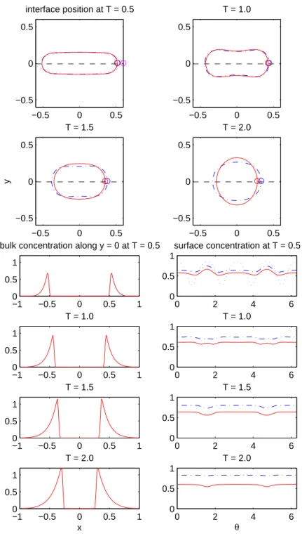
5.6 A drop under shear flow

In the final test, we put a circular drop centered at the origin with radius 0.3 initially in the domain Ω = [−1, 1] × [−1, 1] under the shear flow (u, v) = (y, 0). The initial surface and bulk concentration, the Reynolds number, the Capillary number and other physical parameters are all the same as the previous test.

Figure 10 shows the comparison between insoluble (denoted by dash-dotted line) and soluble (denoted by solid line) cases for a drop under shear flow. The upper panel shows the interface positions at different times, while the lower left and right show the bulk concentration along y = 0 (soluble case only) and surface concentration, respectively. Due to the shear stress, both drops will be elongated and aligned with the flow direction. As in previous test, for the soluble case, the surface surfactant will be desorbed into the neighboring bulk region, so the surface concentration is less than the one of the insoluble case. The surface tension along the interface for soluble case is larger than the one of insoluble case; thus, the drop of soluble case deforms smaller than the one of insoluble case. Moreover, at some point, since the surface tension for the soluble case is stronger than the viscous shear stress, the soluble drop interface will shrink back a little while the insoluble drop interface will be in equilibrium (see the two plots at T = 3 and T = 4 in upper panel). Our numerical results are physically reasonable and qualitative consistent with those obtained in other literature such as in [25].

Acknowledgments

This work was supported in part by National Science Council of Taiwan un-der research grant NSC-98-2115-M-009-014-MY3, NSC-100-2911-I-009-504, and the support of NCTS in Taiwan.

−0.5 0 0.5 −0.5 0 0.5 interface position at T = 1 −0.5 0 0.5 −0.5 0 0.5 T = 2 −0.5 0 0.5 −0.5 0 0.5 y T = 3 −0.5 0 0.5 −0.5 0 0.5 T = 4 −1 −0.5 0 0.5 1 0 0.5

bulk concentration along y = 0

−1 −0.5 0 0.5 1 0 0.5 T = 2 −1 −0.5 0 0.5 1 0 0.5 T = 3 −1 −0.5 0 0.5 1 0 0.5 T = 4 x 0 2 4 6 0 0.5 1 surface concentration at T = 1 0 2 4 6 0 0.5 1 T = 2 0 2 4 6 0 0.5 1 T = 3 0 2 4 6 0 0.5 1 T = 4 θ

Figure 10: The comparison of insoluble (denoted by ”.-”) and soluble (de-26

References

[1] S. Adami, X. Y. Hu, N. A. Adams, A conservative SPH method for surfactant dynamics, J. Comput. Phys. 229 (2010) 1909–1926.

[2] D. Adalsteinsson, J. Sethian, Transport and diffusion of material quan-tities on propagating interfaces via level set methods, J. Comput. Phys. 185 (2003) 271–288.

[3] J. Adams, P. Swarztrauber, R. Sweet, Fishpack- A package of Fortran subprograms for the solution of separable elliptic partial differential equations, 1980. Available in http://www.netlib.org/fishpack.

[4] M. R. Booty, M. Siegel, A hybrid numerical method for interfacial fluid flow with soluble surfactant, J. Comput. Phys. 229 (2010) 3864–3883. [5] M. Burger, Numerical simulation of anisotropic surface diffusion with

curvature-dependent energy, J. Comput. Phys. 203 (2005) 602–625. [6] E. B¨ansch, P. Morin, R. H. Nochetto, A finite element method for

surface diffusion: the parametric case, J. Comput. Phys. 203 (2005) 321–343.

[7] M. Bertalmio, L.-T. Cheng, S. J. Osher, G. Sapiro, Variational problems and partial differential equations on implicit surfaces, J. Comput. Phys. 174 (2001) 759–780.

[8] K.-Y. Chen, K.-A. Feng, Y. Kim and M.-C. Lai, A note on pressure accuracy in immersed boundary method for Stokes flow, J. Comput. Phys. 230 (2011) 4377–4383.

[9] G. Dziuk, C. M. Elliott, Finite element on evolving surfaces, IMA J. Numer. Anal. 27 (2007) 262–292.

[10] G. Dziuk, C. M. Elliott, Surface finite elements for parabolic equations, J. Comput. Math. 25 (2007) 385–407.

[11] C. M. Elliott, B. Stinner, V. Styles, R. Welford, Numerical computation of advection and diffusion on evolving diffuse interfaces, IMA J. Numer. Anal. 31 (2011) 786–812.

[12] F. H. Harlow, J. E. Welsh, Numerical calculation of time-dependent viscous incompressible flow of fluid with a free surface, Phys. Fluids 8 (1965) 2181–2189.

[13] S. Khatri and A.-K. Tornberg, A numerical method for two phase flows with insoluble surfactant, Computers Fluids 49 (2011) 150–165. [14] M.-C. Lai, Y.-H. Tseng and H. Huang, An immersed boundary method

for interfacial flows with insoluble surfactant, J. Comput. Phys. 227 (2008) 7279–7293.

[15] M.-C. Lai, Y.-H. Tseng, H. Huang, Numerical simulation of moving contact lines with surfactant by immersed boundary method, Commun. Comput. Phys. 8 (2010) 735–757.

[16] M.-C. Lai, C.-Y. Huang, Y.-M. Huang, Simulating the axisymmetric in-terfacial flows with insoluble surfactant by immered boundary method, International Journal of Numerical Analysis and Modeling 8 (2011) 105-117.

[17] S. Leung, J. S. Lowengrub, H.-K. Zhao, A grid based particle method for high order geometrical motions and local inextensible flows, J. Comput. Phys. 230 (2011) 2540–2561.

[18] M. Muradoglu, G. Tryggvason, A front-tracking method for computa-tion of interfacial flows with soluble surfactants, J. Comput. Phys. 227 (2008) 2238–2262.

[19] I. L. Novak, E. Gao, Y.-S. Choi, D. Resasco, J. C. Schaff and B. M. Slepchenko, Diffusion on a curved surface coupled to diffusion in the volume: Application to cell biology, J. Comput. Phys. 226 (2007) 1271– 1290.

[20] C. S. Peskin, The immersed boundary method, Acta Numerica, (2002) 1–39.

[21] Y. Pawar, K. J. Stebe, Marangoni effects on drop deformation in an extensional flow: the role of surfactant physical chemistry, I. Insoluble surfactants, Phys. Fluids 8 (1996) 1738.

[22] A. R¨atz, A. Voigt, PDE’s on surfaces - A diffuse interface approach, Commun. Math. Sci. 4 (2006) 575–590.

[23] P. Schwartz, D. Adalsteinsson, P. Colella, A. P. Arkin, M. Onsum, Numerical computation of diffusion on a surface, PNAS 102 (2005) 11151–11156.

[24] K. E. Teigen, X. Li, J. Lowengrub, F. Wang, A. Voigt, A diffuse-interface approach for modeling transport, diffusion and adsorp-tion/desorption of material quantities on a deformation interface, Com-mun. Math. Sci. 7 (2009) 1009-1037.

[25] K. E. Teigen, P. Song, J. Lowengrub, A. Voigt, A diffuse-interface method for two-phase flows with soluble surfactants, J. Comput. Phys. 230 (2011) 375–393.

[26] S. O. Unverdi and G. Tryggvason, A front-tracking method for viscous incompressible multi-fluid flows, J. Comput. Phys. 100 (1992) 25–37. [27] J.-J. Xu, H.-K. Zhao, An Eulerian formulation for solving partial

dif-ferential equations along a moving interface, J. Sci. Comput. 19 (2003) 573–594.

[28] X. Yang, X. Zhang, Z. Li, G.-W. He, A smoothing technique for dis-crete delta functions with application to immersed boundary method in moving boundary simulations, J. Comput. Phys. 228 (2009) 7821–7836. [29] Y. N. Young, M. R. Booty, M. Sigel, J. Li, Influence of surfactant solubility on the deformation and breakup of a bubble or capillary jet in a viscous fluid, preprint.

[30] J. Zhang, D. M. Eckmann, P. S. Ayyaswamy, A front tracking method for a deformable intravascular bubble in a tube with soluble surfactant transport, J. Comput. Phys. 214 (2006) 366–396.