基於H.264的混合式多重描述編碼

國

立

交

通

大

學

資訊科學與工程研究所

碩

士

論

文

基於 H.264 的混合式多重描述編碼

Hybrid Multiple Description Coding Based on H.264

研 究 生：陳建裕

指導教授：蔡文錦 教授

ii

基於 H.264 的混合式多重描述編碼

Hybrid Multiple Description Coding Based on H.264

研 究 生：陳建裕 Student：Jian-Yu Chen

指導教授：蔡文錦 Advisor：Wen-Jiin Tsai

國 立 交 通 大 學

資 訊 科 學 與 工 程 研 究 所

碩 士 論 文

A Thesis

Submitted to Institute of Computer Science and Engineering College of Computer Science

National Chiao Tung University in partial Fulfillment of the Requirements

for the Degree of Master

in

Computer Science

October 2009

Hsinchu, Taiwan, Republic of China

iii

基於 H.264 的混合式多重描述編碼

學生 : 陳建裕

指導教授 : 蔡文錦 教授

國立交通大學

資訊科學與工程研究所

摘 要

當視訊資料透過網路傳輸時，會因為不同的傳輸錯誤，而在視訊品質上產生 負面影響，多重描述視訊編碼就是一種用於降低錯誤影響的技術。在多重描述編 碼上有著許多的方法，都勢必考量到編碼效能與錯誤恢復，並在其中取得一個最 好的平衡點。而在此篇論文中，我們提出了一種混合式的多重描述編碼技術。 在混合式多重描述編碼架構模型上，我們利用了時間域與空間域的特性，將 其視訊來源編碼分割，在使用個別兩個的動作預測迴圈下，以產生四個描述子， 個別在不同頻道上傳輸，其中任一個描述子都可單獨解碼還原，接收端的描述子 收到越多則還原的品質越佳。 當有描述子發生錯誤或遺失時，混合式多重描述編碼會在時間域或空間域上， 錯誤選取較適合的預估方式，結果顯示，可以使得視訊在有效率的編碼效能下， 達到較好的錯誤恢復。在理想頻道上描述子遺失，或在網路隨機封包遺失的情況 下，都可以顯示混合式多重描述編碼的優勢。 關鍵字 : 多重描述編碼、多相重排與次取樣、誤配控制、錯誤隱藏

iv

Hybrid Multiple Description Coding Based on

H.264

Student: Jian-Yu Chen Advisor: Dr. Wen-Jiin Tsai College of Computer Science

National Chiao Tung University

Abstract

Multiple description (MD) video coding is one of the techniques used to reduce the detrimental effects caused by transmission over error-prone networks. Several approaches have been proposed for MD coding, where each provides a different tradeoff between compression efficiency and error resilience. This paper presents a hybrid MD coding method.

The hybrid MD encoder segments the video along both temporal and spatial dimensions, and generates four descriptions using two motion prediction loops. In case of description loss, the hybrid MD decoder adaptively takes advantages of spatial correlation among residual pixels and temporal correlation between frames for lost data estimation. As a result, better error resilience can be achieved at high compression efficiency. The advantages of the proposed hybrid MD method are demonstrated in the contexts of description loss in ideal channels and in packet loss networks.

Keywords: Multiple description coding, Polyphase permutation and sub-sampling,

v

Table of Contents

CHAPTER 1 INTRODUCTION ... 1

1.1 PREFACE ... 1

1.2 MULTIPLE DESCRIPTION CODING... 4

CHAPTER 2 RELATED WORK ... 7

2.1 CLASS AMDCMODEL ... 7

2.2 CLASS BMDCMODEL ... 9

CHAPTER 3 MOTIVATION ... 13

CHAPTER 4 HYBRID MODEL ... 15

4.1 HYBRID ENCODER ... 15

4.1.1 Temporal Splitter ... 16

4.1.2 Residual Splitting ... 17

4.2 HYBRID DECODER ... 19

4.3 ESTIMATION OF LOST DESCRIPTION ... 20

4.3.1 Spatial Estimation Method ... 20

4.3.2 Temporal Estimation Method ... 21

4.3.2.1 Whole Frame Estimation with B-PMVI ... 22

4.3.2.2 Partial Frame Estimation with B-PMVE ... 24

4.3.3 Estimation Method Selection ... 25

CHAPTER 5 EXPERIMENTAL RESULTS ... 32

5.1 PERFORMANCE OF ESTIMATION OF LOST DESCRIPTION ... 32

5.1.1 Temporal Estimation Method ... 33

5.1.2 Spatial Estimation Method ... 34

5.1.3 Adaptive Estimation Method ... 35

5.2 PACKET LOSS PERFORMANCE ... 36

5.3 SIDE RECONSTRUCTION PERFORMANCE ... 42

5.3.1 One Missing Description ... 42

5.3.2 Two Missing Descriptions ... 45

5.3.3 Three Missing Descriptions... 46

CHAPTER 6 CONCLUSION ... 49 REFERENCE 50

vi

List of Figures

FIGURE 1.1 CONVENTIONAL MDC SYSTEM ARCHITECTURE. ... 4

FIGURE 2.1 ENCODER SYSTEM ARCHITECTURE OF [6]. FROM [6] ... 8

FIGURE 2.2 INDEX ASSIGNMENT OF SCALAR QUANTIZER. FROM [6] ... 8

FIGURE 2.3 PSS SYSTEM ARCHITECTURE... 11

FIGURE 2.4 POLYPHASE SUB-SAMPLING... 11

FIGURE 2.5 PATTERN FOR RECEIVING THREE DESCRIPTORS. ... 12

FIGURE 4.1 ENCODER OF HYBRID MDC ... 15

FIGURE 4.2 HYBRID ENCODER ARCHITECTURE... 16

FIGURE 4.3 POLYPHASE PERMUTING OF A 8X8 BLOCK ... 17

FIGURE 4.4 SPLITTING OF A 8X8 BLOCK ... 18

FIGURE 4.5 DECODER OF HYBRID MSC ... 19

FIGURE 4.6 HYBRID DECODER ARCHITECTURE... 20

FIGURE 4.7 SPATIAL CONCEALMENT BY BILINEAR INTERPOLATION ... 21

FIGURE 4.8 B-PMVI BIDIRECTIONAL ESTIMATION. ... 23

FIGURE 4.9 B-PMVI MOTION VECTOR INTERPOLATION. ... 23

FIGURE 4.10 B-PMVE BIDIRECTIONAL ESTIMATION. ... 24

FIGURE 4.11 B-PMVE MOTION VECTOR INTERPOLATION. ... 25

FIGURE 4.12 ‘S→T’ FOR THREE MISSING DESCRIPTIONS. ... 27

FIGURE 4.13 TEMPORAL ESTIMATION FOR TWO MISSING DESCRIPTIONS FROM THE SAME PREDICTION LOOP. ... 27

FIGURE 4.14 ADAPTIVE SELECTION OF ESTIMATION METHODS. ... 28

FIGURE 4.15 RELATION BETWEEN PSNR AND GRADIENT VALUE. ... 30

FIGURE 4.16 RELATION BETWEEN PSNR AND ADJUSTED GRADIENT VALUE. ... 31

FIGURE 4.17 RELATION BETWEEN Σ AND QP ... 31

FIGURE 5.1 TEMPORAL ESTIMATION METHODS USED FOR COMPARISON ... 33

FIGURE 5.2 PERFORMANCE COMPARISON IN PACKET-LOSS ENVIRONMENT (SEQUENCE WITH GOP30). ... 39

vii

FIGURE 5.3 PERFORMANCE COMPARISON IN PACKET-LOSS ENVIRONMENT

(SEQUENCE WITH GOP300). ... 41

FIGURE 5.4 PSNR DEGRADATION OF PACKET LOST IN 40TH FRAME. ... 42

FIGURE 5.5 PSNR OF ONE DESCRIPTION LOSS FOR DIFFERENT BIT-RATE. ... 44

FIGURE 5.6 PSNR OF TWO DESCRIPTION LOSS FOR DIFFERENT BIT-RATE. ... 46

viii

List2 of Table

TABLE 1-1 BENEFITS OF ERROR RESILIENCE TOOLS ACCORDING TO CATEGORY. FROM [1]. ... 2 TABLE 4.1 SUMMARY OF ESTIMATION METHODS IN THE CORRESPONDING CASES.

... 26 TABLE 5.1 PSNR OF DIFFERENT TEMPORAL ESTIMATION METHODS (PARTIAL

FRAME LOSS). ... 34 TABLE 5.2 PSNR OF DIFFERENT SPATIAL ESTIMATION METHODS. ... 35 TABLE 5.3 PERFORMANCE OF ADAPTIVE ESTIMATION. ... 35

1

Chapter 1

Introduction

Introduction

1.1 Preface

Through the growing of the communication technology, video streaming has recently become a popular field. There had been more and more application services about video streaming being developed and provided, such as, IPTV, peer-to-peer (P2P) live video and video phone; the scale of these services also becomes larger. Transmitting video streams smoothly to effectively combat network errors is an important subject.

H.264/AVC is one of the most newly introduced video coding standard developed by Joint Video Team founded by ITU-T and ISO/IEC, which has a better video quality and compression efficiency than existing standards, such as MPEG2 and H.263. When transmitting the H.264/AVC encoded bit-stream, as the coding efficiency is higher, the bits of the encoded stream carry more information of the video source, and the bit-stream would be more vulnerable to transmission errors. As a result, there had been a lot of error resilience tools proposed to combat transmitting error; table 1.1 from [1] by A. Vetro, J. Xin and H. Sun summarizes recently proposed error resilience tool. These tools are classified into four different groups according to field of categories and their benefits are listed separately. Localization is a technique that can restrain the error to propagate in a limit range; data partitioning separates the

2

encoded bit-stream into different parts, each has unequal importance so that one can protect each part with different levels of security; redundant coding protects the bit-stream with additional data bits, that is when error occurs, the correctly received parts can be used to recover the lost parts; concealment-driven aims to predict lost part of data with the aid of correlation on either spatial or temporal domain. H.264/AVC had incorporated almost all tools in the four categories from table 1.1: 1) adaptive intra refresh; 2) reference picture selection; 3) multiple reference pictures; 4) data partition of MV, header and texture; 5) Redundant slice; 6) Flexible macroblock order.

Table 1-1 Benefits of error resilience tools according to category. From [1].

Low-bandwidth handheld devices have become more popular and backbone capacities of the Internet has increased, thus for a video streaming service, the client bandwidth varies in a wide range, from hundreds of kilo-bytes to tens of mega-bytes. Clients on hand-held devices such as cell phone, smart phone or PDA, usually have lower bandwidth, while in desktop, higher bandwidth is common. As a result, a service that is adaptive to the varying bandwidth of heterogeneous networks would become more appealing.

3

Real-time is another important characteristic in video streaming services. A system that utilizes retransmission or feedback channel may result in an unacceptable delay; since retransmitting lost packets would add at least one round-trip time delay, thus the packet would expired its display timeline.

In the streaming on P2P network, the receiving of data stream may come from different source peers through different paths, and the path may failed if one peer along the path failed, thus the receiver could constantly losing part of data from some peers. As the failure of peer is not predictable, the part of data which will get lost during transmission is not know a priori. In this circumstance, using unequal error protection would not be effective. If receivers can make use of whatever they received and utilize the appropriate error concealment and/or resilience tools, the system will have a better performance.

Thus, to successfully transmit video stream in heterogeneous error prone networks, we expect that the video streaming system should at least have the following requirements:

1. Scalable bandwidth and quality

 The receivers can be classified into groups by the capability of its bandwidth and display quality; the higher bandwidth, the better quality. 2. Equal protection on each part of data

 To simplify the transmitting mechanism, each part of data is treated equally.

3. Avoiding feedback channel and retransmission

 Waiting for the feedback and retransmit the lost packet could imposes a unacceptable delay while playing video

4. Error resilience function

4

Multiple description coding (MDC), in the “Redundant coding” category in table 1.1, is a technique that meet the above criterions.

1.2 Multiple Description Coding

MDC is a technique that encodes a single information source into two or more output streams, called descriptors, and each descriptor can be decoded independently and has an acceptable decoding quality; in addition, the decoding quality will be better if more descriptors were received. Contrary to MDC, single description coding (SDC) is used to indicate the standard encoded bit-stream with H.264/AVC.

MDC is first originated from an interesting problem from information theory: If an information source is described with two separate descriptions, what are the concurrent limitations on qualities of these descriptions taken separately and jointly? [2]. This problem was first presented by Wyner and latter became the MD problem. Latter in 1993, Vaishampayan had proposed the first practical implementation of MD, called multiple description scalar quantizer(MDSQ) [4], which proposes two index assignment table: nested index assignment and linear index assignment, that map a quantized coefficient into two indices each could be coded with fewer bits. Afterwards, researches on different implementations of MDC had been proposed, and will be introduced later.

5

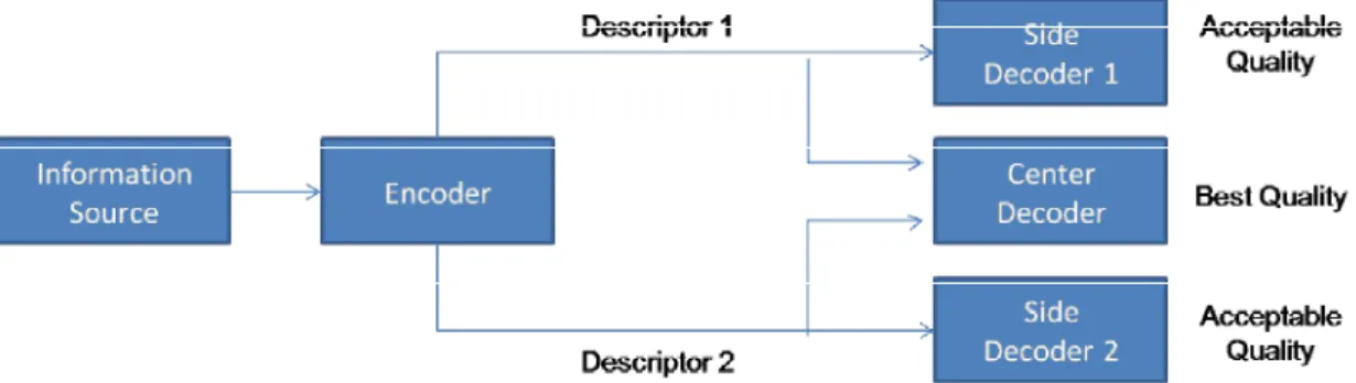
Most MDC approaches focus on how to generate two descriptors so that each descriptor would have good decoding quality and the overall two channel bit-rate would be minimized. Figure 1.1 shows the conventional MDC system architecture. The encoder encodes the source into two individual descriptors and then sends through two channels. The decoder has multiple decoder states: side decoder and center decoder; when receiving only one descriptor, the side decoder will be responsible to decode the one descriptor bit-stream; if both descriptors were received the center decoder will produce the best quality output.

Layered coding, such as scalable video coding(SVC), is a technique that encodes the bit-stream into base layer and enhancement layers; base layer has lower bit-rate and a basic acceptable quality of video, and enhancement layers are used to refine the video quality. If the network traffic is congested, the receiver can receive only base layer; if the bandwidth is sufficient for the receiver to obtain more data, the enhancement layers will be used to further refine the decoding quality. The more enhancement layers are received, the better the decoding quality can be obtained.

SVC seems to meet the four requirements mentioned in section 1.1 and has similar features with MDC, but they are different in the view of data importance: SVC treats base layer more important, while the descriptors are equally important in MDC. The different importance of base layer and enhancement layers are due to the fact that enhancement layers cannot be reconstructed without the base layer. In other words, if the base-layer data packets are corrupted, then the corresponding enhancement layers’ data packets will be useless. Contrary to SVC, each descriptor of MDC has equal importance, bit-rate and quality. Consider the case that the information source are encoded into n descriptors in MDC architecture, while in SVC, n-1 enhancement layers and one base layer are generated. In both systems the resulting bit-streams are sent through n separate channels and each channel has average error probability p.

6

Then, the probability that the receiver can reconstruct the video is: 1) 1-p, for SVC; 2) 1-pn, for MDC. In conventional error prone environment, for example, wireless network, the average error rate p might be 20%, and let n = 2, then the probability to successfully reconstruct the video for MDC is 0.96 (1-0.04), which is higher than 0.8 (1-0.2) for SVC.

7

Chapter 2

Related Work

Related Work

There have been a lot of MDC models proposed since the first implementation, MDSQ [4]. These models can be intuitively classified through the stage where it split the original signal, such as, spatial domain, frequency domain and temporal domain. To be more precisely, in [3], Wang had come up with another classification approach, that is based on the type of predictor a MDC model had adopted and three classes have been defined. Class A focuses on the prediction efficiency; class B focuses on the mismatch control; and Class C controls trade-off between the two issues. Since the performance evaluation of the proposed model will be compared to the models from class A and B, the following sections describe the two models in details.

2.1 Class A MDC Model

MDC models of Class A have the property that the predictor used in the encoder is in accordance with that used in SDC, which has the best prediction efficiency, in other words, the prediction of class A encoder is the same as the center decoder. In motion estimation, the reconstructed reference frames is fully reconstructed in the encoder as if all descriptors are received in the decoder, thus the predictor can find the most similar regions in the reference frames. As a result, the prediction efficiency is efficient using class A.

8

The first implementation of MDC, MDSQ [4], focuses on splitting general signal source, and latter in [6] had applied the MDSQ approach to H.264/AVC. Figure 2.1 shows the encoder architecture proposed in [6]. It can be observed that it is a typical class A architecture because there is only one prediction loop, and after quantization, the coefficients are split to two paths, generating two descriptors, NAL 1 & NAL 2.

Figure 2.1 Encoder System Architecture of [6]. From [6].

The function of MDSQ block in Figure 2.1 is illustrated in Figure 2.2, where the numbers in the 2D array are quantized DCT coefficients, and each one is mapped to two indexes in vertical and horizontal directions.

9

There are a number of class A models based on splitting either frequency coefficients or residual data. In [8], the transformed coefficients are split to two descriptors such that the total distortion and bit-rate of two descriptors are minimized by Lagrange multiplier λ. Even though the generated descriptors have optimal total distortion, the reconstruction quality and bit-rate of descriptors are different, resulting in unbalanced descriptors. In [9], a balanced splitting of coefficients is proposed to combat this issue, in which the splitting process is divided to two stages. First, the coefficients are assigned to two descriptors so that the difference of energy between two descriptors are minimized, which resulting in balanced distortion. Then, the coefficients are swapped to make sure the two descriptors have a nearly the same bit-rate. [10] is another MDC model of class A. It is more flexible in that two or three descriptors can be generated and is also based on frequency coefficients splitting. In [11], the splitting is based on prediction error. The residual of each macroblock after motion compensation is polyphase permuted and the split to two descriptors. Then, a new data partition mode is added to generate two descriptors

2.2 Class B MDC Model

The main characteristic of class B models is prediction mismatch control, which is achieved by taking the state of decoder into account. The prediction in the encoder of class B is the same as that in the side decoder of each descriptor, in other words, it can be viewed as encoding the descriptors separately so that when decoding any one descriptor, the prediction for every macroblock is the same as that in encoder, resulting in better quality compared with class A model in case of descriptor loss. Using class A model, the worse reconstructed quality is due to the loss of partial information used for prediction in the decoder. Thus, the main difference between

10

class A and class B models is that what information is used for prediction.

In class B, the information used for prediction falls into two types: one uses partial information contained in each descriptor for prediction; the other uses the information common in every descriptor for prediction. However, both of these two types result in prediction inefficiency: incomplete information is used for prediction, so that the predicted blocks used may not be the same as those in SDC, resulting in a larger prediction error. Hence, the bit-rate increased for a given quality.

A variety of MDC approaches adopt class B model, from simple to complex architectures. The simplest approach might be the one that splits the video sequence to odd and even frames, separately encodes the two groups to form two descriptors and applies error concealment in the side decoders [12]. The prediction inefficiency is increased when the temporal distance is increased. Therefore, if three or more descriptors are to be generated, the prediction for each descriptor becomes more inefficient. In [13], a more complex architecture is proposed. Two type of frames, H-SNR for high quality and L-SNR for low quality, are alternative placed in two descriptors, and two-stage quantization is used. H-SNR frames are produced in the 1st stage and L-SNR frames are produced in the 2nd stage quantization. The mismatch control is done by using the L-SNR frames as reference frames, since H-SNR could be transformed to L-SNR for the 2nd stage quantization in the decoder. This model is an example of class B with the type that uses information common in both descriptors for prediction. [14] is another class B model based on H.264/AVC. It utilizes the slice group with disperse mode which groups macroblocks in a frame to two slices and forms a check board pattern. In one descriptor, one of the two slices is quantized by a higher quantization parameter (QP) and the other with a lower QP, and in the other descriptor, the QP is reversed. Since lower QP has higher quality, if two descriptors are all received, the lower QP slices in each descriptor is displayed; while if only one

11

descriptor is received, the two slices, on high Qp and on with low QP, in this descriptor are displayed.

The polyphase spatial sub-sampling (PSS) model [7] is designed for generating four descriptors, and will be used for comparison with the proposed model. The encoder and decoder used in [7] is a conventional H.264/AVC encoder and decoder. The splitting is done before the encode and the merging is done after the decoder, as shown in Figure 2.3.

Figure 2.3 PSS System Architecture.

The “Polyphase Splitter” splits each frame of the original sequence to four sub-frames, each has half size of width and height. The process is shown in Figure 2.4, where the left 4x4 block is assumed to be the original frame with resolution 4x4, and first sub-sampled by factor 2 row-by-row and then column-by-column.

12

There are totally 14 cases of the received descriptors: four case for one descriptor; six cases for two descriptors; four cases for three descriptors. After receiving descriptors from network, each descriptor is decoded separately by standard H.264/AVC decoder, and then the received descriptors are merged and the lost descriptors are concealed. In [7], A non-linear interpolator, called edge sensing, is proposed for error concealment in the case of receiving three descriptors, while in other cases a conventional bilinear interpolator and near neighbor replicator (NNR) is used for the concealment. The edge sensing algorithm is based on gradient calculation of the lost pixels. Figure 2.5 illustrates the pattern of receiving three descriptors. Y0 is to be predict by Y1, Y3, Y5 and Y7, and two gradients will be calculated in x and y directions. With the two gradients, the more smooth direction can be determined, and averaging the pixels in this direction has a better concealment effect than using a bilinear interpolator.

13

Chapter 3

MOTIVATION

Motivation

As the Internet backbone capability increases and more and more hand-held devices connect to network, the Internet becomes much more heterogeneous. A video streaming service may serve for a variety of clients such as PDA or desk-top on different type of networks, such as wired or wireless network. With different types of networks, the bandwidth varies from Kilo-bytes to Mega-bytes. In the MDC architecture, if the number of descriptors increases, the quality and bit-rate thus span a wider range. For example, if four descriptors are generated, the low bandwidth client can receive only one descriptor, while clients with highest bandwidth can receive all four descriptors. The low bandwidth client only needs one quarter bit-rate for the service.

Class B MDC architecture has the characteristic that the side decoders have fully mismatch control, which implies that the encoder prediction loop should take the state of decoder into account, and has less prediction efficiency as discussed in chapter 2. Thus prediction error will become larger and the total redundancy of descriptors will also rise. Further, class B might also need more encoding time, to be more specific, the motion estimation. Since the prediction for each descriptor is different, and motion estimation is needed for each descriptor, the motion estimation time could be linearly depending on the descriptor number. In other words, if more descriptors were

14

generated, more motion estimation time is needed. As a result, to fast split the source into multiple descriptors, say four, with lower redundancy, the class A architecture with splitting on the prediction error approach is a good candidate, because only one motion estimation time is needed and the prediction efficiency could be as well as SDC.

According to the two considerations mentioned above: 1) higher number of descriptors; 2) more efficient encoding time and redundancy; we would like to propose a novel MDC model with class A architecture, that has one motion estimation time and split the source based on prediction error, and extend conventional 2-descriptor MDC approaches to generate four descriptors in order to make the proposed model more adaptive to the clients from heterogeneous networks.

15

Chapter 4

HYBRID MODEL

Hybrid Model

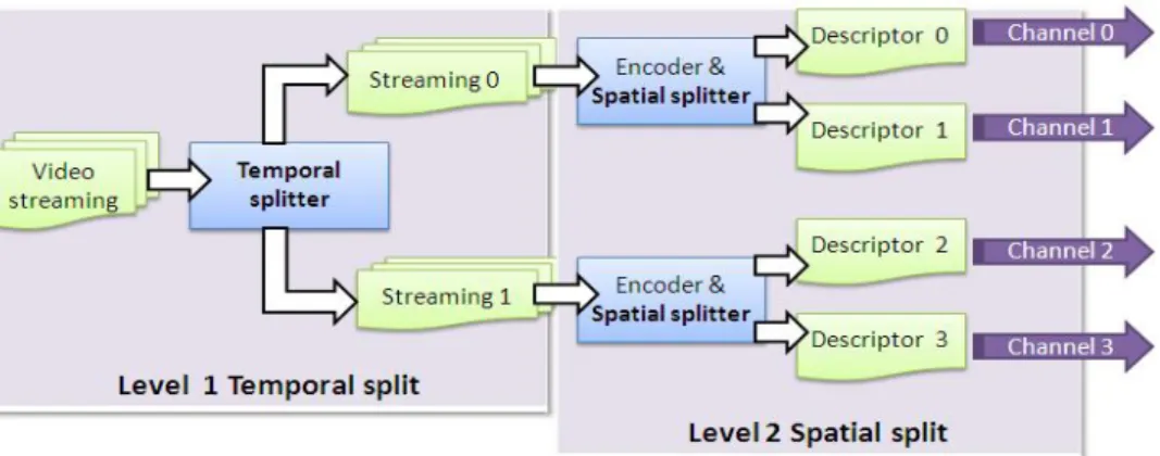
The proposed hybrid model (called Hybrid) combines class- A and class-B methods to generate four descriptions using two motion-estimation prediction loops. It is designed to explore both the temporal correlation between successive frames and the spatial correlation between adjacent motion-compensated residual pixels. In this chapter, the Hybrid encoder is presented first, and then is the Hybrid decoder.

4.1 Hybrid Encoder

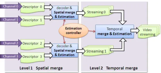
The Hybrid encoder architecture is illustrated in Figure 5.1 & Figure 5.2, where the encoder has a two-level splitting process in the encoding loop: 1) Temporal splitter, and 2) Residual Splitter; the former one is a class-B method which splits the video sequence in temporal domain; while the latter one is a class-A method which splits the motion compensated residual in spatial domain.

16

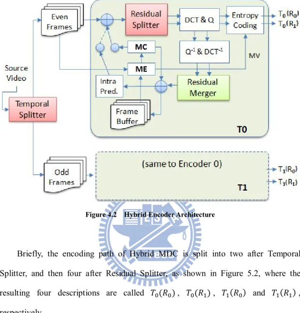
Figure 4.2 Hybrid Encoder Architecture

Briefly, the encoding path of Hybrid MDC is split into two after Temporal Splitter, and then four after Residual Splitter, as shown in Figure 5.2, where the resulting four descriptions are called ( ) , ( ) , ( ) and ( ) , respectively.

4.1.1 Temporal Splitter

The 1st level splitting, Temporal Splitter, splits a sequence along temporal dimension into two subsequences: one for all the even frames and the other for all the odd frames. Even frames are predicted from even ones, and odd frames from odd ones, resulting in two motion-estimation prediction loops. We refer to one of the prediction loops as T0 and the other as T1.

17

4.1.2 Residual Splitting

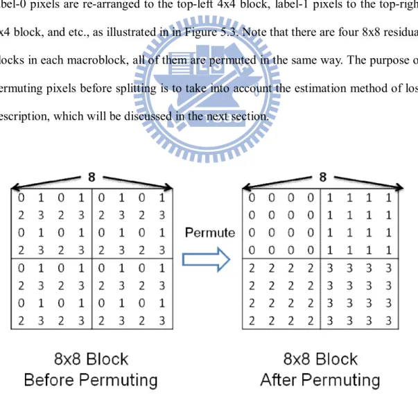
After motion estimation and compensation in each loop, the 2nd level splitting, Residual Splitter, is performed on an 8x8-block basis using polyphase permuting and splitting in the residual domain.

Each motion-compensated 8x8 residual block is first polyphase permuted inside the block and then split to 2 blocks, as shown in Figure 5.3 & Figure 5.4. The permuting mechanism is that the pixels in the 8x8 residual-block are first labeled with numbers ranging from 0 to 3, where for every 2x2 pixels, 0 is labeled on top-left pixel, 1 on top-right pixel, 2 on bottom-left pixel, and 3 on bottom-right pixel; and then label-0 pixels are re-arranged to the top-left 4x4 block, label-1 pixels to the top-right 4x4 block, and etc., as illustrated in in Figure 5.3. Note that there are four 8x8 residual blocks in each macroblock, all of them are permuted in the same way. The purpose of permuting pixels before splitting is to take into account the estimation method of lost description, which will be discussed in the next section.

18

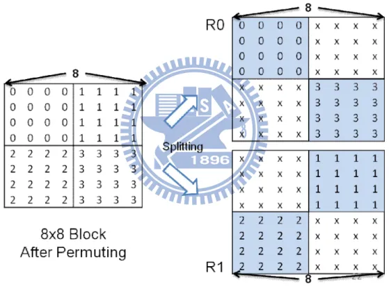
After polyphase permuting, the splitting process is performed to split each 8x8 block into two 8x8 blocks, called residual 0 (R0) and residual 1 (R1), each carries two 4x4 blocks chosen in diagonal: top-left and bottom-right 4x4 blocks belong to one 8x8 block, while top-right and bottom-left ones belong to the other 8x8 block. For each 8x8 block, the remaining two 4x4 blocks with pixels all labeled with ‘x’ in the Figure 5.4 are given residual pixels all set to zero. The encoder has no need to encode the coefficient of these two all-zero 4x4 blocks.

Figure 4.4 Splitting of a 8x8 Block

Note that the 2nd level splitting, Residual Splitter, is a class-A method, which uses a single prediction loop for two descriptions. To construct reference frames for prediction, Residual Merger is used. As shown in Figure 5.2, after de-quantization and inverse transformed, R0 and R1 are obtained and then Residual Merger is applied, which first discards the all-zero 4x4 blocks in R0 and R1, combines the resulting R0

19

and R1 into 8x8 blocks, and then performs polyphase inverse permuting to reconstruct the 8x8 blocks as reference. The four 8x8 blocks in a macroblock are all processed in this way. Actually, the Residual Merger is the reverse of Residual Splitter because it performs polyphase permuting and splitting in a reversed way.

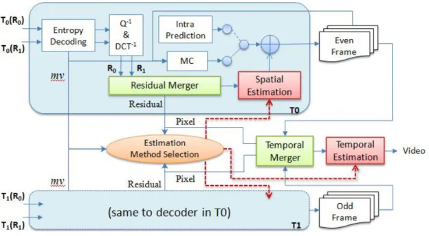
4.2 Hybrid Decoder

Hybrid decoder architecture is depicted in Figure 5.5 & Figure 5.6, where the four input descriptions are ( ), ( ), ( ) and ( ). These descriptions are separately entropy decoded, dequantized, and inversely transformed, and then Residual Merger is applied to merge every two descriptions from the same prediction loops. The Residual Merger adopts residual merging and polyphase inverse permuting in the same way as illustrated in the encoder side. After motion compensation on each prediction loop, the Temporal Merger is applied to reconstruct the whole sequence. As shown in Figure 5.6, lost descriptions (if any) can be spatially estimated after Residual Merger is performed, or be temporally estimated after Temporal Merger is done.

20

Figure 4.6 Hybrid Decoder Architecture

4.3 Estimation of Lost description

Ifthe decoder does not receive all the descriptions intact, then temporal or(and) spatial estimation method of lost description is adopted to reconstruct the lost data. We first describe the spatial estimation and temporal estimation methods used in our Hybrid MDC, and then the selection of estimation methods is presented.

4.3.1 Spatial Estimation Method

Spatial estimation method explores the spatial correlation between residual pixels to estimate the lost description from the same prediction loop, which requires that at least one of the two descriptions split from the same prediction loop is correctly received. As an example, assuming that ( ) and ( ) are two descriptions split from frame n belonging to prediction loop T0, and that ( ) is lost during transmission, to reconstruct the missing ( ), the receiver will apply

21

spatial estimation method only when ( ) is correctly received. After the polyphase inverse permutation of ( ), the residual pixels are distributed like a checkerboard within a macroblock as shown in Figure 4.7, where for each lost residual pixel, four neighboring pixels are available.

Figure 4.7 Spatial Concealment by Bilinear Interpolation

, = , + , + , + , ⁄4

(4.1)

The spatial estimation method uses bilinear interpolation to reconstruct the lost residual pixels, as shown in Equation (4.3) where _, is the reconstructed value of the residual pixel in column i and row j. Since neighboring pixels have high spatial correlation, spatial estimation should be efficient.

4.3.2 Temporal Estimation Method

Temporal estimation method will be applied to recover a whole frame or part of a frame. Here two bi-directional temporal estimation methods are proposed: one uses pixel-based motion vector interpolation (B-PMVI), and the other uses pixel-based motion vector extrapolation (B-PMVE).

22

4.3.2.1 Whole Frame Estimation with

B-PMVI

When two descriptions from the same prediction loop are lost, it will result in the whole-frame loss. Since the proposed Hybrid method splits consecutive frames into different prediction loops, the lost frame can be estimated by its previous frame and next frame in the other prediction loop, as illustrated by the example in Figure 4.8, where assume frame n from prediction loop T1, is lost. Since the MVs of all the MBs in frame n are lost, the lost motion information can be simply replaced by zero, that is, each missing pixel is estimated by the co-located pixel value in the previous decoded frame. This works well for stationary areas, but fails for moving area. Motion vector extrapolation (MVE) [19] is another method combating the frame loss. In this method, the MVs of MBs are extrapolated from the last decoded frame to the missing frame. This method can overcome the disadvantage of incorrect MB displacement, but the block-based MV is too rough to cause block-artifacts. To overcome this problem, Chen proposed a pixel-based MVE method, called PMVE[20], which extended the MVE to pixel level and improved the performance in large motion scenes. However, since PMVE is designed in the context of single description coding (SDC), it only utilizes the pixels in the previous decoded frame for error concealment. In this paper, we take advantage of the proposed Hybrid MDC method and propose a bi-directional pixel-based motion vector interpolation (B-PMVI) method, which replaces the pixels of the lost frame with the average of pixels at motion-compensated locations in two frames coming from the other prediction loop. Let mvi, j denote the motion vector

pointing to frame j from frame i. In Figure 4.9, by interpolating the mvn+1, n-1, an

interpolated block on the missing frame n, and its two interpolated motion vectors, mvin, n-1 and mvin+1,n , can be obtained (Note the interpolation is done at pixel level, so

23

the interpolated block is unnecessary aligned on MB positions). By inversing mvin+1,n ,

we yield two estimated motion vectors for each pixel of the interpolated block: one is forward vector, (fx , fy) = mvin, n-1, and the other is backward vector, (bx,by) =mvi-1n+1, n .

Figure 4.8 B-PMVIbidirectional estimation.

Figure 4.9 B-PMVI motion vector interpolation.

The interpolation is performed for every MV in frame n+1, and the pixels in the lost frame n can be divided into two parts:

 For the pixel covered by at least one interpolated block, its two motion vectors are estimated by averaging the corresponding motion vectors of all overlapped blocks.

 For the pixel not covered by any interpolated block, its two motion vectors are set to zero, i.e., (fx , fy)= (bx,by)=(0, 0).

As a consequence, for a pixel (x, y) in the lost frame n, with its two motion vectors, (fx , fy) and (bx,by), its value Pn(x, y) can be estimated as follows:

24

( , ) = × + , + + ( − ) × + , +

(4.2) Where w is used to adjust the weights of forward and backward motion compensated pixels. In this paper, we simply average the two candidates, i.e., w = 0.5.

4.3.2.2 Partial Frame Estimation with

B-PMVE

When only one description is missing, it will result in partial frame loss. Since the 2nd level splitting of the Hybrid MDC splits a frame in residual domain of the same prediction loop, the resulting two descriptions will have the same motion vectors. Thus, when one of them is lost, its motion vectors can be found in the other one and therefore, motion compensation from its reference frame (if not lost) still can be done. To recover the lost residual data, its reference frame and the next frame in the other prediction loop will be used as depicted in Figure 4.10, where assume one description of frame n is lost. For a lost residual pixel on frame n, since its motion vector pointing to its reference frame is available (i.e., mvn, n-2), the only problem is to

find its motion information on frame n+1. We use motion vector extrapolation (MVE), as depicted in Figure 4.11. By extrapolating mvn, n-2, an extrapolated motion vectors,

mven+1, n can be obtained.

25

Figure 4.11 B-PMVE motion vector interpolation.

That is, for a lost residual pixel (x, y) on frame n, we have its forward motion vector as (fx , fy) = mvn, n-2, and the backward vector as (bx,by) =mve-1n+1, n. With the

two motion vectors, its value Pn(x, y) can be estimated as follows:

( , ) = × + , + + ( − ) × + , +

(4.3) where w is again the weights of forward and backward motion compensated pixels.

4.3.3 Estimation Method Selection

The proposed Hybrid MDC segments a video sequence into four descriptions. There are 16 states of the four descriptions as listed in Table 4.1, where the columns describe the four possible cases for the two descriptions split from prediction loop T0; while the rows describe those for T1. The estimation method to be applied for each case are also shown in this table, where ‘T’ denotes the temporal estimation, and ‘S’ the spatial estimation. The ‘S→T’ denotes that spatial method will be performed first and then temporal method is applied; and the ‘A’ indicates that either temporal or spatial method will be applied but the choice of the method adaptively depends on the content of the video. The ‘N/A’ means no estimation method will be applied. As can be seen in the table, ‘S→T’ is applied only for the cases of three-description loss;

26

while ‘T’ is applied only when two descriptions split from the same prediction loop are lost and the other two are received, that is, the whole frame is lost. For whole frame, temporal method of B-PMVI is used. For other cases, ‘A’ will be applied.

Table 4.1 Summary of estimation methods in the corresponding cases.

Since the Hybrid method splits every two frames into four descriptions using two prediction loops, for consecutive two frames, n and n+1, we refer to their prediction loops as T0 and T1, respectively; and refer to the two descriptions split from frame n as ( ) and ( ); while the other two from frame n+1 as ( ) and ( ). To illustrate the cases that ‘S→T’ will be applied, Figure 4.12 (a) depicts one of the four possible cases that three descriptions are lost. The descriptions marked with ‘(x)’ mean they are lost. In this case, since ( ) from prediction loop T0 is received, spatial estimation can be applied to reconstruct its counterpart, ( ), as indicated by the dotted arrow labeled with ‘S’. After merging ( ) and ( ), the reconstructed frame , together with the backward frame , are used by temporal method B-PMVI to recover the lost whole frame , as indicated by the dotted arrow with ‘T’. Figure 4.12 (b) shows how the ‘S→T’ is performed.

27

(a) Three description loss (b) Spatial and then temporal estimation Figure 4.12 ‘S→T’ for three missing descriptions.

To illustrate the cases that ‘T’ will be applied, Figure 4.13 (a) and Figure 4.13 (b) depict two possible cases that two descriptions from the same prediction loop are lost. In either case, spatial estimation method cannot be applied because the lost description has no counterpart from the same prediction-loop available for spatial estimation. For these cases, temporal method of B-PMVI will be applied for whole frame estimation. For example in Figure 4.13 (a), after merging and polyphase inverse permuting, the full frame from prediction loop T0 can be obtained, which is then adopted by temporal estimation to recover the lost frame belonging to prediction loop T1.

(a) Two descriptions of T1 are lost (b) Two descriptions of T0 are lost.

Figure 4.13 Temporal estimation for two missing descriptions from the same prediction loop.

28

different prediction loops are lost or when there is only one-description loss, as those labeled by ‘A’ in Table 4.1. Figure 4.14 (a) depicts one out of four possible cases that one description is lost, and Figure 4.14 (b) shows one of four possible cases that two descriptions from different prediction-loops are lost. Note that, in these cases, since each lost descriptor can obtain correct motion vectors from the counterpart of the same prediction loop, motion compensation is able to be performed without estimation. Thus, only lost residual data needs to be estimated. For these cases, adaptive method which could be either spatial estimation or temporal estimation of B-PMVE will be applied. As an example in Figure 4.14 (a), the missing residual of ( ) can be predicted either from ( ) by using spatial estimation, or from two frames, and , by using temporal estimation method, B-PMVE. In Fig. 11(b), the lost residual of ( ) and ( )can also be predicted either by spatial or temporal methods in a similar way aforementioned.

(a) One description is lost

(b) Two descriptions from different prediction loops are lost Figure 4.14 Adaptive selection of estimation methods.

29

Intuitively, it is more beneficial to adopt spatial estimation if it is a simple textured and high-motion video; and to apply temporal estimation if it is a slow-motion and complex textured video. To effectively select appropriate estimation methods for the above cases, a content- adaptive method is designed for the decoder, which measures the gradient of the lost residual pixels along the spatial and temporal dimensions to determine the characteristic of the video content and then makes the choice.

The spatial gradient (GS) of a residual pixel is calculated as the average of the difference between its two adjacent residual pixels in horizontal direction and that in vertical direction. Let rn(i, j) denote a residual pixel at (i, j) of frame n. The spatial

gradient of this residual pixel is defined as:

( , )= ( , )− ( , ) + ( , )− ( , ) (4.4) The temporal gradient (GT) of a pixel is measured as the difference between the motion-compensated pixel in reference frame and the pixel at extrapolated location in the next frame, where pixel values, instead of residual-pixel values, are used in the calculation. For a residual pixel at (x, y) of frame n, assume its forward and backward motion vectors are (fx , fy) and (bx,by), respectively, obtained by using pixel-based MV

extrapolation.The temporal gradient of this residual pixel is then defined as:

( , ) = , − , (4.5)

where _{( , )} denotes the pixel value at (i, j) of frame k. In order to explore the relation between estimation methods and the gradient values, experiments were conducted for 1156 frames from 4 different QCIF sequences. All frames are encoded using the proposed Hybrid MDC and simulated with one-description loss. The lost description is reconstructed using temporal estimation on a per-frame basis without error propagation. The PSNR (denoted by T_PSNR) results of all frames are sorted in

30

an ascending order and depicted in Figure 4.15, where the average GT of each frame is also shown. Similar experiments were also conducted for spatial estimation method, and the average GS and PSNR (denoted by S_PSNR) are also presented in Figure 4.15. As expected, the T_PSNR increases as GT decreases and the S_PSNR increases as GS decreases. The difference between S_PSNR and T_PSNR of the same frame can be up to more than 10dB or down to equivalence (0.5dB in average), confirming that, to obtain the best PSNR for each frame, the choice of estimation methods must be content adaptive. Besides, it is also observed that there is a single intersection for the two PSNR curves, where on each side of the intersection, one curve is always above the other one. Similar phenomenon also happens on the two gradient curves. By lifting up the GS curve about some units, the two intersection points will happen on the same frame. Then, almost all the frames with GS lower than GT will have higher S_PSNR than T_PSNR, indicating that spatial estimation is preferred for these frames. On the other hand, for those frames with GT lower than GS, temporal estimation is preferred. Let e(A) denote the estimation method selected by adaptive method. Then, for a lost residual pixel at (x, y) in frame n, its e(A) is determined as

( , ) =

, _{( , )}+ < _{( , )}

, _{( , )}+ > _{( , )} (4.6)

31

Where σ is 3.22 for Figure 4.16 in which QP=28 is used. By conducting more experiments with more QPs, we found thatσis a function of QP. As depicted in Figure 4.17 where 11 different QPs ranging from 18 to 38 are used, the relation between σ and QP can be modeled using a quadratic equation as follows.

= . − . + . (4.7)

Figure 4.16 Relation between PSNR and adjusted gradient value.

32

Chapter 5

EXPERIMENTAL results

Experimental Results

In this section, the performance results of the proposed Hybrid MDC are presented. We first examine the effects of temporal, spatial, and adaptive estimation methods used in the proposed Hybrid MDC, and then the performance of Hybrid MDC is examined in packet loss environments with various packet-loss rates. Rate-distortion performance and frame-by- frame quality comparison are presented. The experimental results of the four models: PSS [7], T4, Hybrid and H.2654, are presented, and four test sequences: foreman, mobile, news, coastguard, news, with QCIF (176x144) resolution are used for performance evaluation. These models are implemented in H.264/AVC reference software, JM 13.2 [15]. The group of picture (GOP) size is 30 and 300 frames. The type of each GOP is IPPP…, the frame rate is set to 30 Hz, and the symbol mode is set to CABAC.

5.1 Performance of Estimation of Lost

Description

This section examines the performance of estimation of lost description in Hybrid method. Experiments were conducted for temporal, spatial and adaptive estimation methods, respectively.

33

5.1.1 Temporal Estimation Method

Here we examine the performance of temporal estimation methods for partial frame loss. Since the 2nd level splitter of Hybrid MDC produces two descriptions in the same prediction loop, when one of them is lost, its motion vectors can be found in the other one, thus motion compensation still can be done. To estimate the lost residual data, we compare the proposed B-PMVE with one-frame forward motion compensation (1FwdMC), two-frame forward motion compensated interpolation (2FwdMC), and bi-directional zero-motion interpolation (Bi-ZM). The 1FwdMC method recovers the each lost residual pixel by copying from the residual pixel in the motion-compensated location (MCL) of the reference frame in the same prediction loop, as depicted in Figure 5.1 (a). The 2FwdMC method recovers each lost residual pixel by averaging two residual pixels: one from MCL in the reference frame, and the other from MCL in the nearest previous frame of the other prediction loop, as illustrated in Figure 5.1 (b), where the motion vectors from frame n to n-1 can be obtained by interpolating the motion vectors from frame n to n-2. The Bi-ZM method recovers lost residual data in a way similar to the proposed B-PMVE. But, instead of using MCLs, Bi-ZM uses co-located residual pixels in the corresponding two frames for recovery.

(a) 1FwdMC (b) 2FwdMC Figure 5.1 Temporal estimation methods used for comparison

34

Experiments are conducted for the cases of one-description loss and the cases that two descriptions from different prediction loops are lost, that is, the eight loss cases labeled with ‘A’ in Table 4.1 (Note that, in order to see the effects of temporal estimation, only temporal methods are adopted even though the proposed Hybrid MDC will apply adaptive method for these cases). Each lost case was tested independently on each frame without error propagation. The results are shown in Table 5.1, where the average PSNR of the eight loss cases are presented.

Table 5.1 PSNR of different temporal estimation methods (partial frame loss).

5.1.2 Spatial Estimation Method

To examine the performance of spatial estimation methods, we compare the proposed spatial estimation method, Hybrid-S, with Near Neighbor Replication (NNR), Edge Sensing (ES) [7] and ES-r, where NNR is a classical spatial estimation method which replicates the first correctly received pixel in the 8-pixel neighborhood of the current one, starting from the left and proceeding in a clockwise order; ES uses two gradients (△H and △V) to detect horizontal and vertical edges around the processed pixel, and computes missing pixels while taking the edge orientation into account; ES-r is a variation of ES which, instead of applying estimation of lost description in the pixel domain as in the ES, applies the edge-sensing algorithm on the merged residual data before motion compensation is performed.

35

the cases labeled with ‘A’ in Table 4.1. But, instead of adopting adaptive method, here we applied spatial methods only. Each lost case was tested independently on each frame without error propagation and the results of four test sequences are shown in Table 5.2, where the average PSNR are presented.

Table 5.2 PSNR of different spatial estimation methods.

5.1.3 Adaptive Estimation Method

In order to see the effects of the proposed adaptive estimation method (called Hybrid-A), experiments were conducted for the eight cases of description-loss labeled with ‘A’ in Table 4.1. We compared the Hybrid-A with spatial estimation (Hybrid-S) and temporal estimation (Hybrid-T). The difference among the three methods is that Hybrid-A selects estimation method according to spatial and temporal gradients as proposed, while Hybrid-S applies spatial estimation only, and Hybrid-T applies temporal estimation only. Each lost case was tested independently on each frame without error propagation. Four test sequences, are used and the results are shown in Table 5.3, where the average PSNR of the eight description-loss cases are presented.

36

5.2 Packet Loss Performance

In this section, the proposed Hybrid MDC is examined in a packet-loss scenario where error propagation between frames are implemented and various packet-loss rates are adopted. We compare the Hybrid MDC with T4, PSS [7] and H.264/AVC, where the T4 is a MDC method which segments the video sequence along temporal dimension only; the PSS is a MDC method which segments the sequence along spatial dimension only and H.264/AVC is a standard SDC coder including basic error concealment as described in [16]. The Hybrid, T4 and PSS coders encode every video sequence into four descriptions, while H.264/AVC coder encodes every sequence as a single description. These methods are implemented by modifying H.264/AVC reference software, JM 13.2 [15].

The experiments were conducted in a packet-loss scenario with packet-loss rates ranging from 0% to 15%.. Each packet is lost randomly and independently. To have a fair comparison, for each method, every packet consists of 1/4 information of one original frame. In other words, T4 which encodes every four frames into four descriptions uses four packets for each frame of each description; Hybrid which encodes every two frames into four descriptions uses two packets for each frame of each description; PSS which encodes every single frame into four descriptions uses one packet for each frame of each description; and H.264/AVC which encodes every frame as a single description uses four packets for each frame.

Four QCIF (176x144) test sequences: foreman, mobile, news, and coastguard are used for performance evaluation, where the group of picture (GOP) size is 30 frames, the structure of each GOP is IPPPP…, and the frame rate is set to 30 Hz.

37

values of packet-loss rate, Ploss. The results are the averages of 100 independent simulation runs, each with different seeds for the random number generator. Figure 5.2 (a)-(b) present the results of GOP=30. It can be seen that H.264/AVC has a better rate-distortion performance than Hybrid for Ploss < 1%, showing that for very low packet-loss rates, the PSNR gain from Hybrid cannot compensate for the loss in coding efficiency. As Ploss increases, however, H.264/AVC performance drops quickly but the Hybrid method’s performance drops slightly, confirming the error resilience capability of Hybrid. On the other hand, due to high redundancy, PSS outperforms H.264/AVC only when Ploss ≧15%.

38

(b) News sequence (GOP30)

39

(d) Coastguard sequence (GOP30)

Figure 5.2 Performance comparison in packet-loss environment (sequence with GOP30).

With GOP=300, Figs. 20(c)-(d) present the results and it is observed that H.264/AVC suffers a great deal of performance degradation even at low packet-loss rates such as Ploss=1%; while Hybrid and PSS are not affected that much. This is mainly due to the fact that, with a large GOP size, a single error in a H.264/AVC coded stream may spread out to corrupt the entire frame after a lengthy error-propagation. However, with MDCs such as PSS and Hybrid, the error propagation will be confined to be inside the affected description only. Compared with PSS, Hybrid performs better than PSS for all the cases due to its better coding efficiency at encoder side and better estimation capability of lost description at the decoder side.

40

(a) Foreman sequence (GOP300)

41

(c) Mobile sequence (GOP300)

(d) Coastguard sequence (GOP300)

42

Figure 5.4 illustrates the PSNR degradation of each model when packet loss occurs in at the 40th frame. It is observed that the first frame after packet loss has the largest PSNR degradation in each model, and then the degradation is reduced gradually. The degradation of the Hybrid model is lower than other models, so the model has a more robust error resilience capability.

Figure 5.4 PSNR Degradation of Packet Lost in 40th frame.

5.3 Side Reconstruction Performance

Thissection examines the performance of the proposed MDC methods in an ideal channel environment. The assumption is that some descriptions are received without losing any information while the others are totally lost. Such a situation is referred to as side reconstruction. Side reconstruction performance is examined for one, two and three missing descriptions, separately.

5.3.1 One Missing Description

The first experiment is conducted under the situation that only one out of the four descriptors is lost, that is, three descriptors are received for each stream. Figure 5.5 shows the reconstructed PSNR of (a) foreman, (b) mobile and (c) coastguard for

43

different bit-rates. Since there are four possible cases in one descriptor loss, that is, one from the four descriptors, the reconstructed PSNR is the average of the four cases.

(a) Foreman (one description loss)

44

(c) Coastguard (one description loss)

Figure 5.5 PSNR of one description loss for different bit-rate.

InFigure 5.5, the performance results of one-description loss are presented by showing the reconstructed PSNR of three sequences with varying bitrates. Since there are four possible cases of one-description loss, the plotted PSNR is the average of them. It is observed that in Figure 5.5, Hybrid performed better than PSS at all bitrates. The PSNR gaps range from 1 to 5 dB, especially at high bit-rate. However, T4 outperformed Hybrid and the performance gaps between of Hybrid are reduced to about 1~2 dB. It is due to this experiments work in an ideal channel . When one description of T4 lost, the other descriptions don’t be influenced, so the error propagation just occurred in the some frames instead of all frames. The estimation of lost description in PSS used an edge-sensing algorithm which was effective for the content of Fig. 18(c), the Coastguard sequence, which has many edges in horizontal coastline, ships and waves.

45

5.3.2 Two Missing Descriptions

The second experiment is conducted under the situation that two descriptors are received for each stream. Figure 5.6 shows the reconstructed PSNR of (a) foreman, (b) mobile and (c) coastguard for different bit-rates. Since there are six possible cases that two from the four descriptors loss, the reconstructed PSNR is the average of the six cases.

(a) Foreman (two description loss)

46

(c) Coastguard (two description loss)

Figure 5.6 PSNR of two description loss for different bit-rate.

To illustrate the results of two-description loss, Figure 5.6 shows the reconstructed PSNR of three sequences with varying bitrates. The plotted PSNR is the average of the six possible cases of two-description loss. In Figure 5.6, Hybrid method performed better than PSS for all sequences because both temporal and spatial estimation of lost description were applied for two-description loss and the results reveal their effects. Compared with other methods, PSS performance degraded dramatically in two-description loss than in one-description loss. It is due to that PSS adopted NRR (Near-Neighbor Replicator) instead of edge-sensing algorithm for the case of two-description loss. The edge-sensing algorithm is more powerful, but it is only used for the case of one-description loss.

5.3.3 Three Missing Descriptions

47

received for each stream. Figure 5.6 shows the reconstructed PSNR of (a) foreman, (b) mobile and (c) coastguard for different bit-rates. There are four possible cases that one from the four descriptors loss, so the reconstructed PSNR is the average of the four cases.

(a) Foreman (three description loss)

48

(c) Coastguard (three description loss)

Figure 5.7 PSNR of three description loss for different bit-rate.

Figure 5.7 present the performance results of three- description loss for three different sequences. The plotted PSNR is the average of four possible cases of three-description loss. In these figures, it is observed that all the curves are more horizontal than those in Figure 5.5. This means that the increase in bit-rate has limited effects for obtaining higher PSNR if three-fourth of the information had been lost. The curves in Figure 5.7 separate widely, with the Hybrid performs better then PSS. Since the effects of estimation of lost description increase if more information is lost, the results demonstrate the superiority of the estimation approaches used in the Hybrid method.

49

Chapter 6

Conclusion

Conclusion

A hybrid model of multiple description coding had been proposed. The splitting process in the encoder is divided to two stages: the first stage splits the frames of sequence in the temporal domain, and the second stage splits the residual data in spatial domain. In the decoder, the two type of error estimation of description, which utilize spatial estimation between residual pixels and temporal estimation between adjacent frames, are proposed to improve the reconstruction quality when descriptors loss.

The performance evaluation of the proposed MDC methods in both description-loss and packet-loss environments had been provided. PSS had an overall worst performance compared with other methods under the same bitrates. PSS suffered from a dramatic quality-degradation in the different cases of description loss. Through the design of hybrid encoder, the estimation of lost description in the hybrid decoder is more effective. We conclude that the proposed hybrid method is adaptive dynamic environments with packet loss during the transmission.

50

Reference

[1] A. Vetro, J. Xin, H. Sun, "Error Resillence Video Transcoding for Wireless Communications", IEEE Wireless Communications , Vol. 12, Issue 4, pp. 14-21, Aug. 2005.

[2] V. K. Goyal, "Multiple Description Coding: Compression Meets the Network," IEEE Signal Processing Magazine, vol. 18, no. 5, Sept. 2001.

[3] Y. Wang, A. R. Reibman, and S. Lin, “Multiple Description Coding for Video Delivery,” Proceeding IEEE, vol. 93, no. 1, Jan. 2005.

[4] V.A. Vaishampayan, “Design of Multiple Description Scalar Quantizers,” IEEE Transaction on Information Theory, vol. 39, 1993.

[5] J. Apostolopoulos, W. Tan, S.J.Wee, and G.W. Wornell, “Modeling Path Diversity for Multiple Description Video Communication,” IEEE International Conference on Acoustics, Speech, and Signal Processing (ICASSP), May 2002. [6] O. Campana, R. Contiero, “An H.264/AVC Video Coder Based on Multiple

Description Scalar Quantizer,” IEEE Asilomar Conference on Signals, Systems and Computers(ACSSC), 2006.

[7] R. Bemardini, M. Durigon, R. Rinaldo, L. Celetto, and A. Vitali, “Polyphase Spatial Subsampling Multiple Description Coding of Video Streams with H.264,” Proceedings of IEEE International Conference on Image Processing(ICIP), Oct. 2004.

[8] A. Reibman, H. Jafarkhani, Y. Wang, M. Orchard, “Multiple Description Video Using Rate-Distortion Splitting,” Proceedings of IEEE International Conference on Image Processing(ICIP), 2001.

51

optimal partitioning of the DCT coefficients,” IEEE Transaction on Circuits and Systems for Video Technology, vol. 15, no. 7, July 2005.

[10] Nicola Conci, Francesco G.B. Natale, “Multiple Description Video Coding Using Coefficients Ordering and Interpolation,” Signal Processing: Image Communication, 2007.

[11] J. Jia and H. K. Kim, “Polyphase Downsampling Based Multiple Description Coding Applied to H.264 Video Coding,” IEICE Transactions, June 2006. [12] J. G. Apostolopoulos, “Error-Resilient Video Compression Through the Use of

Multiple States,” in ICIP00, vol. 3, 2000.

[13] S. Gao, H. Gharavi, “Multiple Description Video Coding over Multiple Path Routing Networks,” International Conference on Digital Communication Proceedings(ICDT), 2006.

[14] D. Wang, N. Canagarajah and D. Bull, “Slice Group Based Multiple Description Video Coding Using Motion Vector Estimation,” IEEE International Conference on Image Processing(ICIP), 2004.