在異質多處理器上針對即時系統具有容錯能力之動態排程演算法

全文

(1)國立交通大學資訊工程學系碩士論文. 在異質多處理器上針對即時系統具有容錯能力之動態排程演算法. A Fault-Tolerant Dynamic Scheduling Algorithm for Real-Time Systems on Heterogeneous Multiprocessor. 研究生：張明鈿 mdd 指導教授：陳. 正. 教授. 中華民國九十三年六月.

(2) 在異質多處理器上針對即時系統具有容錯能力之動態排程演算法 A Fault-Tolerant Dynamic Scheduling Algorithm for Real-Time Systems on Heterogeneous Multiprocessor. 研究生. ：張明鈿. Student: Ming-Dien Chang. 指導教授：陳正教授. Advisor: Prof. Cheng Chen. 國立交通大學資訊工程學系碩士論文. A Thesis Submitted to Institute of Computer Science and Information Engineering College of Electrical Engineering and Computer Science National Chiao Tung University in partial Fulfillment of the Requirements for the Degree of Master in Computer Science and Information Engineering June 2004 Hsinchu, Taiwan, Republic of China. 中華民國九十三年六月.

(3) 在異質多處理器上針對即時系統具有容錯能力之動態排程演算法研究生：張明鈿指導教授：陳正教授國立交通大學資訊工程學系碩士班. 摘要即時系統已經廣泛地被應用在許多需要嚴格地符合時間要求的環境中。在即時系統中的工作必須在時間限制內完成，否則可能造成嚴重的後果。由於對穩定性的高度要求，容錯能力也是即時系統所必須具備的。由於工作在進入系統後才能開始被排程，因此需要的是動態的排程演算法。本論文即是提出一個在異質多處理器上針對即時系統具有容錯能力的動態排程演算法。我們將會提出一個以工作可排程的時間與所需要的執行時間作為考量的 heuristic 函式，來決定工作排程的優先順序。針對為達到容錯目的所用的 backup，我們也提出新的排程策略，稱為 MNO。經由動態地模擬一個即時系統，結果顯示我們提出的方法能夠決定出更恰當的排程順序，而且挪出更多的可排程時間給後來的工作，使得較多的工作能夠在時間限制前完成執行。並且在不同的環境中，不需要搭配任何參數也能得到較好的結果。. i.

(4) A Fault-Tolerant Dynamic Scheduling Algorithm for Real-Time Systems on Heterogeneous Multiprocessor Student: Ming-Dien Chang. Advisor: Prof. Cheng Chen. Institute of Computer Science and Information Engineering National Chiao Tung University. Abstract Real-time systems are being increasingly used in several applications which are time critical. Tasks corresponding to these applications have deadlines to be met. Fault-tolerance is an important requirement of such systems, due to the catastrophic consequences of not tolerating faults. In this thesis, we propose an algorithm do dynamically schedule arriving real-time tasks with PB fault-tolerant requirement on to a set of heterogeneous multiprocessor. Our algorithm, named density first with minimum non-overlap scheduling algorithm (DNA), proposes two performance improving techniques. First, a new heuristic function, called density, takes account of the needed computation time and schedulable time of a task. The task with the maximum density value will be given the highest priority. Second, the MNO strategy for backup scheduling will minimize the time reserved for backups. In the result of dynamic simulation, we can find that our algorithm has fewer rejected tasks and more general and suitable for any kind of environment.. ii.

(5) Acknowledgements I would like to express my sincere thanks to my advisor, Prof. Cheng Chen, for his supervision and advice. Without his guidance and encouragement, I could not finish this thesis. I also thank Prof. Jyh-Jiun Shann and Dr. Guan-Joe Lai for their valuable suggestions. There are many others whom I wish to thank. My thanks to Yi-Hsuan Lee for her kindly advice suggestion. Ming-Chieh Chen, Shun-Min Hsu, Chien-Wei Chen, Wen-Pin Liu, Chia-Chun Lee and Wei-Fen Yang are delightful fellows, I felt happy and relaxed because of your presence. Finally, I am grateful to my dearest parents and brothers. They encourage me all the time. Special thanks to Li-Yu Lin for her companying and encouragement.. iii.

(6) Table of Contents 摘要……………………………………………………………………………………i Abstract………………………………………………………………………………..ii Acknowledgments………………………………..…………………………………...iii Table of Contents…..…………………………………………………………………iv List of Figures.………………………………………………………………………..vi List of Tables.………………………………………………………………………...vii Chapter 1. Introduction………………………………………………………………..1 Chapter 2. System Model and Fundamental Background…………………………......4 2.1 System Model and Assumptions……………………………………………..4 2.1.1 Task Model……………………………………………………………4 2.1.2 Scheduler Model……………………………………………………...5 2.1.3 Fault Tolerance Model………………………………………………..6 2.2 Related Work…………………………………………………………………7 Chapter 3. Density First with Minimum Non-overlap Scheduling Algorithm……….12 3.1 A New Heuristic Function…………………………………………………..12 3.2 Minimum Non-Overlap (MNO) for Backup………………………………..18 3.3 The DNA Algorithm………………………………………………………...20 Chapter 4. Simulation and Performance Evaluations………………………………...24 4.1 Simulation Construction…………………………………………………….24 4.1.1 Task Generator……………………………………………………….24 4.1.2 Simulator…………………………………………………………….26 4.2 Performance Evaluations……………………………………………………28 4.2.1 The Effect of Task Load………………………………………..........29 4.2.2 The Effect of Laxity…………………………………………………29 4.2.3 The Effect of the Number of Processor……………………………...31 4.2.4 The Effect of Fault Probability………………………………………31 Chapter 5. Conclusion and Future Work……………………………………………..34 5.1 Conclusion…………………………………………………………………..34. iv.

(7) 5.2 Future Work…………………………………………………………………35 Bibliographies……………………………………………………………………......36. v.

(8) List of Figures Fig. 2.1. Scheduler model……………………………………………………...... 6. Fig. 2.2. Backup overloading…………………………………………………… 9. Fig. 3.1. The schedule at time = 10. Dark shading areas depict scheduled ddd primaries. Grey shading areas depict scheduled backups……………... 16. Fig. 3.2. The maximum overlapped time of Bki is 10 on processor 1. The ddd minimum non-overlapped time of Bki is 2 on processor 3…………….. 19. Fig. 3.3. MNO(Bk10) is 3 on processor 4………………………………………... 20. Fig. 3.4. Flow chart of DNA algorithm…………………………………………. 21. Fig. 3.5. Final schedule…………………………………………………………. 22. Fig. 4.1. The solid line with double arrows is the range of possible ddd computation time………………………………………………………. 26. Fig. 4.2. di is chosen uniformly in the range of the solid line with double ddd arrows when laxity = 3………………………………………………… 26. Fig. 4.3. Flow of the dynamic simulator………………………………………... 27. Fig. 4.4. Effect of task load. (R = 3, P = 8, FaultP = 0.2)………………………. 30. Fig. 4.5. Effect of laxity. ( λ = 0.7, P = 8, FaultP = 0.2)………………………... 30. Fig. 4.6. Effect of the number of processor. ( λ = 0.7, R = 3, FaultP = 0.2)……. 31. Fig. 4.7. Effect of fault probability with various task loads. (R = 3, P = 8)…….. 32. Fig. 4.8. Effect of fault probability with various laxity. ( λ = 0.7, P = 8)……….. 32. Fig. 4.9. Effect of fault probability with various number of processor. dddd ( λ = 0.7, R = 3)…………………………………………………........... 32. vi.

(9) List of Tables Table 3.1. Attributes of tasks in the task queue………………………………… 16. Table 3.2. Density calculation for T9, T10, T11 in Table3.1……………………… 18. Table 4.1. Parameters for task generator………………………………………... 25. Table 4.2. Parameters for fault probability……………………………………... 28. vii.

(10) Chapter 1. Introduction A heterogeneous system is a computing platform consisting of different kinds of processors which are interconnected with some topology. These processors vary in computation power and dedicated purposes. Because of the multiple and various processors, the heterogeneous systems can support parallel and distributed applications. It is important to distribute the tasks to the appropriate processors for achieving high performance [1-14, 19-28]. In recent years, computing systems have been used in several applications which have stringent timing constraints, such as autopilot systems, satellite and nuclear plant control. Real-time systems are defined as those systems in which the correctness of the system depends on not only the logical result of computation, but also on the time at which the results are produced [14]. Real-time systems are broadly classified into three categories as follows: [16] (1) hard real-time systems, in which the consequences of not executing a task before its deadline may be catastrophic, (2) firm real-time systems, in which the result produced by the corresponding task ceases to be useful as soon as the deadline expires, but the consequences of not meeting the deadlines are not very severe, (3) soft real-time systems, in which the utility of results produced by a task with soft deadline decreases over time after the deadline expires. We will use the hard real-time system as our system model. The problem of scheduling real-time tasks in heterogeneous multiprocessors is to determine when and on which processor a given task executes [14, 16]. This can be done either statically or dynamically. If the characteristics of tasks such as arrival time and deadline could be determined a priori, the scheduling process could be done by a static algorithm. Static algorithms are often used to schedule periodic tasks. However, this approach is not applicable to aperiodic tasks whose characteristics are not known a priori. Scheduling such tasks require a dynamic scheduling algorithm [12]. In dynamic scheduling, when new tasks -1-.

(11) arrive at the system, the scheduler dynamically determines whether these tasks could be scheduled successfully in the current schedule. A task is feasible if it can be scheduled successfully. In hard real-time systems, if a task is found to be unfeasible, it should be rejected as soon as possible. Real-time systems usually need high reliability. Thus, fault-tolerance is an important issue in many real-time applications. A system is fault-tolerant if it produces correct results even in the presence of faults [29]. In real-time multiprocessor systems, fault tolerance can be provided by scheduling multiple copies of a task on different processors. Three different models have evolved for fault-tolerant scheduling of real-time tasks. Firstly, the Primary Backup (PB) model duplicates an additional copy, called backup, except the original one, called primary [3]. The backup is executed only if the primary fails to produce the correct results. Secondly, in the Triple Modular Redundancy (TMR) model, three copies of a task are executed concurrently to achieve error checking by comparing results after completion [15, 16]. Thirdly, in the Imprecise Computational (IC) model, a task is divided into mandatory and optional parts [5]. The mandatory part must be completed before the deadline of a task for acceptable quality of result, and the optional part refines the result. In this thesis, we address the problem of dynamically scheduling hard real-time tasks with PB fault-tolerant requirement on to a set of heterogeneous multiprocessor. The objective of any dynamic real-time scheduling algorithm is to improve the number of tasks whose deadlines are met. Most dynamic scheduling algorithms for real-time tasks take the steps similar to the list scheduling algorithms. First, a heuristic function determines the scheduling priority of tasks, and then, tasks are scheduled on appropriate processors in the order of nonincreasing priority. The integrated heuristic function used in existing algorithms emphasizes whether a task could be executed earlier. However, the needed computation time and the time which is schedulable for a task will determine whether it is flexible to be. -2-.

(12) scheduled. For this observation, we will propose an advanced heuristic function, name density function. The density function takes account of the relation between computation time and schedulable time, and will select the least flexible to be scheduled first. We also propose a new strategy for scheduling backup copy, named MNO, to minimize the reserved processor time for the backups. The MNO strategy takes advantage of backup overlapping and will find a processor where the least extra time, i.e. non-overlapped time, is needed for a backup. New arriving tasks will benefit from MNO because the schedulable time for them is getting more. For evaluating the performance, we construct a dynamic simulation and compare our algorithm with FTMA [8] and distance myopic algorithm [2]. Unlike these two algorithms, one feature of our algorithm is that it doesn’t need any input parameter for any kind of system environments. In the simulation result, we can see the density function selects more appropriate tasks, and MNO saves more time for new tasks. Moreover, DNA outperforms FTMA and distance myopic with any combination of parameters. The remainder of this thesis is organized as follows. In chapter 2, we define the system model and describe representative previous works done in the area of real-time fault-tolerant scheduling. In chapter 3, we propose an algorithm for dynamically scheduling real-time tasks with fault-tolerant requirement. In chapter 4, the performance of the proposed algorithm is evaluated through dynamic simulation and compared with the algorithms described in chapter 2. Finally, in chapter 5, we make some conclusions and future work.. -3-.

(13) Chapter 2. System Model and Fundamental Background In this chapter, we first present our assumptions and system model, including task model, scheduler model, and fault tolerance model. Then we discuss the existing work on fault-tolerant scheduling algorithm. Finally, the limitations of those previous algorithms will be highlighted to induce the motivation for our research work.. 2.1 System Model and Assumptions The target environment is a multiprocessor system consisting of multiple heterogeneous processing units. The heterogeneity of processors means that the computation time of a task varies from processor to processor, such as Application-Specific Integrated Circuit (ASIC), Field Programmable Gate Array (FPGA), and Digital Signal Processor (DSP) which are applied widely on real-time embedded systems [11]. Basically, we will give some basic concepts in the following.. 2.1.1 Task Model The real-time systems discussed in this thesis are hard real-time [16]. Every real-time task Ti has the following attributes: (i) arrival time (ai), at which Ti enters the task queue. (ii) ready time (ri), at which Ti is really ready to execute. (iii) deadline (di), by which Ti must finish execution. (iv) computation time (cip), the cip represents the computation time of task Ti on processor p. Generally, a task is ready to execute at arrival time, i.e., ai = ri. -4-.

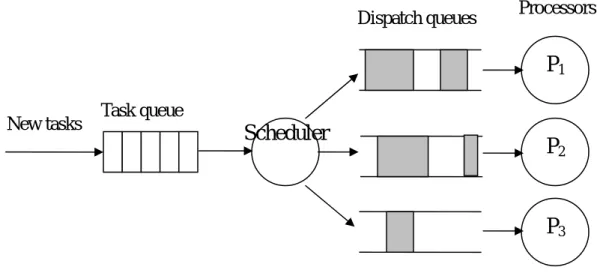
(14) We assume that tasks are aperiodic [2], i.e., the task arrivals are not known a priori. Attributes of a task is unknown until it is generated and enters the system. Periodic task model is a special case of aperiodic task model, so that the algorithm proposed in this thesis is also applied to periodic tasks. We also assume that tasks are independent, i.e., there are no precedence constraints between tasks. Nevertheless, dealing with precedence constraints is equivalent to working with the modified ready times and deadlines [5]. Therefore, the proposed algorithm can also be applied to tasks with precedence constraints among them. There are also no communications between tasks. Finally, tasks are nonpreemptable, i.e., when a task starts execution on a processor, it finishes to its completion.. 2.1.2 Scheduler Model In a dynamic multiprocessor scheduling, all the tasks arrive at a central processor called the scheduler, and are distributed to other processors in the system for execution. Each processor has its own dispatch queue to where scheduled tasks are distributed. The scheduler is running in parallel with other processors, scheduling the newly arriving tasks, and updating the dispatch queues. Fig. 2.1 shows the architecture of the scheduler model. Single scheduler in this model may make a point of failure. The scheduler model may be fault-tolerant by employing modular redundancy technique in which another backup scheduler runs scheduling in parallel with the primary scheduler [2]. Final schedule is chosen from the results of the two schedulers by an acceptance test. A simple acceptance test is to check whether all the tasks in the schedule finish before their deadlines. Due to the assumption of the hard real-time task model, we assume each task is scheduled as soon as possible. That is, the scheduling action of the scheduler may be periodic -5-.

(15) Dispatch queues. Processors. P1 New tasks. Task queue. Scheduler. P2. P3 Fig. 2.1 Scheduler model with a small time quantum or may be starting as a task arrives. Because the scheduler is a dedicated processor, the high frequency of the scheduling would not affect the other general processors.. 2.1.3 Fault Tolerance Model In this thesis, we uses Primary-Backup (PB) model for fault tolerance [3]. In the PB model, each task has two copies, namely, primary copy and backup copy. The backup copy is redundant for the purpose of fault tolerance, and starts execution only when the primary copy fails. Using PB model for fault tolerance, the following necessary conditions are required. (1) Mutually exclusive in space: primary and backup copies must be scheduled on different processors (to tolerate permanent processor faults). (2) Mutually exclusive in time: the start time of a backup copy must be latter than the finish time of its primary copy. This condition also implies two facts. First, the two versions of a task are not parallelizable. Second, the sum of computation times of primary and backup copies should be less than or equal to (di–ri) so that the both copies can be schedulable within this interval.. -6-.

(16) Because backup is the only redundant copy of a task, we assume that each task encounters at most one failure either due to hardware failure or due to software failure. This also implies that there is at most one failure in the system at any instant of time.. 2.2 Related Work Many scheduling problems have been proved to be NP-complete [6], i.e., it was believed that there is no optimal polynomial-time algorithm for them. It was also shown that an algorithm does not exist for optimally scheduling dynamically arriving tasks on a multiprocessor system [7]. These negative results motivated the need for heuristic approaches to solve the scheduling problems. Generally, the heuristic scheduling algorithms try to find a feasible schedule by repeating two steps. The first step is to select one task with the highest priority which is determined by a heuristic function. The heuristic function synthesizes various characteristics of a task to form the priority of scheduling order. The next step is to decide one processor on which the selected task is assigned. The two steps repeat until all tasks in the queue are either scheduled or rejected. In the past decade, many heuristic scheduling algorithms have been proposed to dynamically schedule a set of tasks whose deadlines and computation times are unknown until arriving into the system. For homogenous multiprocessor systems with resource constraint, an algorithm called myopic algorithm was proposed [1]. Initially, myopic sorts all tasks in the nondecreasing order of deadlines. In the task selection step, it checks whether the current partial schedule is strongly feasible. If so, a given heuristic is applied to all tasks in feasibility check window. The task with the lowest heuristic is chosen to extend the current schedule. If the current schedule is not strongly feasible, backtracking is done by discarding the current schedule, and extending the previous schedule by a different task. A partial schedule is said strongly feasible if all the schedules obtained by extending this schedule with -7-.

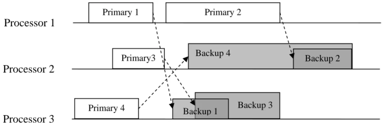
(17) any one task in the feasibility check window are also feasible. Feasibility check window contains the first k tasks in the sorted task queue. In order to reduce the cost of looking ahead, [1] considers only the tasks in the feasibility check window both for strong-feasibility checking and for heuristic calculating. It has been shown that an integrated heuristic, which is a function of the deadline and the earliest start time of a task, outperforms other simple heuristics such as minimum deadline first, minimum computation time first, least laxity first, etc. Myopic is efficient and effective. However, it is limited on homogeneous systems, and does not have the fault-tolerant mechanism which is more and more important for real-time systems. Another issue is about the heuristic function. Myopic sorts all the tasks initially in nondecreasing order of deadlines. When scheduling is in progress, the tasks under consideration are limited in the feasibility check window. Because the size of feasibility check window is small, the order of tasks to be scheduled is close to the order of nondecreasing deadlines. A more realistic heuristic will be defined in the next chapter. In the PB model, backups are redundant if their primaries finish successfully. In order to utilize the redundant time, the concept of overlapping backups is proposed by backup overloading algorithm [3]. Overlapping backups means that more than one backup copy can be overlapped with each other on the same processor. The necessary condition of backup overloading is as follows. If the primary copies of two tasks are scheduled on two different processors, then their backups can be overlapped with each other on a processor. Fig. 2.2 illustrates the backup overloading. Backup1 and Backup3 can be overlapped with each other whose primaries, Primary1 and Primary3, are scheduled on different processors respectively. Similarly, the Backup2 and Backup4 could also be overlapped with each other. Another concept proposed by [3] is backup deallocation. Backup deallocation means the reclamation of resources reserved for backup tasks when the corresponding primaries complete. -8-.

(18) Primary 1. Primary 2. Processor 1 Primary3. Backup 4. Backup 2. Processor 2. Primary 4. Processor 3. Backup 1. Backup 3. Fig. 2.2 Backup overloading successfully. For example, the time interval used by the backups can reutilized if no faults occur. Both of these two techniques help improve acceptance ratio of arriving tasks. For dynamically scheduling tasks with fault tolerance, distance myopic algorithm which is extended from myopic algorithm is proposed in [2]. The main difference between distance myopic and the original myopic algorithm is the construction of task queue. Because PB based fault tolerance is included in this method, all primaries in the task queue are sorted in nondecreasing order of deadlines. Then, the backups are inserted into the task queue at the distance, called distance concept, from their primary copies. The primary always precedes its backup in the task queue. The distance is an input parameter to the scheduling algorithm to determine the relative positions of the two copies of a task in the task queue. The primary and backup of a task are scheduled separately except that the backup could be scheduled until the primary has been scheduled. The other enhancement of distance myopic is flexible backup overloading, which introduces a trade-off between degree of fault tolerance and performance. The flexible overloading scheme permits more than one fault occur at any instant of time by forming the processors into different groups. In each group, there is at most one fault at a time. Putting the primaries and backups in the single task queue is one of main disadvantages in this algorithm. The reason is that a backup may appear in the feasibility check window. -9-.

(19) when its primary is also in the window. The strong feasibility checking is false because the backup is unschedulable. The situation will result in backtracking and eventually rejecting this task. Another disadvantage is that it is difficult to choose the right combination of the two parameters, distance and the size of feasibility check window. With varying situations of system environment, the same values of parameters will not always produce good result. Thus, adjustments to the parameters are needed in different situations. Both of myopic and distance myopic are scheduling real-time tasks on homogeneous multiprocessor systems. Fault-tolerant myopic algorithm (FTMA) [8], which is extended from distance myopic, is used for heterogeneous multiprocessor systems. In addition, the enhancements of FTMA include task queue construction and feasibility check window movement. The main motivation of FTMA is to overcome the disadvantage of single task queue in distance myopic algorithm. FTMA puts primary and backup copies separately in two different task queues, namely primary task queue and backup task queue. Both primaries and backups are sorted in nondecreasing order of deadlines. FTMA selects the task with smaller heuristic value from the first primary and backup in the queues into the check window. The heuristic of a backup is defined as infinite when its primary has not been scheduled. In this way, the two versions of a task will not appear in the window simultaneously. The two-task-queue method also eliminates the need of the distance parameter which is difficult to be chosen. However, the other parameter, size of feasibility check window, is still needed in FTMA. As distance myopic, adjustment to this parameter is still needed in different situations of the system. eFRCD is a static scheduling algorithm on heterogeneous systems [4]. It takes account of the heterogeneities of computation, communication and reliability. Tasks are judiciously allocated to processors so as to reduce the reliability cost, defined to be the product of processor failure rate and task execution time. Like the static algorithms proposed in [19, 30],. - 10 -.

(20) eFRCD schedules all tasks with known attributes a priori. These static algorithms can not be applied to a dynamic system due to their high complexity. The assumption with a priori known attributes is also not realistic for the systems of aperiodic tasks. In the next chapter, we will describe the proposed algorithm which schedules real-time tasks dynamically with fault tolerance on heterogeneous systems without any parameters.. - 11 -.

(21) Chapter 3. Density First with Minimum Non-overlap Scheduling Algorithm We have described the relative background about dynamically scheduling real-time tasks with fault tolerance in the previous chapter. In this chapter, we will propose the density first with minimum non-overlap scheduling algorithm (DNA). As those algorithms introduced in chapter 2, DNA repeats two phases continuously until all tasks in the queue are scheduled or rejected. The first one is the task selection phase followed by the second one, processor assignment phase. In the task selection phase, we define a new heuristic, namely density, to prioritize tasks in the task queue. In the processor assignment phase, the primary copy is scheduled first, and then the next step is backup scheduling. A new strategy, called minimum non-overlap (MNO), is proposed for scheduling backups. In section 3.1, we describe the definition of the density heuristic. In section 3.2, we state the minimum non-overlap strategy for backup scheduling. Finally, the complete algorithm will be presented in section 3.3 followed by the discussion of complexity.. 3.1 A New Heuristic Function In the first phase, a heuristic function is used to decide the priorities of tasks. A task with the highest priority will be selected to be scheduled first. Most scheduling algorithms described in section 2.2 use deadlines and earliest finish times as the integrated heuristic function. This implies that tasks which may or have to finish earlier are given higher priorities. Nevertheless, real-time tasks are not concerned about when to start computation but rather about meeting their deadlines. For example, tasks with earlier deadlines or finish times may have small computation times so that they are still schedulable even with lower scheduling order. On the other hand, tasks with later deadlines or finish times should be given higher - 12 -.

(22) priorities if their computation times are large with respect to their schedulable intervals. The question of whether or not a task Ti could be scheduled by its deadline depends on the relationship between the schedulable intervals of Ti and its computation times on each processor. Thus, we introduce a concept of density as the heuristic function. The time of all schedulable intervals for a task is called schedulable time generally. The density of a task is a ratio of the computation time to the schedulable time. When the computation time needed by Ti is getting closer to its schedulable time, we say that Ti has large density. With large density, it is less flexible to schedule Ti. That is, if Ti does not have higher priority of scheduling order, it may be rejected because the schedulable time is getting less after other tasks are scheduled. Conversely, if the computation time needed by Ti is small with respect to its schedulable time, i.e. small density, Ti may be still schedulable with lower priority. This is because it is easier to find schedulable intervals for tasks with small density than tasks with large density. Before we give the formal definition of density, some terminologies will be defined first. Let Pri and Bki be the primary and backup copies of task Ti respectively, and Proc is the set of all processors in the system. Because of the time exclusion between primary and backup copies of a task, the scheduled start time of Bki must be greater than or equal to the scheduled finish time of Pri. It implies that the deadline of Ti, di, is impossible to be the latest finish time of Pri, and the ready time of Ti, ri, is also impossible to the earliest start time of Bki. In the following, the start or finish time for primary and backup will be redefined. First, Bki is impossible to be scheduled if the interval between the scheduled finish time of Pri and di is less than the minimum computation time of Ti. Thus, Pri must be finished before its latest finish time, LFP(Ti). Actually, LFP(Ti) could be thought of as the deadline of Pri. Finally, we give the following definitions.. - 13 -.

(23) Definition 3.1 The Latest Finish time of Primary (LFP) is defined as: LFP( Ti ) = d i − MIN { cip } , for all p ∈ Pr oc. (1). , where di is the deadline of Ti, and cip is the computation time of Ti on processor p.. In additional to the LFP, Ti has the earliest finish time for its primary.. Definition 3.2 The Earliest Finish time of Primary (EFP) is defined as: EFP( Ti ) = MIN { EST (Pri )p + cip } , for all p ∈ Pr oc. (2). , where EST(Pri)p is the earliest start time of Pri on processor p.. The scheduled start time of Bki could be as early as the earliest finish time of Pri. Thus, we define the earliest start time of backup (ESB) for Ti as: ESB(Ti) = EFP(Ti). (3). ESB(Ti) could also be thought of as the ready time of Bki. With the definitions of LFP and ESB, we could claim that Pri should be scheduled between ri and LFP(Ti), and Bki should be scheduled between ESB(Ti) and di. Neither primary nor backup of a task could be scheduled on the processors without sufficient schedulable time for it. The processor on which the primary or backup could be scheduled may be different. Thus, we define a set of available processors for the primary and backup respectively. Each set contains processors on which the primary (backup) can be scheduled.. Definition 3.3 We define availP(Pri), the set of available processor for Pri, and availP(Bki), the set of available processor for Bki, as follows: (1) availP(Pri) = { processor j }, where there is at least one time slot greater than or - 14 -.

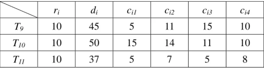
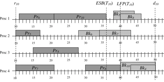
(24) equal to cij between ri and LFP(Ti) on processor j. The slot cannot be overlapped with any scheduled tasks, neither primaries nor backups. (2) availP(Bki) = { processor j }, where there is at least one time slot greater than or equal to cij between ESB(Ti) and di on processor j. The slot can be overlapped with any scheduled backups.. Here, we give an example to demonstrate the above definitions. We assume there are four processors in the system, the current time is 10, and there are three tasks have arrived into the system. Fig. 3.1 shows the current schedule, and Table 3.1 lists the attributes of the tasks in the queue. This example will be used for illustration throughout this chapter. In this example, Pr9 must finish before the time = 40 because the Br9 may be scheduled on processor 3 where T9 has the maximum computation time. Thus, the LFP(T9) is 40. Pr9 could start at time = 17, and has the earliest finish time, 26, on processor 2. This implies Bk9 could start as early as time = 26. Thus the ESB(T9) is 26. Pr9 can be scheduled in the range from the ready time, r9 = 10, to the LFP(T9), 40. On processor 3, there are two time slots, (10, 15) and (28, 40), which are not reserved for any task yet between r9 and LFP(T9). But both of them are less than c93 so that Pr9 could not be scheduled on processor 3. Similarly, Pr9 could not be scheduled on processor 4 because the only unreserved time slot between r9 and LFP(T9), (21, 30), is less than c94. Thus, the set of processors which Pr9 can be scheduled, i.e. availP(Pr9), is {processor 1, processor 2}. Bk9 can be scheduled in the range from the ESB(T9), 26, to the deadline, d9 = 45. Between ESB(T9) and d9, we assume all scheduled backups may be overlapped with Bk9. On processor 1, 2, 3, there are time slots large enough to execute Bk9. However, time slots (26, 30) and (40, 45) are too small to execute Bk9. Thus, the availP(Bk9) is {processor 1, processor 2, processor 3}. As we mentioned early in this section, the density of a task is a ratio of the computation. - 15 -.

(25) d. Table 3.1. Attributes of tasks in the task queue. ri. di. ci1. ci2. ci3. ci4. T9. 10. 45. 5. 11. 15. 10. T10. 10. 50. 15. 14. 11. 10. T11. 10. 37. 5. 7. 5. 8. Bk5. Pr6. Proc 1 10. 25. 20. 15. 30. Pr5. Proc 2 10. 35. Bk6 15. 20. Bk8. 40. 45. 50. Bk7. 25. 30. 35. 40. 45. 50. 25. 30. 35. 40. 45. 50. Pr4. Proc 3 10. 15. 20. Pr7. Proc 4 10. Pr8. 15. 20. 25. 30. 35. Bk4 40. 45. 50. Fig. 3.1. The schedule at time = 10. Dark shading areas depict scheduled primaries. Grey shading areas depict scheduled backups. time to its schedulable time. First, because of the two copies of a task, the computation time needed by Ti includes the time for Pri and Bki. Actually, we define the time needed by primary and backup as the average computation time on those processors in the availP(Pri) and availP(Bki) respectively.. Definition 3.5 For task Ti, we define Pr_mean, the average computation time of Pri on availP(Pri), and Bk_mean, the average computation time of Bki on availP(Bki) as follows:. Pr_ mean( Ti ) = Bk _ mean( Ti ) =. ∑c. ip p∈availP(Pri ). ∑c. ip p∈availP( Bki ). availP(Pri ) availP( Bk i ). (4). (5). , where availP(Pri ) and availP( Bki ) are the number of processor in availP(Pri) and - 16 -.

(26) availP(Bki) respectively.. Next, the schedulable time for Ti is the sum of time slots which are schedulable for Pri or Bki. A time slot, represented as (start, end), which is schedulable for Pri on processor p is defined as prslotip. prslotip must satisfies the following conditions: (1) start ≥ ri , (2) end ≤ LFP( Ti ) , (3) end − start ≥ cip , (4) prslotip cannot be overlapped with any scheduled primaries or backups on processor p. A time slot which is schedulable for Bki on processor p is defined as bkslotip. Similarly, bkslotip must satisfy: (1) start ≥ ESB( Ti ) , (2) end ≤ d i , (3) end − start ≥ cip , (4) bkslotip cannot be overlapped with scheduled primaries on processor p. For Ti, the total schedulable time is the sum of all prslotip and bkslotip.. Definition 3.6 The Sum of Schedulable Time of Ti, named SST, is defined as:. SST ( Ti ) =. ∑ prslot. p∈availP(Pri ). ip. +. ∑ bkslot. p∈availP( Bki ). ip. ,. (6). After introducing the above definitions, we could define the new heuristic function, named density function, as follows.. Definition 3.4 For each task Ti in the task queue, we define the density heuristic function as:. density( Ti ) =. Pr_ mean( Ti ) + Bk _ mean( Ti ) SST ( Ti ). (7). The density of a task indicates the tightness of the interval between the ready time and the deadline with respect to its computation time. The highest density means that it is least flexible to schedule a task. On the other hand, low density means that it is easy to find. - 17 -.

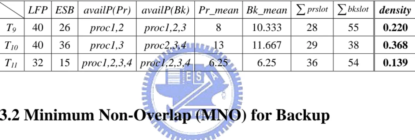
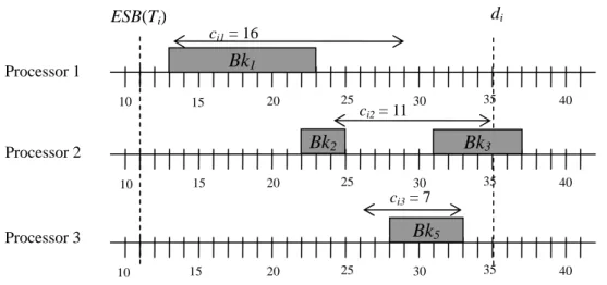
(27) schedulable intervals for primary and backup. Thus, we will select the task with the maximum density in task selection phase. It is to be noted that the density is defined for a task Ti, rather than Pri or Bki separately. The reason is that Ti will be rejected if either Pri or Bki fails to be scheduled. Getting less flexible to schedule either Pri or Bki implies that it is also inflexible to schedule Ti. Table 3.2 gives an example of density calculation for the tasks in table 3.1. T10 are given the highest priority even though both of the EFT(Pr10) and d10 are larger than the other tasks.. Table 3.2. Density calculation for T9, T10, T11 in Table 3.1. LFP ESB availP(Pr) availP(Bk) Pr_mean Bk_mean ∑ prslot ∑ bkslot. density. T9. 40. 26. proc1,2. proc1,2,3. 8. 10.333. 28. 55. 0.220. T10. 40. 36. proc1,3. proc2,3,4. 13. 11.667. 29. 38. 0.368. T11. 32. 15. 6.25. 6.25. 36. 54. 0.139. proc1,2,3,4 proc1,2,3,4. 3.2 Minimum Non-Overlap (MNO) for Backup After selecting the task with the maximum density in the first phase, DNA starts to schedule the primary and backup in the second phase. As many scheduling algorithms for heterogeneous systems, we will schedules the primary on the processor where it could finish as early as possible. In the next step for scheduling backup, most algorithms like those described in section 2.2.1 also assign a backup to a processor according to the earliest finish time. The processor time reserved for backups, however, is redundant and will be deallocated if their primaries finish successfully. If the processor time reserved for backups could be minimized, there is more schedulable time for other new tasks. An intuitive method for this idea is to overlap backups as much as possible. It works for homogeneous systems, but doesn’t work for heterogeneous systems. This is because the computation time of a task varies from processor to processor in heterogeneous systems. For a task Ti, having the maximum - 18 -.

(28) di. ESB(Ti) ci1 = 16. Bk1. Processor 1 10. 15. 25. 20. ci2 = 11. Bk2. Processor 2 10. 15. 40. Bk3 25. 20. 35. 30. 30. 35. 40. 35. 40. ci3 = 7. Bk5. Processor 3 10. 15. 25. 20. 30. Fig. 3.2. The maximum overlapped time of Bki is 10 on processor 1. The minimum non-overlapped time of Bki is 2 on processor 3. overlapped time on processor p does not necessarily mean that Ti also has the minimum non-overlapped time on processor p. The non-overlapped time is actually the extra processor time being reserved for Bki. For example, in Fig. 3.2, lines with double arrows represent the computation time and the possible schedule of Bki where it has the minimum non-overlapped time on that processor. It is shown that Bki has the maximum overlapped time on processor 1, however 6 extra time units, i.e. interval (23, 29), are required. Similarly, 6 extra time units will be required for processor 2. Bki has the minimum non-overlapped time, 2, on processor 3 means that only 2 extra time units will be reserved for it. Thus, we will intend to minimize the extra time being reserved for backups, i.e. non-overlapped time. That is, a backup will be scheduled on the processor where it has the minimum non-overlapped time. We give the definition of minimum non-overlap of a backup as follows.. Definition 3.7 The Minimum Non_Overlap (MNO) of Bki is defined as: MNO( Bk i ) = MIN { cip − MAXoverlap ip } , for each p ∈ Pr oc. , where Maxoverlapip is the maximum overlapped time of Bki on processor p.. - 19 -. (8).

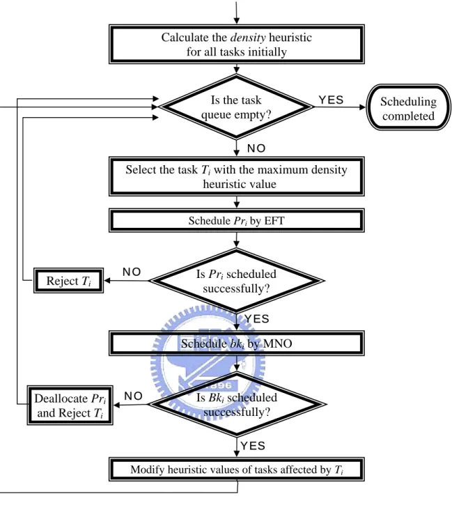
(29) r10 Pr6. Proc 1 10. 15. 10. Bk5. Pr10 25. 20. Pr5. Proc 2. d10. ESB(T10) LFP(T10). 30. 35. 20. 40. 45. 50. Bk7. Bk6 15. Bk8. 25. 30. 35. 40. 45. 50. 25. 30. 35. 40. 45. 50. Pr4. Proc 3 10. 15. 20. Pr7. Proc 4 10. 15. Pr8 20. 25. 30. 35. Bk10 40. Bk4 45. 50. Fig. 3.3. MNO(Bk10) is 3 on processor 4.. On each processor, we try to find the maximum overlapped time for Bki in order to minimize the non-overlapped time. Finally, Bki will be scheduled on the processor where MNO(Bki) is obtained. For the example in section 3.1, T10 has the maximum density and Pr10 is scheduled on processor 1 by its EFT shown in Fig.3.3. The schedule of Bk10 on processor 2 is exactly the interval (ESB(T10), d10), and the non-overlapped times is 7. On processor 3, there is no any backup to be overlapped with so that the non-overlapped time equals the c10,3, 11. On processor 4, Bk4 could be overlapped with Bk10 completely, and the non-overlapped time is only 3. Obviously, if Bk10 is scheduled on processor 4, the extra processor time reserved for it is only 3. Thus, MNO(Bk10) is 3 and Bk10 will be scheduled on processor 4 even though the maximum overlapped time is on processor 2, and the earliest finish time is on processor 3.. 3.3 The DNA Algorithm After introducing the concepts of density and MNO, the complete algorithm of DNA is described in this section. Fig. 3.4 shows the flow of our DNA algorithm. Similar to most - 20 -.

(30) Calculate the density heuristic for all tasks initially. Is the task queue empty?. YES. Scheduling completed. NO. Select the task Ti with the maximum density heuristic value Schedule Pri by EFT. Reject Ti. NO. Is Pri scheduled successfully? YES. Schedule bki by MNO. Deallocate Pri and Reject Ti. NO. Is Bki scheduled successfully? YES. Modify heuristic values of tasks affected by Ti. Fig. 3.4 Flow chart of DNA algorithm heuristic scheduling algorithms, the steps involved in DNA divided into two phases. The two phases repeats continuously until the task queue is empty. The first phase is to select the task with the maximum density as the candidate to be scheduled. In the second phase, we try to schedule the primary copy of the selected task first. If successfully, the next step is trying to schedule the backup copy. A task is said to be scheduled successfully only if both copies are scheduled successfully. Conversely, the selected task will be rejected if either the primary or - 21 -.

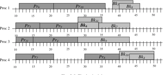
(31) 10. 15. Bk5. Pr10. Pr6. Proc 1. 25. 20. 35. 30. Bk8. 40. 45. 50. 40. 45. 50. 40. 45. 50. Bk11 Pr5. Proc 2. Pr9 15. 10. 10. 25. 20. Pr11. Proc 3. Bk6 30. Pr4 15. 20. 10. 15. 35. Bk9 25. 30. Pr7. Proc 4. Bk7. 35. Pr8 20. 25. 30. 35. Bk10 40. Bk4 45. 50. Fig. 3.5. Final schedule. the backup fails to be scheduled. For the previous example, after T10 is scheduled successfully, we recalculate the density of the remaining tasks, T9, T11. The next one to be scheduled is T9 with density = 0.395, and T11 is the last one. The final schedule is shown in Fig. 3.5. It is to be noted that after a task with the maximum density has been selected, we schedule the primary first, and then, schedule the backup immediately. This is different from many fault-tolerant scheduling algorithms, such as distance myopic and FTMA which schedule primaries and their backups as distinct tasks [2, 8]. The reason is that the density heuristic function determines the priorities among all original tasks, neither primaries nor backups. The advantage is that there is no need for task queue construction any more. That is, the distance parameter in distance myopic algorithm and the separated task queues in FTMA are eliminated. It is also to be noted that we have no checking strong feasibility and backtracking which are used in distance myopic and FTMA [2, 8]. The purpose of checking strong feasibility is for looking ahead. Although the feasibility check window decreases the number of tasks to be checked, the overhead of checking each task exists at each selection phase. We just apply the density heuristic function to all the remaining tasks in the task queue. Because of the assumption of dynamic systems and scheduler model defined in chapter 2, the number of - 22 -.

(32) tasks in the task queue should not become so large while the scheduler starts scheduling. Thus, the overhead of the task selection shall not be very heavy. We need no backtracking in our algorithm. If either primary or backup fails to be scheduled, this task is just rejected. Both steps of checking and backtracking will increase the running time of algorithms in realistic systems. Thus, we neither check the strong feasibility of the current partial schedule, nor backtrack to the previous schedule if the selected task is not schedulable. It is just scheduling all the tasks one by one. Because we take all tasks into consideration in the task selection phase, the complexity of worst case is O(n2). n is the number of tasks to be scheduled. The complexity is higher than that of FTMA and distance myopic, O(n). Nevertheless, n shall not be very large in the assumption of our scheduler model. In addition, a trick could also reduce the run time cost. The density heuristic function is applied to all tasks only before the repeat of the two scheduling phases. After a task is scheduled successfully, the heuristic function may not be applied to all the remaining tasks in the next task selection phase. Only those tasks, which have schedulable time slots overlapped with the just scheduled primary or backup, will be given the recalculated density.. In the next chapter, we will evaluate our DNA algorithm using simulation. The simulation result of DNA will compare with distance myopic and FTMA.. - 23 -.

(33) Chapter 4. Simulation and Performance Evaluations In this chapter, we will evaluate the performance of density first with minimum non-overlap scheduling algorithm (DNA) through simulation. In section 4.1, we will describe the architecture of the simulator and some simulation parameters. Next, we will give the performance evaluations in section 4.2.. 4.1 Simulation Construction Because DNA is a dynamic scheduling algorithm, we will construct a dynamic simulation instead of a static simulation. The flow of dynamic simulation is divided into two parts. The first one is the task generator which generates a set of real-time tasks as the input of the second part, simulator. The simulator simulates the events in the systems and the actions of the scheduler. In the following, we will describe how to construct these two parts.. 4.1.1 Task Generator The task generator generates a set of real-time tasks in the non-decreasing order of arriving times. Each task has the attributes as described in section 2.1.1. The parameters which affect these attributes in the task generation are summarized in Table 4.1. In the following, we will describe how to decide the attributes of a task. The computation time of a task varies from processor to processor, and is bounded by the minimum and maximum computation time, MIN_C and MAX_C. The heterogeneity variable, which is chosen uniformly between 0 and 1, represents the heterogeneity of computation times of a task. It determines the range of possible computation times for a task. Thus,. - 24 -.

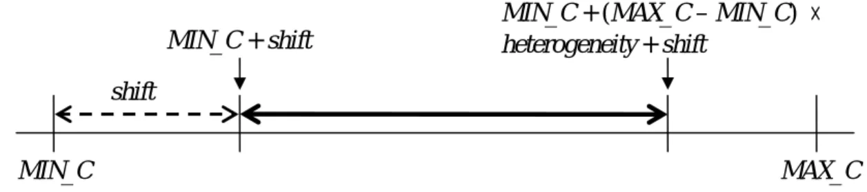
(34) ddddddd. Table 4.1. Parameters for task generator. parameter. explanation. range of possible values. MIN_C. minimum computation time. 10. MAX_C. maximum computation time. 80. λ. task arrival rate. R. laxity. P. number of processors. [3, 10] (integer). BurstP. probability of a burst. λ 100. [0.3, 0.9] (real) [2, 7] (real). MAX_Burst. maximum task number for a burst. 10. MIN_Burst. minimum task number for a burst. 30. computation times of a task are chosen uniformly in the range of MIN_C and MIN_C + (MAX_C – MIN_C) × heterogeneity. The lower bound, however, is not always MIN_C, so the range will be shifted by the variable shift. Because the upper bound cannot larger than MAX_C, the shift is chosen uniformly between 0 and MAX_C – (MAX_C – MIN_C) × heterogeneity. Finally, computation times of a task are chosen uniformly between (MIN_C + shift) and (MIN_C + ((MAX_C – MIN_C) × heterogeneity) + shift). Fig. 4.1 shows the range of computation time. The arrival times of tasks depend on the interarrival time between each task. The interarrival time is exponentially distributed with mean [2]: 1 MIN _ C + MAX _ C × λ×P 2. , where λ is the task arrival rate, and P is the number of processors. We also assume there is a possibility of bursts of tasks. We define the mean of interarrival time for bursting is 1 MIN _ C × λ×P 10. The probability of burst, BurstP, varies with λ and is defined as λ 100 . When a burst. - 25 -.

(35) MIN_C + (MAX_C – MIN_C) × heterogeneity + shift. MIN_C + shift shift MIN_C. MAX_C. Fig. 4.1. The solid line with double arrows is the range of possible computation time.. (ai + max cip + second max cip). ai. max cip. second max cip. max cip. max cip. (ai + 3 × max cip). max cip. Fig. 4.2. di is chosen uniformly in the range of the solid line with double arrows when laxity = 3.. happens, there are at least MIN_Burst tasks and at most MAX_Burst tasks arriving at the systems in a very short interval. Because both copies may be scheduled with the first two maximum computation times, the deadline of a task must be late enough to satisfy this possible scheduling. Thus, the deadline of a task Ti is uniformly chosen between (ai + max cip + second max cip) and (ai + R × max cip). The laxity parameter, R, indicates the tightness of the deadline, and is at least 2. Fig. 4.2 depicts the lower and upper bound of deadline when laxity = 3.. 4.1.2 Simulator Our evaluation was done by implementing a discrete-event dynamic simulator [17]. The dynamic simulator simulates all events which may happen in a realistic system. The possible events include the arrival, start and completion of a task, start of the scheduling, and backup - 26 -.

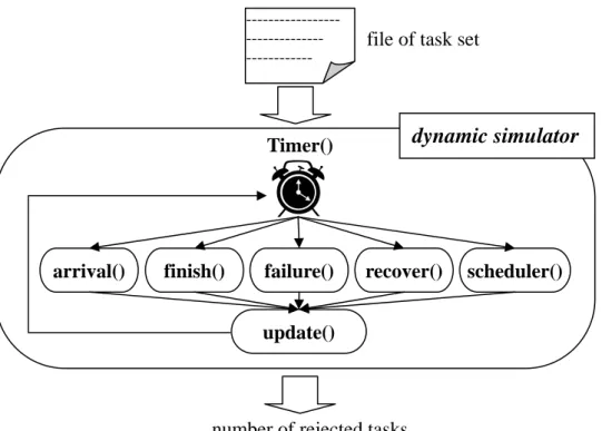
(36) -----------------------------------------. file of task set. dynamic simulator. Timer(). arrival(). finish(). failure(). recover(). scheduler(). update(). number of rejected tasks Fig. 4.3. Flow of the dynamic simulator. deallocation as well as occurrence of faults. Fig. 4.3 depicts the flow of the dynamic simulator. After reading the task set generated by the task generator, the Timer function decides the time of next event, and calls the corresponding operation. After dealing with the events, the update function updates the status of the system. The flow will repeat until all tasks in the set have arrived into the system and completed or been rejected. At the end time, the simulator terminates and reports the number of rejected tasks. For reality, we simulate the failure events. The failures may be due to hardware fault or software fault [2]. Because the backup copy is the only one redundancy, we assume that each task encounters at most one failure. That is, the backup always succeeds if its primary fails. A software fault will terminate the task immediately. The hardware faults are the faults happened to processors. All tasks on the failed processor will be terminated and deallocated, whatever they are running or ready to run. The hardware faults could be transient or permanent. If a transient fault happens, the failed processor will be available again in some recovery time. The recovery time is distributed normally between 0 and MAX_Recovery. If a - 27 -.

(37) d. Table 4.2. Parameters for fault probability. parameter FaultP Soft_FP Hard_FP. explanation probability that a primary fails probability that a primary fails due to software fault probability that a primary fails due to hardware fault. PermHard_FP. probability that a hardware fault is permanent. MAX_Recovery. maximum recovery time after a transient hardware fault happened. range of possible value [0, 0.5] (real) 0.2 0.8 0.000001 50. permanent fault happens, the failed processor would never be available to the end of simulation. We define the relative probabilities and parameters for failure events in Table 4.2.. 4.2 Performance Evaluations In this section, we will evaluate the performance of the DNA algorithm by comparison with FTMA and a modified distance myopic algorithm for heterogeneous systems, called HDMA. HDMA is proposed in [8]. The total number of tasks arrived into the system is 20,000. For each set of parameters of the task generator, 20 task sets are generated as the inputs of the three algorithms. We take the average of the 20 rejection number as the final result. HDMA needs two parameters, size of feasibility check window (K) and distance, and FTMA needs one, i.e. K. Because the better results depend on the combination of these parameters, we will run HDMA with various combinations of K and distance, and run FTMA with various K for each task set. We will choose the best result among the various combinations of parameters as the final result of HDMA and FTMA for each task set. Next, we define the metric for the performance evaluations. The objective of any dynamic real-time scheduling algorithm is to improve the guarantee ratio. The guarantee ratio is defined as the percentage of tasks whose deadlines are met [1]. The formal definition is - 28 -.

(38) given below: Guarantee Ratio =. number of tasks whose deadlines are met × 100% total number of tasks arrived in the system. (9). In the next subsections, we will evaluate the performance of DNA and the other algorithms with four simulation parameters. These parameters are task arrival rate ( λ ), laxity (R), processor number (P), and fault probability (FaultP).. 4.2.1 The Effect of Task Load The task arrival rate (λ) has been varied in Fig. 4.4. The size of feasibility check window, K, ranges from 6 to 10 for FTMA. For HDMA, K ranges from 3 to 8 and the distance ranges from 5 to 8. Higher λ means lower interarrival time and, thus, higher task load. As task load increases, the guarantee ratio decreases for all algorithms. Obviously, HDMA has poor performance because of the single task queue for primaries and backups. Appearances of a primary and its backup in the feasibility check window results in continuously backtracking and rejecting eventually. FTMA overcomes this disadvantage and has almost the same guarantee ratio as DNA with lower arrival rate. When the task load is getting higher, DNA rejects fewer tasks than that of FTMA. This implies that the density heuristic function selects more appropriate tasks to be scheduled when more and more tasks arrived at the system in an interval.. 4.2.2 The Effect of Laxity The effect of task laxity (R) is depicted in Fig. 4.5. The size of feasibility check window, K, ranges from 6 to 10 for FTMA. For HDMA, K ranges from 3 to 8 and the distance ranges from 5 to 8. As the laxity increases, the guarantee ration also increases for all algorithms. We. - 29 -.

(39) DNA. 100%. FTMA HDNA. Guarantee ratio. 95% 90% 85% 80% 75% 70% 65% 60% 0.3. d. 0.35. 0.4. 0.45. 0.5. 0.55. 0.6. 0.65. 0.7. Task arrival rate (λ). 0.75. 0.8. 0.85. 0.9. Fig 4.4. Effect of task load. (R = 3, P = 8, FaultP = 0.2). Guarantee ratio. 90%. DNA. FTMA. HDMA. 85%. 80%. 75%. 70% 2. 3. 4. 5. 6. Laxity (R). 7. 8. 9. 10. Fig. 4.5. Effect of laxity. ( λ = 0.7, P = 8, FaultP = 0.2). can find that the difference of the performance between DNA and the other algorithms is the largest with the smallest laxity, and is getting closed when laxity is bigger. This is because the density heuristic function considers the relationship between computation time and schedulable interval rather than the deadline. It will give the highest priority to the least flexible task whatever the laxity is. Instead, in the other algorithms, the deadline is synthesized as part of the integrated heuristic function directly. In the situation of low laxity, - 30 -.

(40) 95%. DNA. FTMA. HDMA. Guarantee ratio. 90% 85% 80% 75% 70% 65% 60% 55% 3. dd. 4. 5. 6. 7. 8. Number of Processors (P). 9. 10. Fig 4.6. Effect of the number of processor. ( λ = 0.7, R = 3, FaultP = 0.2). the integrated heuristic function may not select the appropriate task to be scheduled first.. 4.2.3 The Effect of the Number of Processor The effect of varying the number of processors (P) is given in Fig.4.6. The size of feasibility check window, K, ranges from 1 to 12 for FTMA. For HDMA, K ranges from 3 to P and the distance ranges from P/2 to P. To increase the number of processor will increases the guarantee ratio for all algorithms. When more processors are available, the difference in guarantee ratio between DNA and the other algorithms is getting large. This is because there are more opportunities for a backup to be overlapped. The DNA could benefit from this situation since the MNO strategy has more opportunities to find less non-overlapped time.. 4.2.4 The Effect of Fault Probability In Fig. 4.7-4.9, the probability that a primary copy encounters a failure (FaultP) is varied with three parameters, λ, R, and P. We compare DNA only with FTMA for simplicity since - 31 -.

(41) DNA (λ= 0.4) DNA (λ= 0.6). FTMA (λ= 0.4) FTMA (λ= 0.6). DNA (λ= 0.8). FTMA (λ= 0.8). DNA (R = 2) DNA (R = 6). FTMA (R = 2) FTMA (R = 6). DNA (R = 10). FTMA (R = 10). 90%. 100%. Guarantee ratio. Guarantee ratio. 95%. 90%. 85%. 85%. 80%. 80%. 75%. 70%. 75% 0 0.1 0.2 0.3 0.4 0.5 Primary Fault Probability (FaultP). 0 0.1 0.2 0.3 0.4 0.5 Primary Fault Probability (FaultP). Fig. 4.7. Effect of fault probability with various task loads. (R = 3, P = 8). Fig. 4.8. Effect of fault probability with various laxity. (λ= 0.7, P = 8). DNA (P = 5). FTMA (P= 5). DNA (P = 8) DNA (P = 10). FTMA (P = 8) FTMA (P = 10). 95%. Guarantee ratio. 90%. 85%. 80%. 75%. 70% 0 0.1 0.2 0.3 0.4 0.5 Primary Fault Probability (FaultP). Fig. 4.9. Effect of fault probability with various number of processor. (λ= 0.7, R = 3) the HDMA does not outperform the other algorithms in the previous simulation results. As FaultP increases, the guarantee ratio decreases in any situation. When FautP = 0, there is no - 32 -.

(42) fault in the system, which means that every backup will be deallocated and all the time reserved for backups will be reutilized. When the fault probability increases, more backup copies are active to be executed so that it cannot be overlapped with any backups of new tasks. Thus, there is the most time which can be reutilized as fault probability equals 0, and less and less as fault probability increases. In additional, the results of different degree of parameters,. λ, R, P, are the same as the simulation results shown in the above subsections. These figures also show that DNA has higher guarantee ratio than FTMA in any degree of parameters as the fault probability increases.. By the simulation, we have verified the performance of the DNA algorithm. We find that the density heuristic function selects more appropriate tasks to be scheduled, even when the task load is heavy or the deadlines are tight. We also find that the MNO strategy saves more processor time than EFT or overlap as mush as possible for new arriving tasks. Furthermore, without any input parameter, DNA still has better guarantee ratio than that of HDMA or FTMA.. - 33 -.

(43) Chapter 5. Conclusion and Future Work In this thesis, we have proposed an algorithm, named DNA, for dynamically scheduling arriving real-time tasks with PB-based fault-tolerant requirement in a heterogeneous multiprocessor system. Through the dynamic simulation, we have evaluated the performance of the proposed algorithm compared with distance myopic algorithm and FTMA. Finally, in this chapter, we make conclusions and describe some future work about our research.. 5.1 Conclusion The integrated heuristic function proposed in [1] is used by most algorithms which dynamically schedule arriving real-time tasks. The integrated heuristic function emphasizes whether a task could be executed earlier. Nevertheless, real-time tasks are not concerned about when to start computation but rather about meeting deadlines. We propose a new heuristic function, named density, which indicates the tightness of a task. The density function takes account of the schedulable time and the computation time. A task with the highest density means that it is the least flexible to be scheduled so that it will be selected first for scheduling. The simulation results show that the density function selects more appropriate tasks even with a heavy task load. The MNO strategy for backup scheduling will minimize the processor time reserved for backups. This will also increase the schedulable time for new tasks. Obviously, MNO saves more time than overlapping as much as possible on heterogeneous multiprocessor. Moreover, though simulation, we can find that MNO save more and more time than the EFT strategy when the processor number increases. Finally, DNA does not need to be adjudged by any input parameters, unlike the distance myopic and FTMA. Though the simulation, DNA gets better results than those of distance - 34 -.

(44) myopic and FTMA which are the best among any combination of needed parameters. This means DNA is more general and suitable for any environment.. 5.2 Future Work In additional to the research results we have proposed, there are some issues in the future work. First, the assumption of our scheduler model is a dedicated processor for scheduling, and the scheduling overhead is ignored. However, the scheduler may have a lot of idle time if the task load is low. This is not economic for a cost-sensitive system. The scheduler may be used for computation while it is idle as well as scheduling tasks. In this way, the scheduling overhead needs to be taken into account for those tasks scheduled on the scheduler. How to define and quantify the scheduling overhead is not trivial and becomes the next extension of this thesis. Second, most algorithms assume deadlines of tasks are fixed after they are released, i.e. deadlines do not vary with time. For some real-time applications whose high-level requirements may change with time, the model of variable deadlines is required. [26] has proposed a new workload model, called the state-dependent deadline model, for this kind of applications. How to modify the density function in our algorithm for the variable deadline model is another future extension of our research.. - 35 -.

(45) Bibliographies [1] Krithi Ramamritham, John A. Stankovic, and Perng-fei Shiah, "Efficient Scheduling Algorithms for Real-time Multiprocessor Systems," IEEE Trans. on Parallel and Distributed Systems, vol. 1, no. 2, pp. 184-194, Apr. 1990. [2] G. Manimaran and C. Siva Ram Murthy, "A Fault-tolerant Dynamic Scheduling Algorithm for Multiprocessor Real-time Systems and Its Analysis," IEEE Trans. on Parallel and Distributed Systems, vol. 9, no. 11, pp. 1137-1152, Nov. 1998. [3] Sunondo Ghosh, Rami Melhem, and Daniel Mosse, "Fault-tolerance Through Scheduling of Aperiodic Tasks in Hard Real-time Multiprocessor Systems," IEEE Trans. on Parallel and Distributed Systems, vol. 8, no. 3, pp. 272-284, Mar. 1997. [4] Xiao Qin, Hong Jiang, and David R. Swanson, "An Efficient Fault-tolerant Scheduling Algorithm for Real-time Tasks with Precedence Constraints in Heterogeneous Systems," Proc. International Conference on Parallel Processing, pp. 360-368, 2002. [5] J.W.S. Liu, W.K. Shih, K.J. Lin, R. Bettati, and J.Y. Chung, “Imprecise Computations,” Proc. IEEE, vol. 82, no. 1, pp. 83-94, Jan. 1994. [6] M.R. Garey and D.S. Johnson, Computers and Intractability: A Guide to the Theory of NP-Completeness. San Francisco: W.H. Freeman, 1979. [7] M.L. Dertouzos and A.K. Mok, “Multiprocessor On-Line Scheduling of Hard Real-Time Tasks,” IEEE Trans. Software Eng., vol. 15, no. 12, pp. 1,497-1,506, Dec. 1989. [8] Yi-Hsuan Lee and Cheng Chen, “Effective Fault-tolerant Scheduling Algorithm for Real-time Tasks on Heterogeneous Systems,” Proc. National Computer Symposium, pp. 302, 2003. [9] C.M. Krishna and K.G. Shin, Real-Time Systems, McGraw-Hill Int’l, 1997. [10] Y. Oh and S. Son, “Multiprocessor support for Real-Time Fault-Tolerant Scheduling,”. - 36 -.

(46) Proc. IEEE Workshop Architectural Aspects of Real-Time Systems, pp. 76-80, Dec. 1991. [11] T. –Y. Yen and W. Wolf, Hardware-Software Co-Synthesis of Distributed Embedded Systems, Kluwer Academic Publishers, 1996. [12] A.K. Mok, Fundamental Design Problems of Distributed Systems for Hard Real-Time Environments, Doctoral Thesis TR-297, MIT, Laboratory for Computer Science, Cambridge, Mass., 1983. [13] Chi-Sheng Shih and Jane W.S. Liu, “State-Dependent Deadline Scheduling,” Proc. IEEE Real-Time Systems Symposium, pp. 3-14, Dec. 2002. [14] K. Ramamritham and J.A. Stankovic, “Scheduling Algorithms and Operating Systems Support for Real-Time Systems,” Proc. IEEE, vol. 82, no. 1, pp. 55-67, Jan. 1994. [15] L.V. Mancini, “Modular Redundancy in a Message Passing System,” IEEE Trans. Software Eng., vol. 12, no. 1, pp. 79-86, Jan. 1986. [16] K.G. Shin and P. Ramanathan, “Real-Time Computing: A New Discipline of Computer Science and Engineering,” Proc. IEEE, vol. 82, no. 1, pp. 6-24, Jan. 1994. [17] Averill Law and W. David Kelton, Simulation Modeling and Analysis, McGraw-Hill, 1999. [18] Babak Hamidzadeh and Yacine Atif, “Dynamic Scheduling of Real-time Tasks, by Assignment”, IEEE Concurrency, vol. 6, issue 4, pp. 14-25, Oct. – Dec. 1998. [19] T. Tsuchiya, Y. Kakuda, and T. Kikuno, “A new Fault-Tolerant Scheduling Technique for Real-Time Multiprocessor Systems,” Proc. 2nd International Workshop on Real-Time Computing and Applications, pp. 197-202, Oct. 1995. [20] R. Al-Omari, Arun K. Somani, and G. Manimaran, “A New Fault-tolerant Technique for Improving Schedulability in Multiprocessor Real-time Systems”, Proc. 15th International Parallel and Distributed Processing Symposium, pp. 32-39, Apr. 2001. [21] R. Al-Omari, G. Manimaran, and Arun K. Somani, “An Efficient Backup-overloading for. - 37 -.

(47) Fault-tolerant Scheduling of Real-time Tasks”, Proc. IEEE Workshop on Fault-tolerant Parallel and Distributed Systems, pp. 1291-1295, 2000. [22] A. Girault, H. Kalla, M. Sighireanu, and Y. Sorel, “An Algorithm for Automatically Obtaining Distributed and Fault-Tolerant Static Schedules,” Proc. International Conference on Dependable Systems and Networks, pp. 159-168. June 2003. [23] Y. Sorel, “Massively Parallel Computing Systems with Real Time Constraints ‘The Algorithm Architecture Adequation’ Methodology,” Proc. Massively Parallel Computing Systems, pp. 44-53, May 1994. [24] A. Girault, C. Lavarenne, M. Sighireanu, and Y. Sorel, “Fault-Tolerant Static Scheduling for Real-Time Distributed Embedded Systems,” Proc. 21st International Conference on Distributed Computing Systems, pp. 695-698, Apr. 2001. [25] Y. Oh and S. H. Son, “Scheduling Real-Time Tasks for Dependability,” J. Operational Research Society, vol. 48, no. 6, pp. 629-639, Jun. 1997. [26] Chi-Sheng Shih, Lui Sha, and Jane W.S. Liu, “Scheduling Tasks with Variable Deadlines,” Proc. 7th Real-Time Technology and Applications Symposium, pp. 120-122, 2001. [27] G. Manimaran, C. Siva Ram Murthy, M. Vijay, and K. Ramamritham, “New Algorithms for Resource Reclaiming form Precedence Constrained Tasks in Multiprocessor Real-Time Systems,” J. Parallel and Distributed Computing, vol. 44, no. 2, pp. 123-132, Aug. 1997. [28] I. Ekmecic, I. Tartalja, and V. Milutinovic, “A Survey of Heterogeneous Computing: Concepts and Systemds,” Proc. IEEE, vol. 84, pp. 1127-1144, Aug. 1996. [29] B.W. Johnson, Design and Analysis of Fault Tolerant Digital Systems, Addison Wesley, 1989. [30] C.M. Krishna and K.G. Shin, “On Scheduling Tasks With Quick Recovery From. - 38 -.

(48) Failure,” IEEE Trans. Computers, vol. 35, no. 5, pp. 448-455, 1986.. - 39 -.

(49)