在超長指令字的數位訊號處理器下的指令排程以降低能量消耗為目的

全文

(1)國立交通大學資訊工程學系. 碩士論文. 在超長指令字的數位訊號處理器下的指令排程以降低能量消耗為目的. Instruction Level Scheduling for Low-Power on VLIW DSP. 研究生 : 楊偉帆指導教授 : 陳正教授. 中華民國九十四年六月.

(2) 在超長指令字的數位訊號處理器下的指令排程以降低能量消耗為目的 Instruction Level Scheduling for Low-Power on VLIW DSP 研究生 : 楊偉帆. Student : Wei-Fan Yang. 指導教授 : 陳正教授. Advisor : Prof. Cheng Chen. 國立交通大學資訊工程學系碩士論文 A Thesis Submitted to Institute of Computer Science and Information Engineering College of Electrical Engineering and Computer Science National Chiao Tung University in partial Fulfillment of the Requirements for the Degree of Master in Computer Science and Information Engineering June 2005 Hsinchu, Taiwan, Republic of China. 中華民國九十四年六月 -1-.

(3) 在超長指令字架構下的數位訊號處理器作指令排程以降低能量消耗為目的研究生 : 楊偉帆. 指導教授 : 陳正教授. 國立交通大學資訊工程學系碩士班. 摘要個人攜帶式產品在現代生活中已經越來越普及。例如手機、數位照相機、PDA 等等。他們大都是靠充電電池運作，所以如何降低他們的電力消耗以延長他們的使用時間變成一個很重要的議題。而在處理器消耗能量的比例方面，指令的匯流排因為變化很頻繁，所以它佔了很大的比例。其中 switching activities 是影響指令匯流排能量消耗的一個很重要的因素。我們在本篇論文中針對降低 switching activities 提出ㄧ個方法 Greedy Switching Activities Scheduling (GSAS)。GSAS 包含了兩個階段，第一個階段是針對指令做排程並以降低 switching activities 為目的。根據實驗結果 GSAS 比 MSAS 更省能量消耗。第二階段是針對第一階段排出的 schedule 做 registers re-assign 的動作，目的也是爲了降低 switching activities，而根據實驗結果可以發現第二階段可以更近ㄧ步的結省電力的消耗。. i.

(4) Instruction Level Scheduling for Low-Power on VLIW DSP Student : Wei-Fan Yang. Advisor : Prof. Cheng Chen. Institute of Computer Science and Information Engineering National Chiao Tung University. Abstract Portable devices become so popular nowadays. How to reduce the power consumption in these portable devices, such as digital camera, cellular phone, PDA, etc., becomes a more and more important issue. Switching activities is one of the most important factors in power dissipation. In this thesis, we focus on reducing the power consumption of application on VLIW architectures by reducing switching activities on the instruction bus. An algorithm, Greedy Switching Activities Scheduling (GSAS) is proposed. The algorithm contains two phases. The phase one of GSAS can reduce more switching activities than MSAS and it can save more time than MSAS. The phase two of GSAS can reduce the switching activities further by re-assigning the registers. The experimental results show effectiveness of the method.. ii.

(5) Acknowledgements I would like to express my sincere thanks to my advisor, Prof. Cheng Chen, for his supervision and advice. Without his guidance and encouragement, I could not finish this thesis. I also thank Prof. Jyj-Jiun Shann and Dr. Guan-Joe Lai for their valuable suggestions. There are many others whom I wish to thank. My thanks to Yi-Hsuan Lee for her kindly advice suggestion. Wen-Pin Liu, Chia-Chun Lee, Che-Yin Liao and Ming-Xian Cai are delightful fellowa, I felt happy and relaxed because of your presence. Finally, I am grateful to my dearest family. They accompany me all the time.. iii.

(6) Table of Contents 摘要…………………………………………………………………………………………….i Abstract………………………………………………………………………………………...ii Acknowledgements……………………………………………………………………………iii Table of Contents……………………………………………………………………………...iv List of Figures…………………………………………………………………………………vi List of Tables………………………………………………………………………………….vii Chapter 1. Introduction………………………………………………………………………...1 Chapter 2. Fundamental Background and Related Work……………………………………...3 2.1 Fundamental Background…………………………………………………………….3 2.2 Power Cost Function………………………………………………………………….5 2.3 Related Work………………………………………………………………………….7 2.3.1 Minimizing Switching Activities Scheduling…………………………………7 2.3.2 Horizontal Scheduling and Vertical Scheduling………………………………8 2.3.3 Power Reduction Rotation Scheduling………………………………………11 2.3.4 Switching-Activity Minimization Loop Scheduling…………………………11 2.4 Motivation…………………………………………………………………………...12 Chapter 3. Greedy Switching Activities Scheduling………………………………………….14 3.1 Machine Architecture………………………………………………………………..14 3.1.1 Architecture of TM320C6K………………………………………………….14 3.1.2 Proposed Machine Architecture……………………………………………...17 3.2 Greedy Switching Activities Scheduling……………………………………………19 3.2.1 Phase One of GSAS………………………………………………………….19 3.3.2 Re-assign the Registers by the Phase Two of GSAS………………………...24 Chapter 4. Preliminary Performance Evaluations…………………………………………….29 4.1 The Experimental results for phase one of GSAS…………………………………..29 4.2 The Experimental results for phase two of GSAS…………………………………..34 Chapter 5. Conclusion and Future Work……………………………………………………...37 5.1 Conclusion………………………………………………………………………..…37 5.2 Future Work…………………………………………………………………………38 iv.

(7) Bibliography………………………………………………………………………………….39. v.

(8) List of Figures Figure 2.1. A VLIW(very long instruction word) in TI TMS320c6000 CPU………………3. Figure 2.2. An example of DAG and the schedule of the DAG…………………………….4. Figure 2.3. An example of how to calculate switching activities…………………………...5. Figure 2.4. An example of bipartite matching for horizontal scheduling………..………...10. Figure 2.5. A DAG with different schedules and switching activities……………………..13. Figure 3.1. TMS320C62X/C64X/C67X Block Diagram…………………………………..15. Figure 3.2. Instruction to functional unit mapping……………………………………...…16. Figure 3.3. TMS320C62X/C64X/C67X Opcode Map …………………………………....17. Figure 3.4. The algorithm of phase one of GSAS……………………………………….…20. Figure 3.5. A DAG with different schedules and switching activities……………………..22. Figure 3.6. The algorithm of phase two of GSAS……..…………………………………..24. Figure 3.7. The algorithm of register assignment…………….……………………………26. Figure 3.8. An example of how to re-assign registers……………………………………..26. Figure 4.1 Figure 4.2. The percentage of energy with different (Pbase, α ) (based on list schedule)…..33 The percentage of energy with different (Pbase, α ) (based on Phase I)………..36. vi.

(9) List of Tables Table 3.1. Functional units of proposed machine architecture…………………..…………18. Table 3.2. Machine code of each instruction……………………………………………….18. Table 4.1. The comparison on the schedule length and the switching activities…………..30. Table 4.2. The comparison on energy when Pbase = 1 and α = 1…………………………...31. Table 4.3. The comparison on energy when Pbase = 2 and α = 1…………………………...31. Table 4.4. The comparison on energy when Pbase = 1 and α = 2…………………………...32. Table 4.5. The comparison on energy when Pbase = 5 and α = 1…………………………...32. Table 4.6. The comparison on energy when Pbase = 1 and α = 5…………………………...33. Table 4.7. The result of Phase I + II of GSAS……………………………………………..35. vii.

(10) Chapter 1. Introduction A VLIW processor has multiple functional units. It can process several instructions simultaneously and is widely adapted in DSP processors[8-9]. In embedded systems, high performance digital signal processing (DSP) used in image processing, multimedia, wireless security, etc., needs to be processed with high data throughput[10]. Moreover, most embedded systems, such as digital camera, cellular phone, PDA, etc., get the power from batteries and are used widely in the world. Therefore, it becomes an important problem to reduce the power consumption in embedded systems to lengthen the time of using the portable devices[10-14][19]. We focus on reducing the power consumption of application on VLIW architectures by reducing transition activities on the instruction bus. Due to large capacitance and high transition activities, buses consume a significant fraction of total power dissipation in a processor [22]. Recent research for various processors [1-2] shows that the instruction sequence of an application plays an important role in its energy consumption. Thus, new research directions in power optimization have begun to address the issues of instruction-level scheduling for reducing energy consumption [10-16]. MSAS was an instruction-level scheduling algorithm and was designed to minimize switching activities as much as possible[12]. It assigns instructions by using the min-cost maximum bipartite matching. However, it takes too much time to find minimum weight maximum bipartite matching and may not find the minimal switching activities. Hence, in this thesis, we propose a method named Greedy Switching Activities Scheduling (GSAS) which is an efficient instruction-level scheduling algorithm for VLIW DSP with lower power consumption in instruction bus. It contains two phases. The phase one uses a greedy method to choose the minimal switching activities and schedule the instruction. 1.

(11) That is, we only schedule one instruction causing minimal switching activities in one iteration. The phase two re-assigns the registers used by the instructions to reduce the switching activities. It also re-assigns the registers in a greedy way which chooses the register causing the minimal switching activities. Compared with MSAS, GSAS has a better performance in reducing power when switching activities plays an important role in energy consumption. Moreover, GSAS saves more time in comparing with MSAS. This thesis is organized as follows. In chapter 2, we will introduce the fundamental background, the related work and the motivation of our method. In chapter 3, the proposed machine architecture of our experiments will be introduced and then GSAS will be presented in detail. The experimental results will be presented in the chapter 4. Finally, we will conclude our thesis in chapter 5, and list the future work of our research.. 2.

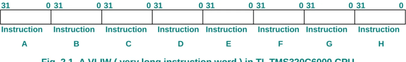
(12) Chapter 2. Fundamental Background and Related Work In this chapter, we will introduce the fundamental background of the problem and some basic definitions. Then the power cost function will be presented. Third, we will introduce some related work, including MSAS (Minimizing Switching Activities Scheduling), Horizontal and Vertical Scheduling, PRRS (Power Reduction Rotation Scheduling), and SAMLS (Switching-Activity Minimization Loop Scheduling). Finally, we will give a briefing of our motivation.. 2.1 Fundamental Background[8-10]. A long instruction is a very-long instruction word executed by a VLIW CPU during each clock cycle. Sub-instructions are several parallel instructions composing long instruction. Fig. 2.1 shows that what is a long instruction and what is a sub-instruction. In a TI TMS320C6000 CPU, it can execute up to eight 32-bit instructions per cycle since the C6000 core CPU consists of eight functional units[8]. In Fig. 2.1, from instruction A to instruction H, each one is a 32-bit instruction that can be executed simultaneously. Hence, there are eight sub-instructions in Fig. 2.1, and eight sub-instructions compose one long instruction.. 31. 0 31. Instruction A. 0 31. 0 31. Instruction. Instruction. B. C. 0 31. 0 31. Instruction Instruction D. E. 0 31. 0 31. Instruction Instruction F. G. Fig. 2.1 A VLIW ( very long instruction word ) in TI TMS320C6000 CPU. 3. 0. Instruction H.

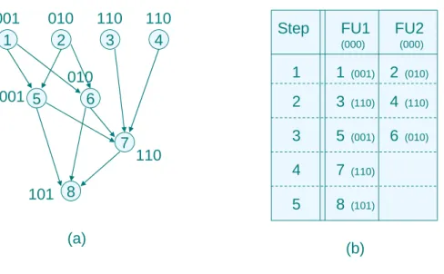
(13) 001 1. 010 2. 001 5. 110 3. 110 4. Step. 010 6 7. FU1. FU2. (000). (000). 1. 1. (001). 2. (010). 2. 3. (110). 4. (110). 3. 5. (001). 6. (010). 4. 7. (110). 5. 8. (101). 110. 101 8 (a). (b). Fig 2.2(a) A given DAG ; (b) A schedule of left DAG. After knowing what a sub-instruction is, we will use it in the following definition, which is an important input of our algorithm.. Definition 2.1. A Directed Acyclic Graph (DAG) G=(V, E, Bit_String(u) ) is a node-weighted graph, where V is the set of nodes and each node represents a sub-instruction, and E is the edge set and an edge between two nodes denotes a dependency relation, and Bit_String(u) is a function to represents the machine code for each node u ∈ V. A DAG is an input of our algorithm. Fig 2.2(a) is an example of DAG. From node 1 to node 8, each node is a sub-instruction and belongs to V. Each edge between two nodes denotes the dependency relation. For example, node 6 could not be executed before node 1 and node 2 are executed. The binary strings beside the nodes are their machine code. Hence, Bit_String(node 5) is 001 and Bit_String(node 7) is 110.. Definition 2.2. The location of a node in a schedule of a DAG is a two dimensions array. Each element of this array is a sub-instruction. Fig 2.2(b) is a schedule of Fig 2.2(a). We use (i, j) to denote the location of a sub-instruction in a schedule, where i is the row and j is the column. The row number 4.

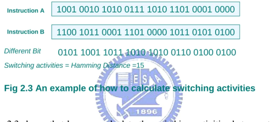
(14) represents the clock cycle in which the sub-instruction is executed. The column number represents the functional unit on which the sub-instruction is executed. For example the location of node 6 is (3, 2). On the other hand, we can use (3, 2) to represents node 6.. Next, we will introduce what is switching activities. Basically, it is one of the most important factors of calculating the consumption of power[10]. Switching activities is the Hamming Distance of two consecutive instructions. Hamming Distance is the number of bit differences between two binary strings.. Instruction A. 1001 0010 1010 0111 1010 1101 0001 0000. Instruction B. 1100 1011 0001 1101 0000 1011 0101 0100. Different Bit. 0101 1001 1011 1010 1010 0110 0100 0100. Switching activities = Hamming Distance =15. Fig 2.3 An example of how to calculate switching activities. Fig 2.3 shows that how we calculate the switching activities between two instructions. We suppose that instruction A and instruction B are two contiguous sub-instructions on the same functional unit and the binary strings are their machine code. We can observe that the number of different bit of two binary strings is 15, so the switching activities of two instructions is 15.. 2.2 Power Cost Function. In this section, we will introduce the energy consumption equation based on the energy model proposed by [10]. We will use this energy model to evaluate our method. As we mention before, a VLIW processor executes a long instruction during each clock cycle. A long instruction is composed of several parallel sub-instructions. The power. 5.

(15) onsumption to execute a long instruction during a clock cycle, Pcycle, can be computed by :. Pcycle = Pbase + ∑ { PInsti + SP (i, j)}. (1). Insti. where Pbase is the base power needed to support a long instruction execution even when a long instruction contains only NOPs. Pinsti is the power to execute a sub-instruction Ii on a functional unit, and SP(i, j) is the switching power caused by switching activities between Insti (current sub-instruction) and Instj(last sub-instruction) executed on the same functional unit. The switching power is proportional to the number of transitions. So. SP (i, j) = α . WHD( Bit_String(Inst_i), Bit_String(Inst_j) ). (2). where α is a power coefficient representing the consumed power per transition, and WHD (Weighted Hamming Distance) is a function used to compute the number of transitions between Insti and Instj. Let X = Bit_String(Insti) and Y = Bit_String(Instj), and WHD(X, Y) is : K. WHD( X, Y ) = ∑ wi . (X [i] ⊕ Y [j] ) (3) i=1. Where wi is the weight of a transition. wi is used to denote the weight for power consumption caused by one transition on different units. The energy consumption of a program is the summation of all its power consumption during each clock cycle. Let S be a schedule for an application and L the schedule length of S. Then the energy consumption of schedule S, Es, can be computed by. L. L. L. (K). Es = ∑ Pcycle = L* Pbase + ∑ ∑ PInsti + ∑ ∑ SP (i, j)} (K). K=1. K=1. Insti. (K). K=1 Insti. (4). (K). ∑∑P is the summation of basic power consumptions for all sub-instructions of an application that does change with different schedules. Pbase is a constant and Pbase * L varies with schedule length for specific VLIW processor. ∑∑SP(i,j) is the switching power and changes with 6.

(16) different schedules. Therefore, schedule length and switching activities need to be considered together in instruction-level scheduling techniques in order to minimize energy consumption of a program.. 2.3 Related Work[11-13][19]. In this section, we’ll show how Minimizing Switching Activities Scheduling (MSAS) works, and then Horizontal and Vertical Scheduling will also be introduced. Finally, we will introduce. Power. Reduction. Rotation. Minimization Loop Scheduling (SAMLS). Scheduling. (PRRS). and. Switching-Activity. .. 2.3.1 Minimizing Switching Activities Scheduling[12]. The algorithm, Minimizing Switching Activities Scheduling (MSAS), was designed to solve a special case of instruction-level energy-minimization scheduling, i.e., the case when switching activities play the most important role in energy consumption. When Pbase is very small compare with α ( in equation 2 in section 2.2 ), the energy of a schedule depends mainly on switching activities. For example, when Pbase equals 0.1 and α equals 1, then we need to reduce 10 control steps in schedule length to count one bit switch. Thus, the MSAS algorithm was designed to minimize switching activities as much as possible. On the other side, considering the performance, the algorithm also wants to minimize schedule length. Hence, MSAS algorithm minimizes switching activities in first priority and still considers schedule length. Since most previous work focus on one functional unit, the algorithm takes advantage of multiple functional units under VLIW architectures. In this algorithm, the input is the DAG we have defined it in previous section and the 7.

(17) output is a schedule with switching activities minimization. Due to the existence of the dependency in DAG, we can only schedule a node after all its parent nodes have been scheduled. The scheduling problem with switching activities minimization is how to find a matching between functional units and ready nodes in such a way that it can minimize the total switching activities in every scheduling step. This is equivalent to the min-cost weighted bipartite matching problem. Thus, in the first scheduling step of MSAS algorithm, it creates a weighted bipartite graph GBM, where the vertices of one side are the set of the functional units and the vertices of the other side are the nodes in ready list and the weight of the edge between the node and the functional unit is the switching activities when the node is assigned to the functional unit. Then it assigns nodes based the min-cost maximum bipartite matching. After assigning the nodes, it updates the nodes in the ready list according to the DAG and the machine codes of the functional units. Then it repeatedly creates the weighted bipartite graph and assigns the nodes until all the nodes are scheduled. The schedule created by MSAS can reduce total switching activities since it considers the min-cost maximum bipartite matching in each step. It is know that finding a min-cost maximum bipartite matching take O(n3) by the Hungarian Method[20]. Let N be the number of functional unit. In every scheduling step, it needs at most O((N+|V|)3) to find minimum weight maximum bipartite matching using Hungarian Method and the scheduling step is at most |V|. Thus, the complexity of MSAS is O(|V|*(N+|V|)3). It takes too much time to find minimum weight maximum bipartite matching and it may not find the minimal switching activities in some cases. We will show you in our motivation.. 2.3.2 Horizontal Scheduling and Vertical Scheduling[13]. Both high performance and low power are two important objectives of complier optimization. Thus, in [13], the authors propose a two-phase instruction scheduling approach. 8.

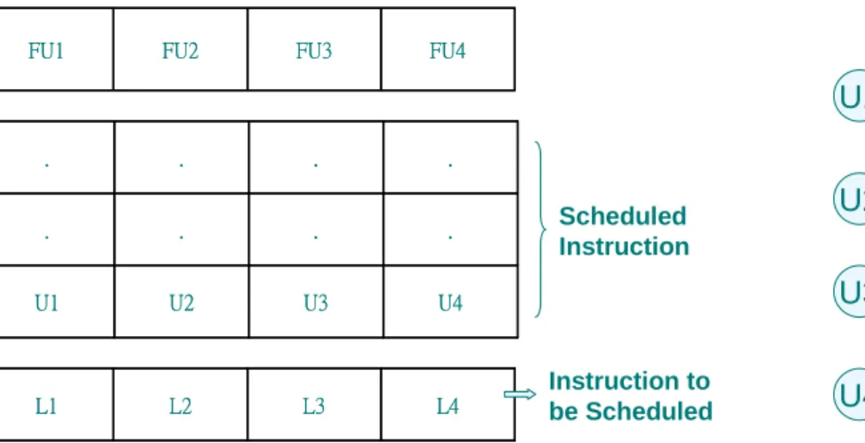
(18) In the first, instructions are scheduled by list schedule for performance. Then, in the second phase, horizontal and vertical scheduling methods are employed to re-arrange the codes reducing the power without incurring performance penalty. We first introduce the horizontal scheduling algorithm which re-schedules the instruction components of a long instruction to minimize switching activities of instruction bus. Suppose we have n VLIW instructions which have been scheduled by list schedule, then the horizontal scheduling won’t change the control step of each long instruction and the component of each long instruction, but it will try to re-arrange the position of each sub-instruction of a long instruction to reduce the switching activities. The way of re-schedule the position of sub-instructions of a long instruction is to create the weighted bipartite graph GBM between the long instruction which is re-scheduled and the long-instruction is considered to re-schedule right now. In GBM, the vertices of two sides are the sub-instructions of two long instructions and the weight of the edge is the switching activities between two sub-instructions. Like as MSAS, the horizontal scheduling finds the min-cost maximum bipartite matching and re-arranges the position of each sub-instruction according to the min-cost maximum bipartite matching. For example, in figure 2.4, U1 to U4 are the sub-instructions in the last long instruction already scheduled and L1 to L4 are the sub-instructions of a long instruction to be re-scheduled. Thus, it creates bipartite matching between them and finds the min-cost maximal matching. Then it re-schedules the positions of L1 to L4 according to the matching. This algorithm repeatedly creates weighted bipartite graph and re-arranges the positions of the sub-instructions of each long instruction from the first long instruction to the last long instruction in the schedule created by list schedule. After re-scheduling all the long instructions, we can get a schedule which has less total switching activities. Next, we will introduce the vertical scheduling. The vertical scheduling is similar with horizontal scheduling, but it allows sub-instructions to move across long instructions. 9.

(19) FU1. FU2. FU3. FU4. .. .. .. .. .. .. .. .. U1. U2. U3. U4. L1. L2. L3. L4. Scheduled Instruction. Instruction to be Scheduled. U1. L1. U2. L2. U3. L3. U4. L4. Fig. 2.4 An example of bipartite matching for horizontal scheduling. That is, the horizontal scheduling won’t change each sub-instruction’s control step but the vertical scheduling. How can vertical scheduling do this? Because it uses a window size w to decide the weighted bipartite graph between the sub-instructions in the last long instruction already scheduled and the sub-instructions in the next w long instructions that satisfy data dependence constraint. We can say that horizontal scheduling is a special case of vertical scheduling when the window size w = 1. Like as the horizontal scheduling, the vertical scheduling finds the min-cost maximum bipartite matching and re-arranges the position of each sub-instruction according to the min-cost maximum bipartite matching repeatedly until all sub-instructions are scheduled. The two algorithms present the essential idea of their low power optimization. It requires the functional units of target VLIW architectures to be identical. Thus, they can only perform sub-instructions swapping with identical functional units on target host without performance penalty. However, the functional units are normally classified into several classes in most of VLIW architecture designs. The swapping can only be done with functional units of the same class. This is the main constraint of their method.. 10.

(20) 2.3.3 Power Reduction Rotation Scheduling[11]. The algorithm, Power Reduction Rotation Scheduling, was designed to minimize both switching activities and scheduling length for loop applications and is based on rotation scheduling[3]. Rotation Scheduling presented in[3] is a scheduling technique used to optimize a loop schedule with resource constraints. The main goal of rotation scheduling is to reduce the schedule length of a loop application. It transforms a schedule to more compact one iteratively. Retiming[21] can be used to break the intra-dependence between instructions in a loop application, so that the rotation can be done to reduce the schedule length of a loop application. In each step of rotation, nodes in the first row of the schedule are rotation down. By doing so, the nodes in the first row are re-scheduled to the earliest possible available locations. From retiming point of view, each node gets retimed once by drawing one delay from each of incoming edges of the node and adding one delay to each of its outgoing edges in the DFG. The new location of the node in the schedule must also obey the precedence relation in the new retimed graph. The Power Reduction Rotation Scheduling is totally based on rotation scheduling. In addition, each node needed to be rotated must to be scheduled on the location with minimum switching activities. So it can achieve the goal to reduce power consumption. The disadvantage of PRRS is that it was designed for the loop application and it can not be use in none loop application. It needs an initial schedule to be its input and it takes extra time to create the initial schedule.. 2.3.4 Switching-Activity Minimization Loop Scheduling[19]. Switching-Activities Minimization Loop Scheduling is an improving algorithm of PRRS 11.

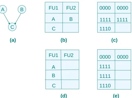
(21) which was developed to reduce both schedule length and switching activities of a loop application. Switching-Activity Minimization Loop Scheduling (SAMLS) was based on rotation scheduling and bipartite matching. In the first phase of SAMLS, it performed the same thing as PRRS did. Then the schedule created by phase one will be the input of the phase two of SAMLS. In the phase two of SAMLS, it performed the same thing as horizontal scheduling did. As the results of experiments, SAMLS has a little better performance than that of PRRS in reducing switching activities, but SAMLS takes much more time than that of PRRS.. 2.4 Motivation. From the relative work, we can observe that reducing the switching activities is an important factor of reducing total power consumption, especially when switching activities play the most important role in energy consumption. Hence, we focus our working on reducing switching activities as much as possible, despite it may take more control steps to complete the application. In section 2.3.1 and section 2.3.2, we can see that both algorithms create weighted bipartite graph. Then MSAS finds the min-cost maximum bipartite matching and horizontal scheduling finds the maximum bipartite weighted matching.. Both of them try to find the. minimal switching activities in each allocation. We can observe that it may not find the minimal switching activities. For example, figure 2.5(a) is a simple example of DAG., and figure 2.5(b) is the schedule of figure 2.5(a) by using MSAS. Assuming the binary strings in Figure 2.5(c) are the machine codes of these instructions. Then the switching activities is 9. But in figure 2.5(d) and figure 2.5(e), we can find that another schedule will cost less switching activities. We can observe that instruction A and instruction B have the same. 12.

(22) A. B. C. FU1. FU2. 0000. 0000. A. B. 1111. 1111. C. (a). 1110 (b). FU1. (c). FU2. 0000. A. 1111. B. 1111. C. 1110 (d). 0000. (e). Fig 2.5 (a) A DAG ; (b) the schedule of (a) with MSAS ; (c) switching activities = 9 (d) other schedule of (a) ; (e) switching activities = 5. machine code in this case. If we use MSAS to schedule it, we lost the benefit of scheduling B instruction after A instruction. In addition, in actual VLIW architectures, different functional units perform different functions. For example, a load instruction can be executed in specific unit and so is a multiply instruction. Hence, it is not a good way to find min-cost maximum bipartite matching in an architecture while the functional units are not identical. Therefore we try to find a better way to schedule the applications to reduce power consumption in real VLIW architectures. Another important motivation is that how to assign registers to reduce switching activities in MSAS or other algorithm is not considered. We will also try to find a better way to assign registers to achieve further reducing the switching activities. Moreover, finding a min-cost maximum bipartite matching takes too much time. The complexity of MSAS is O(|V|*(N+|V|)3), where N is the number of functional units and V is the number of nodes. Thus, we will also consider of reducing the complexity of our scheduling algorithm. In the next chapter, we will describe the basic concepts and principles of our method in some detailed.. 13.

(23) Chapter 3. Greedy Switching Activities Scheduling In this chapter, we will first introduce our experimental machine architecture. Then our proposed method, GSAS (Greedy Switching Activities Scheduling), will be presented. We will use an example to explain our GSAS in some detail. We will also analyze our algorithm compared with MSAS[12].. 3.1 Machine Architecture. The architecture of our experimental VLIW processor is based on TI TMS320C6K processor, since it is commonly used in image processing, multimedia, wireless security, etc[8-9]. There are multiple functional units executed simultaneously in these architectures, power consumption becomes one of the most important issues to be considered with the concern of performance. Thus, we choose TI TMS320C6K processor to be the base of our experimental model. We will first introduce the architecture of TI TMS320C6K processor. Then we will introduce our proposed machine for our experiments.. 3.1.1 Architecture of TM320C6K[8-9]. The architecture of TMS320C62X/C64X/C67X processor is shown in Figure 3.1. The CPU contains program fetch unit, instruction dispatch unit, advanced instruction packing(C64 only), instruction decode unit, two data paths and each with four functional units, 32 32-bit registers or 64 32-bit registers (C64 only), control registers, ontrol logic, test, emulation and interrupt logic. The program fetch, instruction dispatch, and instruction decode units deliver up to eight 32-bit instructions to the functional units every CPU clock. The processing of instructions 14.

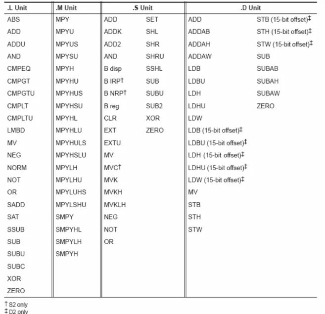
(24) Fig 3.1 TMS320C62X/C64X/C67X Block Diagram. occurs in each of the two data paths (A and B), each of which contains four functional units and 16 32-bit general-purpose registers for the C62X/C67X and 32 32-bit general-purpose registers for C64X. As for functional units, there are eight functional units in the architecture. The eight functional units in the C6000 data paths can be divided into two groups of four; each functional unit in one data path is almost identical to the corresponding unit in the other data path. The functional units are named .L, .M, .S, and .D. Figure 3.2 shows the mapping between instructions and functional units.. 15.

(25) Fig 3.2 Instruction to functional unit mapping. In figure 3.1, we can see that there are two general-purpose register files (A and B) in the C6000TM date paths. For the C62X/C67X DSPs, each of these files contains 16 32-bit registers (A0-A15 for file A and B0-B15 for the file B). The general-purpose registers can be used for data, data address pointers, or condition registers. The C64X DSP register file doubles the number of general-purpose registers that are in the C62X/C67X cores, with 32 32-bit registers (A0-A31 for file and B0-B31 for file B). Each functional unit read directly from and writes directly to the register file within its. 16.

(26) Fig. 3.3 TMS320C62X/C64X/C67X Opcode Map. own data path. That is, the .L1, .S1, .D1, and .M1 units write to register file A and the .L2, .S2, .D2, and .M2 units write to register file B.. 3.1.2 Proposed Machine Architecture. In our experimental machine architecture, we use a simplified model based TMS320C6000 described in previous section. We used the same functional units and data 17.

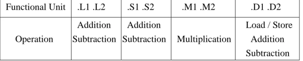
(27) Functional Unit. Operation. .L1 .L2. .S1 .S2. .M1 .M2. Addition Addition Subtraction Subtraction. Multiplication. .D1 .D2 Load / Store Addition Subtraction. Table 3.1 Functional units of proposed machine architecture. Machine Code Field Load. op(10000). memory address (10bit). dst (5 bit). Store. op(10100). memory address (10bit). src (5 bit). Addition. op(01000). src1 (5 bit). src2 (5 bit). dst (5 bit). Subtraction. op(01100). src1 (5 bit). src2 (5 bit). dst (5 bit). multiplication op(00000). src1 (5 bit). src2 (5 bit). dst (5 bit). Table 3.2 Machine code of each instruction. paths, but with the simplified instructions. Based on the opcode of the instruction set[8] in the Fig 3.3, we can find that the most important factors affecting the machine code are the destination, source1, source2, and operate fields. The symbol creg and z represent the conditional registers. In most case, the conditional registers are not used. The symbol s means select side A or B for destination. In the counting of switching activities, it won’t cause switching on the same side. The symbol p represents the parallel execution. We can’t decide its’ value until the schedule have been done. Hence, we delete those fields and preserve the fields of destination, source1, source2, and operate. In most DPS benchmarks, the additions and multiplications are executed frequently. Hence, we preserve the instructions of addition, multiplication, subtraction, load, and store in our experiments. Table 3.1 shows the mapping between instructions and functional units. Table 3.2 shows the machine codes of each instruction. The machine codes of all instructions. 18.

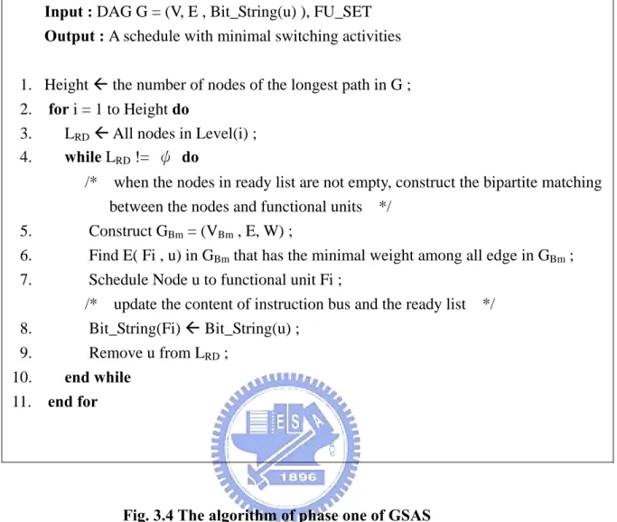
(28) in our proposed architecture are 20 bits binary strings. The symbol src represents the source and dst represents the destination and they are 5 bits binary strings. The registers can be used in the fields of src or dst. In our proposed architecture, 32 registers (A0-A15 for file A and B0-B15 for the file B) can be used. It is the same as C62X/C67X processors. The machine codes of register file A are from 00000 to 01111, and the machine codes of register file B are from 10000 to 111111. The machine codes of memory address are from 0000000000 to 1111111111.. 3.2 Greedy Switching Activities Scheduling. In this section, we will introduce our algorithm, GSAS (Greedy Switching Activities Scheduling), which is an effective method to reduce the switching activities in scheduling applications. GSAS consists of two phases. The first phase is to arrange the schedule. In other word, the first phase will decide what location and cycle the sub-instructions should be placed. After deciding the schedule, the second phase can be executed. The goal of second phase is to re-assign the registers to reduce the switching activities.. 3.2.1 Phase One of GSAS. In this section, we will introduce phase one of our algorithm, GSAS (Greedy Switching Activities Scheduling). The word “greedy“ is the main principle of our method. As we mention in the section 2.4, the drawback of MSAS is that it may neglect some situation which will cause less switching activities. Moreover, it takes much time to find a min-cost maximum weight bipartite matching. Hence, we use a greedy method to choose the sub-instruction which will cause the minimal switching activities. The figure 3.4 shows the phase one of GSAS. The input of the algorithm is a DAG and the functional unit set. The output of the algorithm is a schedule with minimal switching 19.

(29) Input : DAG G = (V, E , Bit_String(u) ), FU_SET Output : A schedule with minimal switching activities 1. Height Å the number of nodes of the longest path in G ; 2. for i = 1 to Height do 3. LRD Å All nodes in Level(i) ; 4. while LRD != ψ do /* 5. 6. 7. 8. 9.. when the nodes in ready list are not empty, construct the bipartite matching between the nodes and functional units */ Construct GBm = (VBm , E, W) ;. Find E( Fi , u) in GBm that has the minimal weight among all edge in GBm ; Schedule Node u to functional unit Fi ; /* update the content of instruction bus and the ready list */ Bit_String(Fi) Å Bit_String(u) ; Remove u from LRD ;. 10. end while 11. end for. Fig. 3.4 The algorithm of phase one of GSAS. activities. We will introduce it in the following. We first define some symbols in our algorithm. We use Level(i) to represent the. set of. nodes, where i represents the critical path of the nodes according to data dependency. For example, in Figure 3.5 (a), node 1 to 2 belong to Level(1) since these nodes have no parent. Node 3, Node 4, and Node 5 belong to Level(2) since these nodes couldn’t be executed until some nodes in Level(1)have been executed. Hence, node 6 and node 7 are in Level(3) and so on. Height represents the number of the nodes of the critical path of the DAG. For example, in Figure 3.5 (a), the Height is 4. LRD represents the nodes ready to be scheduled. As we mention in our motivation, we focus our working on reducing switching activities as much as possible, and it may take more control steps to complete the application. We 20.

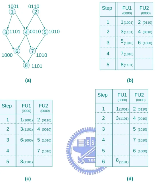
(30) schedule the DAG level by level. It can assure that the nodes in high level will be scheduled first and avoid creating schedule with too long length. In this algorithm, we schedule the nodes level by level. In line 3, we first assign the nodes in Level(1) to the ready list. When the ready list is not empty, we construct the weighted bipartite matching GBm = ( VBM, E, W ), where VBM = FU_SET ∪ LRD where FU_SET = < F1, F2,…,FN> is the set of all functional units and LRD is the set of all nodes in ready list . For each functional unit Fi ∈ FU_SET and each node u ∈ LRD, an edge e(Fi, u) is added into E and the weight of e(Fi, u), W(Fi, u) = WHD(β, Bit_String(u), Bit_String(Fi)) and Bit_String(Fi) = Bit_String(v) where v is the last node executed on Fi. WHD(β, X, Y) is the weighted hamming distance function and is the same as WHD( X, Y) in equation 3 besides a new parameter β. We use the parameter β represents the first β bits in the binary string. In the WHD(β, X, Y), we only calculate the hamming distance of the first β bits between two binary strings. We do this because we will re-assign the register used by the destination of the sub-instructions in phase two. Therefore, we only consider the fields of op, src1, src2, and memory address of the machine codes of the sub-instructions in Table 3.2 and the value of β will be 15. It will increase the probability of operand sharing. The value of β will be 20 if we only use phase one and do not re-assign the registers. We will use an example to demonstrate our method and show the benefit of our algorithm. After constructing the GBM, we use a greedy method to choose the minimal weight edge and schedule the node. After scheduling the node, then we update the nodes in the ready list and the content of the instruction bus. We repeatedly choose the node from the ready list until all the nodes in the ready list are scheduled. When the ready list is empty, we assign the nodes in the next level to the ready list and repeat the step we did it before until all nodes in the DAG are scheduled. Let’s use a simple example to demonstrate our method. Since the machine codes of the sub-instructions are 4 bits, we calculate all the bits in hamming distance and β is 4 in 21.

(31) 1001 1. 0110 2. Step. 3 1101 4 0010 5 1010. 1000. 7. 6. FU1. FU2. (0000). 1010. 8 1101. (0000). 1. 1 (1001) 2. (0110). 2. 3 (1101) 4. (0010). 3. 5 (1010) 6. (1000). 4. 7 (1010). 5. 8 (1101) (b). (a) Step. FU1. FU2. (0000). Step. FU1. FU2. (0000). (0000). (0000). 1. 1 (1001) 2. (0110). 1. 1 (1001) 2. (0110). 2. 3 (1101) 4. (0010). 2. 3 (1101) 4. (0010). 3. 5. (1010). 3. 6 (1000) 5. (1010). 4. 7. (1010). 4. 7. (1010). 5. 6. (1000). 5. 8 (1101). 6. 8 (1101). (d). (c). Fig. 3.5 (a) A DAG ; (b) list schedule with total SA = 14 , SL = 5 ; (c) MSAS with total SA = 11 , SL = 5 ; (d) GSAS with total SA = 8 , SL = 6. WHD(β, X, Y). Figure 3.5(a) is a DAG. According to the algorithm of the phase one of GSAS, node 1 and node 2 will be in the LRD first since they are in Level(1). Then we construct the edges between the ready nodes and the functional units and weight of the edges are both 2. We schedule node 1 on FU1 first and there is only node 2 in LRD. Hence, we construct the edges between node 2 and functional units. The weight of the edge connected to FU1 is 4 and the weight of the edge connected to FU2 is 2. Thus, we schedule node 2 on FU2. By the same way, we can schedule the nodes in Level(2) and so on until all the nodes are scheduled. Figure 22.

(32) 3.5(b)~(d) are the schedules of different algorithms. In those figures SA stands for switching activities and SL stands for schedule length. From the result, we can see that phase one of GSAS has the better performance in reducing switching activities. Let’s compare the schedule of MSAS with the schedule of phase one of GSAS. We can see that both algorithms have the same schedule in the first two control steps. In the control step 3, MSAS has to find the min-cost maximal weight bipartite matching, so it has to schedule the node 6 at (3, 1) and schedule the node 5 at (3, 2). Hence, in the control 4, MSAS only can schedule the node 7. But when we use GSAS to schedule the nodes, we can only schedule node 5 at (3, 2) in the control step 3 since it causes the minimal switching activities. Hence, in the control step 4, GSAS can choose the best option from node 6 and node 7 which can be scheduled after node 3 or node 5. Obviously, scheduling node 7 at (4, 2) causes the least switching activities. Then, in the control step 5, scheduling node 6 at (5, 2) causes the least switching activities and is better than that of scheduling it at (3, 1). Therefore, GSAS can avoid the disadvantageous arrangement caused by schedule more than one node in one iteration. Moreover, the complexity of MSAS is O(|V|*(N+|V|)3), where |V| is the number of the sub-instructions and N is the number of functional units. But the complexity of phase one of GSAS is (|V|*(|V|*N)), since instead of finding the min-cost maximal weight bipartite matching, we just finds the only one node in one iteration which needs at most O(|V|*N) to be completed. Hence, the phase one of GSAS saves more time in comparing with MSAS.. 23.

(33) Input : DAG G = (V, E , Bit_String(u)), schedule S Output : A new DAG G’ =(V, E, Bit_String’(u)) 1. all src and dst in V Å NULL; 2. Height Å the number of nodes of the longest path in G ; 3. for i = 1 to Height do 4. LRA Å all the nodes in Level(i) ; 5. while LRA != ψ do 6. 7.. u Å the node has minimal time(v) for each v∈ LRA; unlock(all registers); /*. 8. 9. 10. 11. 12. 13. 14.. lock all register if assigning it to the u.src will cause data hazard */. lock(v.src) for each v∈ V and time(v) > time (u) ; find the register Ai will cause the minimal switching activities when assigning it at dst of u /* from all the registers which are not locked */ u.dst Å Ai ; re-assign src of all children of u ; end while end for. Fig. 3.6 The algorithm of phase two of GSAS. 3.2.2 Re-assign the Registers by the Phase Two of GSAS. In this section, we will introduce the phase two of GSAS. The main goal of phase two is to re-assign the registers used by the src and dst in each sub-instruction to reduce the switching activities of the schedule created by phase one of GSAS. The. meaning of. symbol src and dst have been introduced in section 3.1.2. In previous work of[11-13], they didn’t consider about how to assign the registers to reduce the switching activities. Actually, the register assignment is an important factor affecting the component of the machine codes of sub-instructions. Thus, we use the phase two 24.

(34) of GSAS to re-assign the registers to reduce the switching activities. Figure 3.6 shows the phase two of GSAS. The input of the algorithm is the DAG and the schedule produced by the phase one of GSAS and the output of the algorithm is the DAG with different registers used by each sub-instruction. The DAG with new machine codes reduces the switching activities of the schedule produced by the phase one of GSAS. We first define some symbols in our algorithm. In the algorithm, the meanings of Level(i) and Height are the same as that of the phase one. LRA represents the list of nodes to which the registers are re-assigned. u.dst represents the register of destination of u and u.src represents the register of source of u. We use two functions lock() and unlock() to decide the state of the registers. If the state of the register is locked, then it couldn’t be used; otherwise it can be re-assigned. With the lock() and unlock(), data hazard can be avoided. The function time() returns the control step of the node in schedule S. In the algorithm, Line 1 sets the registers in all sub-instructions to be null in the first. Line 3 re-assigns the registers of the nodes level by level. In this sequence, data dependence won’t be violated. In the first, the nodes in Level(1) will be assigned to LRA. Then we choose the first node to re-assign register to it in line 6 and u represents the node. We will assign the register which will cause minimal switching activities to dst of u. Before we choose the register, we should unlock all registers and then we lock all the registers which may cause data hazard in line 7 and line 8. From line 9 to line 11, we scan the register file and find the register to cause the minimal switching activities when assigning it at dst of u. That is, assigning it to dst of u will make the switching activities between the field of destination of u and the previous sub-instruction on the same functional unit minimal. Figure 3.7 show the detail of how to assign the register. Line 12 updates the src of the children of u. according to the DAG. Then, the first iteration of the algorithm is done. According to input of the schedule, we can find the next node. After we have re-assigned registers to all the nodes in Level(1), we can consider the 25.

(35) Input : current sub-instruction u and last sub-instruction v on the same functional unit Output : register Ai 1.. RÅ number of registers , Min Å ∞ ;. 2. 3 4. 5. 6. 7. 8. 9.. for i = 0 to R-1 do if Ai is not locked then if WHD(Bit_String(u.Ai), Bit_String(v.dst)) < Min ; then RegÅ Ai ; end if end if end for return Reg ;. Fig. 3.7 The algorithm of register assignment. 1 ld (Ar) A0 2 ld (Ai) A1 3 ld (Br) A2 4 ld (Bi) A3 5 ld (Cr) A4 6 ld (Ci) A5 7 mul A0 A2 8 mul A1 A3 9 mul A0 A3 10mul A1 A2 11add A6 A4 12add A8 A5 13sub A10 A7 14add A11 A9 15 st (Dr) A12 16 st (Di) A13. 1. Level(1). A6 A7 A8 A9 A10 A11 A12 A13. Level(2). 2. 7. Level(3). 8. 4. 9. 11. Level(4) Level(5). (a). 3. 5. 6. 10. 12 13. 14. 15. 16 (b). Fig 3.8 (a) Assembly code of complex_update ; (b) DAG of complex_update. 26.

(36) .S1. .L1. .M1. 1 ld (Ar) A3 2 ld (Ai) A2 3 ld (Br) A0 4 ld (Bi) A1 5 ld (Cr) A3 6 ld (Ci) A1 7 mul A3 A0 8 mul A2 A1 9 mul A3 A1 10mul A2 A0 11add A4 A3 12add A5 A1 13sub A8 A4 14add A9 A0 15 st (Dr) A1 16 st (Di) A1. .D1 3 4 1. 7. 2. 9. 5. 11. 8. 6. 12. 10. 13 14. 15 16. A4 A4 A5 A0 A8 A9 A1 A1. (d). (c). Fig 3.8 (c) schedule of the phase one of GSAS ; (d) Assembly code of complex_update after phase two. nodes in Level(2) and so on. Let’s use an example to demonstrate our algorithm of phase two. This example performs a complex update of the form D = C + A*B where A, B, C and D are complex numbers. We first assign the dst of the nodes in a common way: from A0 to A15. Figure 3.8 (a) shows the initial assembly code of complex update. Figure 3.8 (b) is the DAG of complex update. Figure 3.8 (c) is the schedule created by the phase one of the GSAS. In the phase one, the value of β in WHD (β, X, Y) is 15 since we will re-assign the register of the destination of a node. We only consider about the first 15 bits of the binary string. In figure 3.8 (c) we can find the benefits of using the phase one of GSAS. Node 7, 8, 9, 10 are scheduled in this sequence “7, 9, 8, 10”. They are scheduled in the sequence since we choose the node which will cause minimal switching activities to schedule. That will increase the probability of operand sharing. After the phase one of GSAS, we can re-assign the registers. According to the DAG, 27.

(37) node 1 to 6 will be considered first. Node 3 will be re-assigned first since its control step is 1 and we assign A0 to the dst of node 3 since A0 cause the minimal switching activities. Then we will re-assign register to dst of node 4. Before we re-assign the register we should lock some register. According to the DAG and the schedule, the src of node 7 and node 10 will use the register A0 and the numbers of control steps of them are more than that of node 4, therefore we lock A0 and A0 can not be assigned to dst of node 4. A1 will be assigned to the dst of node 4. By the same way, we can re-assign all the nodes and the new registers will reduce the total switching activities. Figure 3.8(d) shows the assembly code of complex update after we re-assign the registers. The complexity of the phase two of GSAS is O(|V||*(|V|+R), where |V| is the number of nodes and R is the number of the registers. It needs O(|V|) to lock registers in line 8 and O(R) to find the register in one iteration. It needs |V| iteration to re-assign all nodes. Hence, the complexity is O(|V||*(|V|+R). In this chapter, we have demonstrated our method in some detail. In the next chapter, we will see the experimental results and some analyses about our experiments.. 28.

(38) Chapter 4. Preliminary Performance Evaluations In this chapter, we will demonstrate our experimental results. The machine architecture of our experiments has been introduced in chapter 3. The benchmarks of our experiments are from DSPstone[23]. We will first compare the results of phase one of GASA with the results of other methods. Then we will evaluate the results of phase one of GSAS with the results of phase one and two of GSAS.. 4.1 The Experimental results for phase one of GSAS In this section, we will illustrate our experimental results of phase one of GSAS. In Table 4.1, it shows the schedule length and switching activities of each benchmark for each method. We can find that list schedule has the shortest schedule length in comparing with other methods. Our method, the phase one of GSAS, has the least switching activities in each benchmark although it may have the longer schedule length. From the section 2.2, we found that schedule length and switching activities are two important factors affecting the power consumption. Two constant Pbase and α play important role in calculating the total energy consumption in equation (4). Therefore, we change the value of Pbase and α to consider different situations. When Pbase is bigger than α, it means that schedule length plays the most important role in energy consumption. Conversely, when α is bigger than Pbase, it means that switching activities play the most important role in energy consumption Table 4.2 to 4.6 show the total energy and reduction compared with list schedule. We use different value of Pbase and α to calculate the total energy. We can find that the more Pbase is bigger than α, the less reduction in our method. But when α is bigger than Pbase, we have a better performance in reducing total energy consumption since switching activities play an 29.

(39) List Schedule complex_multiply dot_product real_update complex_update biquad_one_section fir mat1X3 convolution. SL. SA. SL. SA. SL. SA. SL. SA. SL. SA. SL. SA. SL. SA SL. SA.. 9 50 7 41 5 33 9 80 13 111 12 59 21 137 8 66. MSAS 9 44 7 32 5 27 10 69 15 97 12 51 21 113 8 58. Phase I 11 40 8 28 5 27 12 65 14 84 13 48 23 102 8 58. Table 4.1 The comparison on the schedule length and the switching activities important factor in affecting power consumption. In Figure 4.1, the row is (Pbase, α) and the column is the percentage of total energy based on list schedule. From figure 4.1 (a) to (h), we can see the reduction in total energy for each method clearly. In all figures, GASA have more reduction in total energy than that of MSAS when α is bigger than Pbase. But in figure 4.1 (a), (b), (d), (f), we can find that phase one of GASA is worse than MSAS when (Pbase, α) = (5, 1). For the phase one of GSAS, it has the longer schedule length than that of MSAS while Pbase is much bigger than α. Hence, GSAS is not as good as MSAS. In figure 4.1 (c), (h), MSAS and the phase one of GSAS have the same results since they have the same schedule. Thus, we can find that our method has the better benefit of reducing switching activities and reduced more power while α is bigger.. 30.

(40) complex_multiply dot_product real_update complex_update biquad_one_section fir mat1X3 convolution. List Schedule. MSAS. 59 -48 -38 -89 -124 -71 -158 -74 --. 53 10.2 39 18.8 32 15.8 79 11.2 112 9.7 63 11.3 134 15.2 66 10.8. E. Reduction E. Reduction E. Reduction E. Reduction E. Reduction E. Reduction E. Reduction E. Reduction. Phase I 51 13.6 36 25 32 15.8 77 13.5 98 21.0 61 14.1 125 20.9 66 10.8. Table 4.2 The comparison on energy when Pbase = 1 and α = 1. complex_multiply dot_product real_update complex_update biquad_one_section fir mat1X3 convolution. List Schedule. MSAS. 68 -55 -43 -98 -137 -83 -179 -82 --. 62 8.8 46 16.4 37 14.0 89 9.2 127 7.3 75 9.6 155 13.4 74 9.8. E. Reduction E. Reduction E. Reduction E. Reduction E. Reduction E. Reduction E. Reduction E. Reduction. Table 4.3 The comparison on energy when Pbase = 2 and α = 1 31. Phase I 62 8.8 44 20.0 37 14.0 89 9.2 112 18.2 74 10.8 148 17.3 74 9.8.

(41) complex_multiply dot_product real_update complex_update biquad_one_section fir mat1X3 convolution. List Schedule. MSAS. 109 -89 -71 -169 -235 -130 -295 -140 --. 97 11.0 71 20.2 59 16.9 148 12.4 209 11.1 114 12.3 247 16.3 124 11.4. E. Reduction E. Reduction E. Reduction E. Reduction E. Reduction E. Reduction E. Reduction E. Reduction. Phase I 91 16.5 64 28.1 59 16.9 142 16.0 182 22.6 109 16.2 227 23.1 124 11.4. Table 4.4 The comparison on energy when Pbase = 1 and α = 2. complex_multiply dot_product real_update complex_update biquad_one_section fir mat1X3 convolution. List Schedule. MSAS. 95 -76 -58 -125 -176 -119 -242 -106 --. 89 6.3 67 11.8 52 10.3 119 4.8 172 2.3 111 6.7 218 9.9 98 7.5. E. Reduction E. Reduction E. Reduction E. Reduction E. Reduction E. Reduction E. Reduction E. Reduction. Table 4.5 The comparison on energy when Pbase = 5 and α = 1 32. Phase I 95 0 68 10.5 52 10.3 125 0 154 12.5 113 5.0 217 10.3 98 7.5.

(42) List Schedule. MSAS. Phase I. complex_multiply. E. 259 229 Reduction -11.6 E. 212 167 dot_product Reduction -21.2 E. 170 140 real_update Reduction -17.6 E. 409 355 complex_update Reduction -13.2 E. 568 500 biquad_one_section Reduction -12.0 E. 307 267 fir Reduction -13.0 E. 706 586 mat1X3 Reduction -17.0 E. 338 298 convolution Reduction -11.8 Table 4.6 The comparison on energy when Pbase = 1 and α = 5 Dot_Product. 100 90 80 70 60 List Schedule 50 MSAS P has e I 40 30 20 10 0 Percentage. Percentage. Complex_Multiply. 100 90 80 70 60 50 40 30 20 10 0. (5, 1). (2,1). (1, 1). (1, 2). (1, 5). (Pbase, α ). Lis t Schedule MSAS Phase I. (5, 1). (2,1). (a). (1, 2). (1, 5). (Pbase, α ). Complex_Update. 100 90 80 70 60 List Schedule 50 MSAS P has e I 40 30 20 10 0 Percentage. Percentage. (1, 1). (b). Real_Update. 100 90 80 70 60 50 40 30 20 10 0. 211 18.5 148 30.2 140 17.6 337 17.6 434 23.6 253 17.6 533 24.5 298 11.8. (5, 1). (2,1). (1, 1). (1, 2). (1, 5). (Pbase, α ). (c). Lis t Schedule MSAS Phase I. (5, 1). (2,1). (1, 1). (1, 2). (1, 5). (d). Fig. 4.1 The percentage of energy with different (Pbase, α ) (based on list schedule) 33. (Pbase, α ).

(43) FIR. 100 90 80 70 60 50 40 30 20 10 0. 100 90 80 70 60 List Schedule 50 MSAS P has e I 40 30 20 10 0 Percentage. Percentage. Biquad_One_Section. (5, 1). (2,1). (1, 1). (1, 2). (1, 5). (Pbase, α ). Lis t Schedule MSAS Phase I. (5, 1). (2,1). (e). (1, 5). (Pbase, α ). Convolution. 100 90 80 70 60 List Schedule 50 MSAS P has e I 40 30 20 10 0 Percentage. Percentage. (1, 2). (f). Mat1X3. 100 90 80 70 60 50 40 30 20 10 0. (1, 1). (5, 1). (2,1). (1, 1). (1, 2). (1, 5). (Pbase, α ). Lis t Schedule MSAS Phase I. (5, 1). (2,1). (g). (1, 1). (1, 2). (1, 5). (Pbase, α ). (h). Fig. 4.1 The percentage of energy with different (Pbase, α ) (based on list schedule). 4.2 The Experimental results for phase two of GSAS In this section, we will demonstrate the experimental results of phase two of GSAS. In Table 4.7, it shows the schedule length and switching activities of phase one and two of GSAS. We can find that it has better performance in reducing switching activities than that of only using the phase one of GSAS. Figure 4.2 is similar to Figure 4.1. The row is (Pbase, α) and the column is the percentage of total energy based on the phase one of GSAS. We can find that in every benchmark, re-assigning registers can reduce the total energy further.. 34.

(44) (a) Phase I + II. SL. SA.. 10 38. (b). (c). 8 22. 5 22. (d) 10 50. (e). (f). (g). (h). 14 68. 13 41. 23 91. 8 45. Table 4.7 The result of Phase I + II of GSAS 100 90 80 70 60 50 40 30 20 10 0. Dot_Product. 100 90 80 70 60 50 Phas e I Phas e I+II 40 30 20 10 0 Percentage. Percentage. Complex_Multiply. (5, 1). (2,1). (1, 1). (1, 2). (1, 5) (P base, α ). Phas e I Phas e I+II. (5, 1). (2,1). (a). Percentage. Percentage. (5, 1). (2,1). (1, 1). (1, 2). (1, 5) (P base, α ). Phas e I Phas e I+II. (5, 1). (2,1). (1, 1). (1, 2). (1, 5) (Pbase, α ). (d) FIR. 100 90 80 70 60 50 Phas e I Phas e I+II 40 30 20 10 0 Percentage. Biquad_One_Section. Percentage. (1, 5) (Pbase, α ). Complex_Update. 100 90 80 70 60 50 Phas e I Phas e I+II 40 30 20 10 0. (c). 100 90 80 70 60 50 40 30 20 10 0. (1, 2). (b). Real_Update. 100 90 80 70 60 50 40 30 20 10 0. (1, 1). (5, 1). (2,1). (1, 1). (1, 2). (1, 5) (P base, α ). (e). Phas e I Phas e I+II. (5, 1). (2,1). (1, 1). (1, 2). (f). Fig. 4.2 The percentage of energy with different (Pbase, α ) (based on Phase I). 35. (1, 5) (Pbase, α ).

(45) Convolution. 100 90 80 70 60 50 40 30 20 10 0. 100 90 80 70 60 50 Phas e I Phas e I+II 40 30 20 10 0 Percentage. Percentage. Mat1X3. (5, 1). (2,1). (1, 1). (1, 2). (1, 5) (P base, α ). (g). Phas e I Phas e I+II. (5, 1). (2,1). (1, 1). (1, 2). (1, 5) (Pbase, α ). (h). Fig. 4.2 The percentage of energy with different (Pbase, α ) (based on Phase I) In summary, the phase one of GSAS has the better benefit of reducing switching activities and reduced more power while α is bigger. The phase two of GSAS can reduce the total energy further by re-assigning the registers.. 36.

(46) Chapter 5. Conclusion and Future Work In this thesis, we propose a method named Greedy Switching Activities Scheduling (GSAS) which comprises two phases. The phase one of GSAS schedules the DAG. The phase two of GSAS re-assigns the registers to reduce the switching activities. The experimental results have shown the effectiveness of our method.. Finally, we will conclude our thesis and. propose some future work for our research.. 5.1 Conclusion. Portable devices, such as cellular phone, digital camera, PDA have become so popular and are used widely in the world. Hence, the power reduction in VLIW DSP becomes a more and more important problem. Due to buses consume a significant fraction of total power dissipation in a processor, so we propose a method, GSAS, to reduce the switching transitions on the instruction bus. In summary, we give the following conclusions: (a) The phase one of GSAS uses a greedy method to schedule the DAG and reduce the switching activities. According to the experimental results, the more power caused by each bit switch the more energy our method can save. That is, when the power coefficient α representing the consumed power per transition is big, then we can save more power in switching activities. (b) The time complexity of the phase one of GSAS is (|V|*(|V|*N)), where |V| is the number of the sub-instructions and N is the number of functional units. It don’t need to find the min-cost maximal weight bipartite matching and just finds the only one node in one iteration which needs at most O(|V|*N) to be completed. But the complexity of MSAS is O(|V|*(N+|V|)3). Hence, the phase one of GSAS saves more time in comparing with MSAS.. 37.

(47) (c) The phase two of GSAS can improve the results of the phase one of GSAS by re-assigning the registers. According to the experimental results, we can observe that when the phase one collocates with the phase two, it can save more power than only using the phase one. We can find that the register assignment is an important factor affecting the total switching activities. The phase two uses a greedy method to re-assign the registers and it can reduce the total switching activities of the schedule created by the phase one.. 5.2 Future Work. There are still many things we can do in the future. (a) In our experiments, we only use simplified machine of TI TMS320C6000. In the future, we can try to do our experiments with different machine architectures to see if our method works in other architectures. (b) The phase two of GSAS can be only collocated with the phase one of GSAS. In the future, we will try to find a better way to re-assign the registers to reduce the switching activities and we will make it collocated with all other algorithms. (c) Our method is not designed specially for the loop applications. We don’t do the optimization for the organization of the loop body. In the future, we can focus our research on the scheduling for the loop applications to reduce the schedule length and switching activities of a loop. (d) Our method only consider about the self-transitions. There are some researches trying to reduce the coupling-transitions [24-25]. In the future, we can consider about both self-transitions and coupling-transitions and try to reduce more power.. 38.

(48) Bibliography [1] V. Tiwari, S. Malik, and M.Fujita, “Power analysis of embedded software: A first step towards software power minimization,” in Proceedings of the IEEE.ACM International Conference on Computer Aided Design, Nov. 1994, pp. 110-115. [2] N. Chang, K. Kim, and H. G. Lee, “Cycle-accurate energy measurement and characterization with a case study of the ARM7TDMI,” IEEE Tran. On VLSI Systems, vol. 10, no. 2, pp.146-154, Apr. 2002. [3] L. -F. Chao, Andrea LaPaugh, and Edwin H. -M. Sha, “Rotation Scheduling: A Loop Pipelining Algorithm”, IEEE Transactions on Computer-Aided Design of Integrated Circuits and Systems, Vol. 16, Issue 3, pp. 229-239, March 1997. [4] Nelson L. Passos and Edwin H. -M. Sha, “Achieving Full Parallelism using Multidimensional Retiming”, IEEE Transactions on Parallel and Distributed Systems, Vol. 7, No. 11, pp. 1150-1163, Nov. 1996. [5] Nelson L. Pasos and Edwin H. -M. Sha, “Scheduling of Uniform Multidimensional Systems under Resource Constraints”, IEEE Transactions on Very Large Scale Integration Systems, Vol. 6, Issue 4, pp. 719-730, Dec. 1998. [6] Mike Tien-Chien Lee, and Vivek Tiwari, and Sharad Malik, and Masahiro Fujita, “Power Analysis and Minimization Techniques for Embedded DSP Software”,IEEE Transactions on VLSI Systems, Vol 5, no1, pp. 123-133, March 1997. [7] M. J. Irwin. Tutorial: Power reduction techniques in SoC bus interconnects. In 1999 IEEE International ASIC/SOC Conference, 1999. [8] Texas Instruments, Inc. TMS320C6000 CPU and Instruction Set Reference Guide 2000 [9] Texas Instruments, Inc. TMS320C6000 Peripherals Reference Guide . [10] Aili Shao, Qingfeng Zhuge, Youtao Zhang, and Edwin H. -M. Sha, “Algorithms and Analysis of Scheduling for Low-power High-performance DSP on VLIW Processors”, accepted in International Journal of High Performance Computing and Networking. [11] Zili Shao, Qingfeng Zhuge, Edwin H. -M. Sha, and Chantana Chantrapornchai, “Loop Scheduling for Minimizing Schedule Length and Switching Activities”, Proc. of International Symposium on Circuits and Systems, Vol. 5, pp. 109-112, May 2003. 39.

(49) [12] Zili Shao, Qingfeng Zhuge, Edwin H. -M. Sha, and Chantana Chantrapornchai, “Analysis and Algorithms for Scheduling with Minimal Switching Activities”, Proc. of 45th Midwest Symposium on Circuits and Systems, Vol. 1, pp. 372-375, Aug. 2002. [13] C. Lee, J. -K. Lee, and T. Hwang, “Compiler Optimization on Instruction Scheduling for Low Power”, Proc. of International Symposium on System Synthesis, pp. 55-60, Sep. 2000. [14] K. Choi and A. Chatterjee, “Efficient Instruction-level Optimization Methodology for Low-power Embedded Systems”, Proc. of International Symposium on System Synthesis, pp. 147-152, Oct. 2001. [15] Markus Lorenz, Rainer Leupers, Peter Marwedel, Thorsten Drager, and Gerhard Fettweis, “Low-energy DSP Code Generation using a Genetic Algorithm”, Proc. of International Conference on Computer Design, pp. 431-437, Sep. 2001. [16] E. Musoll and J. Cortadella, “Scheduling and Resource Binding or Low Power”, Proc. of International Symposium on System Synthesis, pp. 104-109, April 1995. [17] Suvodeep Gupta and Srinivas Katkoori, “Force-directed Scheduling for Dynamic Power Optimization”, Proc. of IEEE Computer Society Annual Symposium on VLSI, pp. 68-73, April 2002. [18] Daehong Kim, Dongwan Shin, and Kiyoung Choi, “Low Power Pipelining of Linear Systems: A Common Operand Centric Approach”, Proc. of International Symposium on Low Power Electronics and Designs, pp. 225-230, Aug. 2001. [19]. Zili Shao, Qingfeng Zhuge, Edwin H. –M. Sha, Meilin Li and Bin Xiao, “Switching-Activity Minimization on Instruction-level Loop Scheduling for VLIW DSP Applications”, Proc. of 15th IEEE International Conference on Application-Specific Systems, Architectures and Processors, Pages224 – 23, Sept. 2004 .. [20] H. Saip and C. L. Lucchesi, “Matching algorithm for bipartite graphs, Tecn. Rep.DCC-93-03 (Departamento de Cincia da Computao, Universidade Estudal de Campinas), March 1994. [21] C. E. Leiserson and J. B. Saxe, Retiming synchronous circuity. Algorithmica, 6:5-35, 1991. 40.

(50) [22] M. J. Irwin. Tutorial: Power reduction techniques in SoC bus interconnects. In 1999 IEEE International ASIC/SOC Conference, 1999. [23] http://www.ert.rwth-aachen.de/Projekte/Tools/DSPSTONE/dspstone.html [24] Chun-Gi Lyuh, Taewhan Kim, Ki-Wook Kim, “Coupling-Aware High-level Interconnect Synthesis for Low power”, Proc. of the 2002 IEEE/ACM international conference in Computer-aided design, Page609 - 613, Nov. 2002. [25] Yan Zhang, John Lach, Kevin Skadron, Mircea R. Stan. “Odd/Even Bus Invert with Two-Phase Transfer for Buses with Coupling”, Proc. of the international symposium on Low power electronics and design, Page 80 – 83, Aug. 2002.. 41.

(51)