國 立 交 通 大 學
應用數學系
碩 士 論 文
多重網格法解一些
不可分離的橢圓方程式
Multigrid method for some
nonseparable elliptic equations
研 究 生:莊勝凱
指導老師:賴明治 教授
多重網格法解一些
不可分離的橢圓方程式
Multigrid method for some
nonseparable elliptic equations
研 究 生: 莊勝凱 Student:Sheng-kai Chuang
指導教授: 賴明治 Advisor:Ming-Chih Lai
國 立 交 通 大 學
應 用 數 學 系
碩 士 論 文
A ThesisSubmitted to Department of Applied Mathematics College of Science
National Chiao Tung University in Partial Fulfillment of the Requirements
for the Degree of Master
in
Applied Mathematics October 2005
Hsinchu, Taiwan, Republic of China
多重網格法解一些不可分離的橢圓方程式
學生: 莊勝凱 指導教授: 賴明治
國立交通大學應用數學系(研究所)碩士班
摘 要
這篇論文主要之目的是使用多重網格法來解一些不可
分離的橢圓方程式有著 Dirichlet 條件在矩形的區域上(當然
這種方法也可應用在其他的邊界條件下)。首先,我們會學
習基本的多重網格網法。再來,我們簡要地介紹預加條件共
軛梯度法和 Concus and Golub 法。最後,我們會給一些例子
並且列出數值結果其中包含了達到判停條件所需的計算時
間和迭代次數,然後做出結論。
Multigrid method for some
nonseparable elliptic equations
student:Sheng-kai Chuang Advisor:Dr. Ming-Chih Lai
Department (Institute) of Applied Mathematics
National Chiao Tung University
ABSTRACT
The primary objective of this thesis is to use multigrid method (MG)
for solving nonseparable elliptic equations with Dirichlet boundary
condition on a rectangle. (Of course, this method can be applied with any
boundary conditions.) First, we study elements of multigrid method. Next,
we introduce roughly the preconditioned conjugate gradient (PCG)
method and Concus and Golub's method to compare with MG. Finally, we
give some examples and show numerical results including CPU time and
the number of necessary iterations to achieve stopping criterion, and the
conclusion follows.
誌 謝
這篇論文的完成首先要感謝我的指導老師 賴明治教
授,從一開始的題目選定,還有後來參考資料的協尋,以及
完成後的數據分析,都給了我很大的幫助。此外,在這兩年
來,老師除了在學問上的指導令我獲益良多外,其對於研究
事物的態度更是令我留下了深刻的印象,謹此致上我最誠摯
的敬意與謝意。口試期間,也承蒙黃聰明老師、吳金典老師
及張書銘老師費心審閱並提供了寶貴的意見,使得本論文得
以更加的完備,永誌於心。
在這兩年求學的過程中,也要感謝昱豪學長在我遇到問
題時,總是細心及耐心地給予我意見及靈感的啟發;另外,
也要感謝同學們及學弟妹給我的支持與鼓勵,讓我在這些日
子過的並不孤單,跟你們一起出遊聚餐還有打球更是令我開
心且難忘的寶貴回憶,隨著畢業的分離,心中卻也增添了一
分的不捨,也希望大家都能實現自己的理想,有著美好的未
來。
最後,要感謝的不只陪伴了我兩年而是陪伴了我二十多
年的家人們,你們不但讓我有良好的生活環境,讓我可以在
求學的路上走得更專心,也總是不辭辛苦的照料我幫忙我,
讓我能夠克服種種的困難繼續向前邁進,因為有你們,也讓
我多了一份必須更上進的責任。再次地感謝所有幫助過我及
關心過我的人,謝謝你們!
目
錄
中文提要
………
i
英文提要
………
ii
誌謝
………
iii
目錄
………
iv
1.
Introduction ………
1
2.
Multigrid Method ………
2
3.
Preconditioned Conjugate Gradient Method ………
7
4.
Concus and Golub’s Method ………
11
5.
Numerical Examples ………
12
6.
Conclusion ………
18
1
Introduction
Solving Helmholtz equations is a fundamental problem of scientific computing. General-ized Helmholtz equations
4v − g(x, y)v = f (x, y) in Ω (1)
v = p(x, y) on ∂Ω,
arise frequently in fields such as optic, geophysic, and plasma physics. In addition, non-separable elliptic equations of the form
∇ · (a(x, y)∇u) − b(x, y)u = c(x, y) (2) also can be transformed to the form of a generalized Helmholtz equation (1) through a change of variable v = a1/2u , when a(x, y) is positive in the domain of definition.
v = a1/2u ⇒ u = a−1/2v ∇u = a−1/2∇v − 1 2a −3/2v∇a a∇u = a1/2∇v −1 2a −1/2v∇a ∇ · (a∇u) = a1/2∇2v + ∇a1/2· ∇v − 1 2a −1/2∇a · ∇v − v∇ · (1 2a −1/2∇a) = a1/2∇2v − ∇2a1/2v
So, we only need to be absorbed in eq. (1).
Multigrid methods have become a common approach for solving system arising form discretizing elliptic equation. The basic multigrid principle is that the smoother damps the oscillatory high frequency errors whereas the coarse grid correction reduces the smooth low frequency errors. Multigrid method begins with a two-grid process. First, iterative relaxation is applied, whose effect is to smooth the error. Then a coarse-grid correction is applied, in which the smooth error is determined on a coarser grid. This error is interpolated to the fine grid and used to correct the fine-grid approximation. Applying this method recursively to solve the coarse-grid problem leads to multigrid.
2
Multigrid Method
We usually use iterative methods for solving linear system when the matrix arising from problem is sparse. A clear advantage of using iterative methods is that they require far less computational effort. The principle of iterative method is beginning with an initial guess, and improve approximation successively until it is as accurate as desired. Most of iterative methods can reduce efficiently oscillatory components of the error, but it is much less effective as smooth components remained (sometimes relaxation is also called smoother). The notion of smooth and oscillatory components are relative to the grid size which the solution is defined. The smooth error on the fine grid is more oscillatory when projected on the coarse grid. Therefore, we might relax on the fine grid to reduce oscillatory components of the error and then relax on the coarse grid when smooth components remained.
What is the relationship between the error and the approximation? An important scheme: residual correction gives a appropriate answer. Suppose that the system Au = f has a unique solution and that v is a computed approximation to u. It is easy to compute the residual r = f − Av. The error e = u − v satisfies the residual equation: Ae = r. To improve the approximation v, we might solve the residual equation for e, and then compute a new approximation using the definition of the error u = v + e.
Now, we can combine these two ideas to produce two-grid correction scheme, as out-lined below [1].
Two-Grid Correction Scheme
vh ←− T G(vh, fh)
• Relax ν1 times on Ahuh = fh on Ωh with initial guess vh.
• Compute the fine-grid residual rh = fh− Ahvh and restrict it to the coarse grid by
r2h = I2h
h rh.
• Solve A2he2h= r2h on Ω2h.
• Interpolate the coarse-grid error to the fine grid by eh = Ih
2he2h and correct the
fine-grid approximation by vh ←− vh+ eh.
• Relax ν2 times on Ahuh = fh on Ωh with initial guess vh.
Ω2h denotes coarse-grid has twice the grid spacing of the fine grid Ωh. The procedure
transferring the vectors from a fine-grid to a coarse-grid is called restriction, and this operator is denoted by I2h
h ; the procedure transferring the vectors from a coarser-grid to
a fine-grid is called interpolation or prolongation, and this operator is denoted by Ih
2h.
The arrow notation stands for replacement or overwriting. The integers ν1 and ν2 are
parameters in the scheme that control the number of relaxation sweeps before and after
visiting the coarse grid. They are usually fixed at the start, based on either theoretical considerations or on past experimental results, and they are often small.
In general, injection and full weighting operators are more common restriction we used; linear and cubic interpolations are popular methods. The issue of intergrid transfers is discussed at some books about multigrid method [1][2]. And some basic iterative method like Jacobi, Gauss-Seidel (GS) or red-black Gauss-Seidel (RBGS) can be found in elementary numerical books. Therefore, we do not mention all of them here. We only give definition of full weighting restriction, linear interpolation and red-black Gauss-Seidel method for two-dimensional problem since we will use these tools in the later numerical experiment.
In order to illustrate them more conveniently, we consider a simple second-order bound-ary value problem
½
−∆u = f (x, y), 0 < x < 1, 0 < y < 1
u = 0, on the boundary
on rectangle. The domain of the problem {(x, y) : 0 ≤ x ≤ 1, 0 ≤ y ≤ 1} is partitioned into n × n subrectangle by introducing the grid points xi = ih, yj = jh, where h = 1/n
is the constant width of the each edge of the subrectangle. We also introduce vij as an
approximation to the exact solution u(xi, yj) and introduce fij as the value of f (x, y) at
•
Linear interpolation
If we let Ih
2hv2h = vh, then the components of vh are given by
vh 2i,2j = vij2h, vh 2i+1,2j = 1 2(v 2h ij + vi+1,j2h ), vh 2i,2j+1= 1 2(v 2h ij + vi,j+12h ), vh 2i+1,2j+1 = 1 4(v 2h
ij + vi+1,j2h + vi,j+12h + vi+1,j+12h ), 0 ≤ i, j ≤
n
2 − 1. Linear interpolation is effective when the vector is smooth.
•
Full weighting restriction
If we let I2h
h vh = v2h, then the components of v2h are given by
v2h
ij =
1 16[v
h
2i−1,2j−1+ v2i−1,2j+1h + vh2i+1,2j−1+ v2i+1,2j+1h
+ 2(vh
2i,2j−1+ v2i,2j+1h + vh2i−1,2j+ v2i+1,2jh )
+ 4vh2i,2j], 1 ≤ i, j ≤ n 2 − 1.
The values of the coarse-grid vector are weighted averages of values at neighboring fine-grid points.
•
Red-black Gauss-Seidel relaxation
This method may be expressed in component form as below procedure. First, update red points vij by
vij ←−
1
4(vi−1,j + vi+1,j+ vi,j−1+ vi,j+1+ h
2f
ij),
where sum of index i and j is even. Then update black points vij by
vij ←−
1
4(vi−1,j + vi+1,j+ vi,j−1+ vi,j+1+ h
2f
ij),
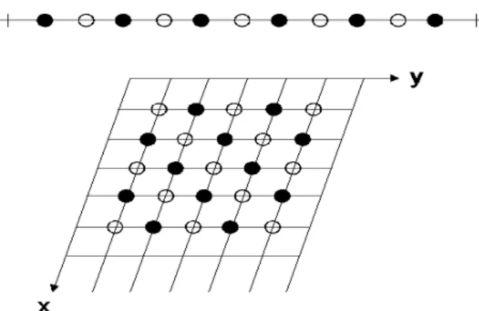
where sum of index i and j is odd. Fig. 1 shows red and black points. Red-black Gauss-Seidel has a clear advantage in terms of parallel computation.
Figure 1: A one-dimensional grid (top) and a two-dimensional grid (bottom) showing the
red points ◦ and the black points • for red-black relaxation.
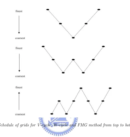
Two-grid correction is the basis of multigrid. Of course, we can repeat this process on successively coarser grids until arriving the coarsest grid. This is so-called V-cycle. To obtain more benefit from the coarser grids, where computations are cheaper, the W-cycle zigzags among the lower-level grids before moving back up to the finest grid. We can also join nested iteration idea which uses V-cycle on coarse grids to obtain improved initial guesses for fine grids. This is so-called full multigrid V-cycle (FMG).
The schedule of grids for V-cycle, W-cycle, and FMG show in Fig. 2. The complete algorithms of them are given in Algorithm 1,2,3 respectively. To describe Algorithm conveniently, we change some notations. We call the right-side vector of the residual equation f, rather than r, because it is just another right-side vector. Instead of calling the solution of the residual equation e, we use u because it is just a solution vector. We can then use v to denote approximations to u.
Algorithm 1 Vh(vh, fh) V-cycle Method
if (h=coarsest) then
vh = (Ah)−1fh {solve Ahuh = fh directly}
else
vh=Relax(vh, fh, ν
1) {pre-relax ν1 times with initial vh }
f2h= I2h
h (fh− Ahvh) {compute f2h by restricting residual}
v2h= 0
v2h= V2h(v2h, f2h) {V-cycle on the coarser grid }
vh = vh+ Ih
2hv2h {correct vh by interpolating v2h}
vh=Relax(vh, fh, ν
2) {post-relax ν2 times with modified vh }
Algorithm 2 Wh(vh, fh) W-cycle Method
if (h=coarsest) then
vh = (Ah)−1fh {solve Ahuh = fh directly}
else
vh=Relax(vh, fh, ν
1) {pre-relax ν1 times with initial vh }
f2h = I2h
h (fh− Ahvh) {compute f2h by restricting residual}
v2h = 0
v2h = V2h(v2h, f2h) 2 times {V-cycle on the coarser grid 2 times}
vh = vh+ Ih
2hv2h {correct vh by interpolating v2h}
vh=Relax(vh, fh, ν
2) {post-relax ν2 times with modified vh }
end if
Algorithm 3 F MGh(fh) Full Multigrid V-cycle Method
if (h=coarsest) then
vh = (Ah)−1fh {solve Ahuh = fh directly}
else
f2h= I2h
h (fh) {compute f2h by restricting fh}
v2h= F MG2h(f2h) {FMG on the coarser grid }
vh = Ih
2hv2h {compute vh by interpolating v2h}
vh = Vh(vh, fh) {V-cycle with modified vh }
end if
In this section, we have studied the elements of multigrid method. Although we don’t introduce all the details of multigrid method, we have enough ability to solve Helmholtz equations. [1] has complete introduction of multigrid method.
In brief, multigrid method integrate some easy ideas and schemes. In fact, these ideas may have some individual defects. Multigrid method arrange them skillfully such that they can work together, and result in a very useful numerical method.
Figure 2: Schedule of grids for V-cycle, W-cycle and FMG method from top to bottom.
3
Preconditioned Conjugate Gradient Method
The conjugate gradient method is one of the popular methods for solving linear system
Ax = b. It is very suitable for large-scale sparse matrices arising form FD or FE
approx-imation of boundary-value problems. When the n × n symmetric positive definite matrix has been preconditioned to make the calculations more effective, good results are obtain in only about √n steps.
In this section, we introduce roughly the conjugate gradient method, and its complete derivation can be found in [5].
First, we define the quadratic function
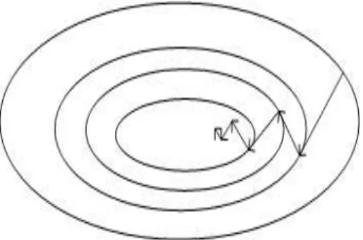
φ(x) = 1 2hAx, xi − hb, xi = 1 2x TAx − xTb, and let h(α) = φ(x + αs).
Figure 3: Convergence of steepest descent.
also find that h(α) has a minimal value when
α = hs, b − Axi hs, Asi
Now, we denote x an approximate solution to Ax∗ = b, and vector s 6= 0 gives a
search direction to improve the approximation. Let r = b − Ax be the residual vector associated with x and
α = hs, b − Axi hs, Asi =
hs, ri hs, Asi.
If r 6= 0 and if s and r are not orthogonal, then φ(x + αs) is smaller than φ(x) and x + αs is presumably closer to x∗ than x. This suggest the following method.
Let x0 be an initial approximation to x∗, and let s0 6= 0 be an initial search direction.
For k = 0, 1, 2, . . . , we compute αk = hsk, b − Axki hsk, Aski , xk+1 = xk+ αksk
and choose a new search direction sk+1. The object is to make this selection so that the
sequence of approximations {xk} converges rapidly to x∗.
Our direct idea is using −∇φ(x) as a search direction because it is the direction of greatest decrease in the value of φ(x). And it is just the direction of the residual r. The method that choose
sk+1 = rk+1 = b − Axk+1
is called the method of steepest descent. Unfortunately, the convergence rate of steepest descent is often very poor owing to repeated searches in the same directions (see Fig. 3). Therefore, the search direction requires some modifications not negative gradient direction any more. The conjugate gradient method chooses search directions {s0, . . . , sn−1} so that
they are A-orthogonal set; that is,
hsi, Asji = 0, if i 6= j.
Now, we use rk+1 to generate sk+1 by setting
sk+1 = rk+1+ βk+1sk.
We want to choose βk+1 so that
hsk, Ask+1i = 0. We can obtain βk+1 = − hsk, Ark+1i hsk, Aski .
It can be shown that with this choice of βk+1, {s0, . . . , sk+1} is an A-orthogonal set. Then
we can simplify αk = hrk, rki hsk, Aski . Thus, xk+1 = xk+ αksk.
To compute rk+1, we multiply by A and subtract b to obtain
rk+1 = rk− αkAsk.
Then we can change
βk+1 =
hrk+1, rk+1i
hrk, rki
.
Above derivation is the process of conjugate gradient method. The algorithm of conjugate gradient method is given in algorithm 4.
Algorithm 4 Conjugate Gradient Method x0 =initial guess
r0 = b − Ax0
s0 = r0
for k = 0, 1, 2, . . .
αk = rTkrk/sTkAsk {compute search parameter}
xk+1= xk+ αksk {update solution}
rk+1 = rk− αkAsk {compute new residual}
βk+1 = rTk+1rk+1/rTkrk
sk+1 = rk+1+ βk+1sk {compute new search direction}
conjugate gradient method can be accelerated by preconditioning. Preconditioning means that choose a matrix M for which systems of the form Mz = y are easily solved. And
M−1 ≈ A−1 so that M−1A is relatively well-conditioned. In fact, we should apply
con-jugate gradient to L−1AL−T instead of M−1A to preserve symmetry of matrix, where
M = LLT. However, the algorithm can be suitably rearrange so that only M is used and
the corresponding matrix L is not required explicitly. The algorithm of preconditioned conjugate gradient method is given in algorithm 5.
Algorithm 5 Preconditioned Conjugate Gradient Method x0 =initial guess
r0 = b − Ax0
s0 = M−1r0
for k = 0, 1, 2, . . .
αk = rTkM−1rk/sTkAsk {compute search parameter}
xk+1 = xk+ αksk {update solution}
rk+1 = rk− αkAsk {compute new residual}
βk+1 = rTk+1M−1rk+1/rTkM−1rk
sk+1 = M−1rk+1+ βk+1sk {compute new search direction}
end
Choosing an appropriate preconditioner is very important. The choice of precondi-tioner depends on the usual trade-off between the gain in the convergence rate and the increased cost per iteration that results from applying the preconditioner. Many types of preconditioner can be find in [6]. We only introduce some of them.
• Jacobi : M is taken to be a diagonal matrix with diagonal entries equal to those
of A. This is the easiest preconditioner since M−1 is also a diagonal matrix (can
be regarded as vector when we compute) whose entries are reciprocal of the diag-onal entries of A. Although it only increases less storage and cost per iteration, it need more number of necessary iterations than the following incomplete Cholesky factorization.
• Incomplete Cholesky factorization: Ideally, we can factor A into LLTby Cholesky
factorization, but this may incur unacceptable fill. We may instead compute an ap-proximate factorization A ≈ ˆL ˆLT that allows little or no fill (e. g. restricting the
nonzero entries of ˆL to be in the same positions as those of the lower triangle of A)
to save storage and CPU time, then use M = ˆL ˆLT as a preconditioner.
• Multigrid preconditioner : We choose directly M = A and find M−1r by
multi-grid method. This is so-called multimulti-grid conjugate gradient method (MGCG). This 10
method is also researched widely in many papers. We will use MGCG in the later numerical experiments.
Up to now, We have introduced MG and PCG. These methods belong to iterative method. In fact, fast direct methods have been developed for solving general poisson equation [9]. The following Concus and Golub method make a little modification to Helmholtz equation so that fast direct method can be used.
4
Concus and Golub Method
Concus and Golub propose an iterative scheme which uses fast direct solvers for the repeated solution of a Helmholtz problem [7]. Suppose original equation is
Ψu = −4u + g(x, y)u = f (x, y).
Concus and Golub provide a approach to utilize a modified form of the iterative procedure
−∆un+1= −∆un− τ (Ψun− f ),
where τ is a parameter. We use the shifted iteration
(−4 + K)un+1= (−4 + K)un− τ (Ψun− f ).
The discrete form is given by
(−4h+ KI)Vn+1= (−4h+ KI)Vn− τ [(−4h+ G)Vn− F )],
where K is a parameter, V is approximation to exact u, −4his a matrix from operator −4
discretization with mesh space h, G is a diagonal matrix with elements Gij = g(ih, jh),
F is a vector with elements Fij = f (ih, jh), and I is the identity matrix.
Now, we want to find spectral radius ρ for above iteration. We denote M ≡ −4h+
G operator, Φ is a vector, and νm,νM are the minimum and maximum eigenvalues of
eigenvalue problem MΦ = ν(−4h+ KI)Φ. To obtain it,
ρ(I − τ [−4h+ KI]−1M) = max{|1 − τ νm|, |1 − τ νM|}.
To estimate νm and νM, we use the Rayleigh quotient for ν,
ΦTMΦ ΦT(−4h+ KI)Φ = 1 + ΦT(G − KI)Φ ΦT(−4h+ KI)Φ then β − K β − K B − K B − K
where β and B are the minimal and maximal of function g(x, y),λm and λM are the
smallest and largest eigenvalue of −∆h, and K is between β and B.
In this, the Lemma in [7] help us finding the optimal choice of τ
τ = 2 νm+ νM = 2(λm+ K) (2λm+ B + β) therefore ρ ≤ B − β 2λm+ B + β .
We will use this formula to observe the convergence rate of Concus and Golub method in the later numerical examples.
In an attempt to make the operator −4 + K on the left-hand side agree closely with Ψ, we usually set K the so-called min-max value,
1
2(min(g(x, y)) + max(g(x, y)))
so the optimal τ = 1. And then, the shifted iteration formula can be simplified
(−4h+ KI)Vn+1= (KI − G)Vn+ F.
According to above discrete form, we give an initial guess first, and compute right-hand side. Now, we can solve “Poisson equation” by FPS to gain the approximation and then update right-hand side again. Repeat this action until it reaches stopping criterion.
In fact, K can also be optimized for higher rates of convergence. The efficiency of Concus and Golub’s method can be increased by extending its formulation to accommo-date the use of a parameter K which is a one-dimensional function instead of a constant [7]. Unfortunately, for a special solution, that would have required a prohibitively large computational time since there is no fast Helmholtz solver available for variable coefficient. In the past it has been demonstrated that the number of necessary iterations can vary dramatically, depending on the function g(x, y) which has a critical role on the rate of convergence. The smoother g(x, y) is, the faster rate of convergence. We will give a example in the next section.
5
Numerical Examples
We will solve Helmholtz equations with Dirichlet boundary condition
−4u(x, y) + g(x, y)u = f (x, y), (x, y) ∈ Ω (3)
u(x, y) = p(x, y), (x, y) ∈ ∂Ω on domain Ω = [−1, 1] × [−1, 1].
First, we use five-point finite difference formula to discretize e.q. (3). Assume domain is partitioned into n × n subdomain by introducing the grid points
xi = ih, yj = jh, 0 ≤ i, j ≤ n
, where h = 2
n is the uniform mesh size.
We denote
vij : as an approximation to the exact solution u(xi, yj)
Fij : as the value of f (x, y) at (xi, yj)
Gij : as the value of g(x, y) at (xi, yj)
Pij : as the value of p(x, y) at (xi, yj).
Then, we can obtain discrete component form
−1
h2 (vi−1,j + vi+1,j+ vi,j−1+ vi,j+1− 4vij) + Gijvij = Fij,
and we can use iterative method to improve approximation vij according to
vij =
1
4 + h2Gij(vi−1,j+ vi+1,j + vi,j−1+ vi,j+1+ h 2F ij), for i = 1, ..., n − 1, j = 1, ..., n − 1 with v0j = P0j, vnj = Pnj, for j = 0, ..., n and vi0= Pi0, vin = Pin, for i = 0, ..., n.
We may also represent system in matrix form as Av = b.
A is an (n − 1) × (n − 1) block matrix, T is an (n − 1) × (n − 1) matrix and I is the
identity matrix of order n − 1.
A = 1 h2 T1 I I T2 I . .. ... ... I Tn−2 I I Tn−1 , Tj = 4 + h2G 1j −1 −1 4 + h2G 2j −1 . .. . .. . .. −1 4 + h2G −1 .
And the unknown vector v is defined by v = v1 v2 ... vn−2 vn−1 , vj = v1j v2j ... v(n−2),j v(n−1),j .
And the right-hand side vector b is defined by
b = b1 b2 ... bn−2 bn−1 , bj = b1j b2j ... b(n−2),j b(n−1),j . Then set bij = F ij, for i, j = 2, ..., n − 2 b1j = F1j+ P0j/h2, bn−1,j = Fn−1,j+ Pnj/h2, for j = 2, ..., n − 2
bi1= Fi1+ Pi0/h2, bi,n−1 = Fi,n−1+ Pi,n/h2, for i = 2, ..., n − 2
and
b1,1 = F1,1+ P0,1/h2+ P1,0/h2, bn−1,1 = Fn−1,1+ Pn−1,0/h2+ Pn,1/h2
b1,n−1= F1,n−1+ P0,n−1/h2+ P1,n/h2, bn−1,n−1 = Fn−1,n−1+ Pn−1,n/h2+ Pn,n−1/h2.
Our stopping criterion is krkh
kbkh
< 10−8, where r = b − Av is residual, and k • k
h means
discrete L2 norm.
We use the following methods for solving later examples.
• Concus and Golub method: Choose K equal to min-max value, and use
“GEN-BUN” routine which is in “FISHPACK” as our fast poisson solver.
• V-cycle method: Use RBGS relaxation with 2 sweeps before the correction step
and 1 sweep after the correction step. And use full weighting restriction and linear interpolation operators.
• ICCG method: Use Incomplete Cholesky factorization as a preconditioner of
con-jugate gradient method.
• MGCG method: Use V-cycle method as a preconditioner of conjugate gradient
method.
We choose two coefficient functions gs(x, y) = − sin(π(x + y)) 3 2 + sin(π(x + y)) and go(x, y) = − 80 sin(2π(x + y)) 3 2 + sin(2π(x + y)) .
Clearly, gs(x, y) is a smoother function. The maximum of gs(x, y) is about equal to 2.0,
and the minimum of gs(x, y) is about equal to −4.0 on the domain [−1, 1]×[−1, 1]. On the
contrary, go(x, y) is a large amplitude function. The maximum and minimum of go(x, y)
are 160 and −32 respectively. We also choose two functions
us(x, y) = sin(πx) + cos(πy)
and
uo(x, y) = (y2− 1)(y − 1)(e5ysin(4πx) + e−5ycos(4πx))
as our exact solutions. The function us(x, y) is smoother than uo(x, y). This also means
that the approximation of us(x, y) is more accurate than the approximation of uo(x, y)
under the same conditions.
Now, we use these functions gs(x, y), go(x, y), us(x, y) and uo(x, y) to result four
examples, and show numerical results including CPU time (sec.) and necessary iterations to achieve stopping criterion on different grid numbers N = 1282, 2562, 5122, 10242.
Example 1.1: gs(x, y) uo(x, y)
Iterations Concus and Golub ICCG MGCG V-cycle
N = 1282 5 117 7 7
N = 2562 5 218 7 7
N = 5122 5 428 7 6
N = 10242 5 796 7 6
CPU time Concus and Golub ICCG MGCG V-cycle
N = 1282 0.3 0.7 0.6 0.6
N = 2562 1.1 4.6 2.3 2.2
N = 5122 4.8 34.0 9.2 7.8
N = 10242 23.0 264.0 36.6 31.0
In this example, we can find that ICCG is not a good method since it need longer CPU time to achieve stopping criterion. So incomplete Cholesky factorization is not a good
Cholesky factorization (MIC) for construction of the preconditioning matrix, see [6]. We
also find that the number of iterations of ICCG increases when N becomes larger. The other methods like Concus and Golub, MGCG, V-cycle converge with very few iterations. And their number of iterations is almost independent of N. Therefore, the CPU time needed for these methods reach stopping criterion is much less than ICCG when N is very large.
Up to now, Concus and Golub method seem to converge rapidly. It is even better than multigrid method. Let us continue seeing the next example.
Example 1.2: go(x, y) uo(x, y)
Iterations Concus and Golub ICCG MGCG V-cycle
N = 1282 271 144 9 11
N = 2562 267 282 9 10
N = 5122 266 533 9 9
N = 10242 266 1006 9 8
CPU time Concus and Golub ICCG MGCG V-cycle
N = 1282 9.0 0.73 0.7 0.8
N = 2562 36.0 5.2 2.8 3.0
N = 5122 158.0 39.0 11.6 10.8
N = 10242 784.0 305.0 46.0 40.0
This example uses a high amplitude function go(x, y) as coefficient. Clearly, the iterations
and CPU time of all methods increase. But we note that Concus and Golub method results in very very slow convergence. Its CPU time needed is even longer than ICCG. This phenomenon can be explained by below inequality introduced in the last section.
ρ ≤ M − m
2λ + M + m < 1,
where M and m denote the maximum and minimum of g(x, y) respectively. λ is the smallest eigenvalue of the discrete matrix of Laplace operator, and ρ is the spectral radius of iterative matrix of Concus and Golub method. In example 1.1
M − m
2λ + M + m ≈ 0.08,
but in example 1.2
M − m
2λ + M + m ≈ 0.93.
That is why Concus and Golub method need so many iterations to reach stopping criterion here. In next two examples 2.1,2.2 we replace uo(x, y) in examples 1.1,1.2 with us(x, y).
Example 2.1: gs(x, y) us(x, y)
Iterations Concus and Golub ICCG MGCG V-cycle
N = 1282 9 124 7 7
N = 2562 9 232 7 6
N = 5122 9 442 7 6
N = 10242 9 869 6 6
CPU time Concus and Golub ICCG MGCG V-cycle
N = 1282 0.3 0.6 0.5 0.5
N = 2562 1.3 4.1 1.9 1.6
N = 5122 5.6 30.6 7.8 6.4
N = 10242 28.3 257.0 27.3 25.6
Example 2.2: go(x, y) us(x, y)
Iterations Concus and Golub ICCG MGCG V-cycle
N = 1282 394 144 9 12
N = 2562 393 282 9 10
N = 5122 392 554 9 10
N = 10242 392 1078 9 8
CPU time Concus and Golub ICCG MGCG V-cycle
N = 1282 12.0 0.63 0.6 0.8
N = 2562 53.0 4.9 2.6 2.6
N = 5122 228.0 38.0 10.2 10.6
N = 10242 1153.0 317.0 41.0 35.0
After observing results of these two examples, we get the same conclusion discussed before. But we can find another phenomenon by comparing with example 1.1 and example 1.2. The number of iterations and CPU time needed of Concus and Golub method and ICCG increase, but MGCG and V-cycle almost remain the same number of iterations even if us(x, y) may cause smoother error in these examples. That is because multigrid
method can reduce smooth error efficiently.
In this thesis, we do not compare MGCG and V-cycle (ordinary multigrid) methods. Which is the better method? What is the difference of behaviors between the MCCG and multigrid methods? We can find answer in [10]. In [10], it gives a special example. The matrix produced by the discretization of this example has scattered eigenvalues. This scattered eigenvalues prevent the ordinary multigrid method from converging rapidly. We can observe the eigenvalue’s distribution after multigrid preconditioning from [10]. Almost all eigenvalues are clustered, and a few eigenvalues are scattered. The conjugate gradient method hides the defect of the multigrid method. Therefore, the MGCG method
6
Conclusion
After testing above examples, we know that multigrid method suits to be used for solving general nonseparable elliptic equations. Since no matter g(x, y) is smooth or oscillatory and smooth or oscillatory error resulted, multigrid method always converges in very few iterations. This means that multigrid method convergence stably. We also know an important advantage of multigrid method from our nu- merical examples. That is the number of necessary iterations is independent of mesh size.
There is another advantage of multigrid method. It is easy to be parallelized. We do not introduce the parallelism of multigrid method in this thesis. The content of parallel multigrid can be studied from [11]. These above reasons explain why we use multigrid method for solving Helmholtz equation here.
References
[1] William L. Briggs Van Emden Henson Steve F. McCormick, A multigrid toturial 2nd
ed. 2000.
[2] A. BRANDT, Multigrid Techniques: 1984 Guide with Applications to Fluid
Dynam-ics, GMD-Studien Nr. 85, Gesellschaft f¨ur Mathematik und Datenverarbeitung, St.
Augustin, Bonn, 1984.
[3] Michael T. Heath, Scientific computing :an introductory survey 2nd ed. 2002.
[4] W. M. Pickering and P. J. Harley , Numerical solution of non-separable elliptic
equa-tions by iterative application of FFT methods. Int. Jnl. Computer Math. 55, 211-222,
1995.
[5] Richard L. Burden, J. Douglas Faires, Numerical analysis 7th ed. 2001. [6] Yousef Saad, Iterative methods for sparse linear systems, 1996.
[7] Paul Concus and Gene H. Golub, Use of fast direct met hods for the efficient
nu-merical solution of nonseparable elliptic equations, SIAM J. Numer. Anal. 10 pp.
1103-1120, 1973.
[8] Dimitropoulos, C.D. and Beris, A.N. An efficient and robust spectral solver for
non-separable elliptic equations J. Comp. Phys. 133 pp. 186-191, 1997.
[9] B. Buzbee, G. Golub, and C. Nielson, On direct methods for solving Poissons
equa-tion, SIAM J. Numer. Anal. 7 pp. 627-656, 1970.
[10] Osamu Tatebe, The multigrid preconditioned conjugate gradient method [11] Jim E. Jones, A Parallel Multigrid tutorial.