多頻正交分頻多工系統同步之研究

全文

(1)國立交通大學電子工程系碩士論文. 多頻正交分頻多工系統同步之研究 A Study of Synchronization in MB-OFDM UWB Systems. 研究生：王景文指導教授：桑梓賢. 教授. 中華民國九十四年六月.

(2) 多頻正交分頻多工系統同步之研究 A Study of Synchronization in MB-OFDM UWB Systems. 研究生：王景文. Student：Wang Chin-Wen. 指導教授：桑梓賢. Advisor：Sang Tzu-Hsien. 國立交通大學電子工程學系碩士論文. A Thesis Submitted to Department of Electronic Engineering College of Electrical Engineering and Computer Science National Chiao Tung University in partial Fulfillment of the Requirements for the Degree of Master in. Electronic Engineering June 2005 Hsinchu, Taiwan, Republic of China. 中華民國九十四年六月.

(3) 多. 頻. 正. 交. 分. 頻. 多. 工. 系. 統. 同. 學生：王景文. 步. 之. 研. 究. 指導教授：桑梓賢. 國立交通大學電子工程學系﹙研究所﹚碩士班. 摘. 要. 多頻正交分頻多工系統 (MB-OFDM) 為一種利用跳頻展頻(FHSS)將 OFDM 訊號頻寬展開的超寬頻 (Ultra-wide band) 系統。然而因其為慢跳頻 ( slow frequency hopping) 及有限的可跳頻頻帶，在多個子網路 (piconet) 時，其頻帶可能因交錯而互相干擾，因此在設計 MB-OFDM 接收機時，其對共頻帶干擾的強健性為一重要的課題。. 本論文提出一個對干擾具有高強健性的封包偵測架構。此架構是利用一匹配濾波器 (match filter)，對輸入信號與封包頭的訓練序列(training sequence)進行匹配濾波。並利用訓練序列的週期性，將匹配濾波器的輸出進行延遲相關 (delay correlate)運算而達成高強健性的目的。本論文同時提出對其他的同步問題作出討論，並提出一可行的同步程序。. i.

(4) A Study of Synchronization in MB-OFDM UWB Systems. student：Wang Chin-Wen. Advisors：Dr.Sang. Tzu-Hsien. Department﹙Institute﹚of Electronic Engineering National Chiao Tung University. ABSTRACT. Multi-band orthogonal frequency-division multiplexing (MB-OFDM) is an UWB modulation technique which combines OFDM and frequency hopping spread spectrum (FHSS) to archive high data rate and low interference to other communication systems. Due to its slow-hopping pattern, OFDM technology and the limited number of frequency bands available, when geographically overlapped multiple piconets are considered, there is no coordination of transmissions among different piconets. The robustness to interference is thus an important issue for MB-OFDM systems.. This thesis provides a packet detection scheme which is robust to the interference of simultaneous operating piconets (SOP). This scheme makes use of a match filter (MF) to match the preamble, and a delay correlator is utilized to take advantage of the periodicity of MB-OFDM preamble. This thesis also discuss other synchronization issues like carrier frequency offset and sampling clock offset for MB-OFDM system.. ii.

(5) 誌. 謝. 這篇論文的完成，首先要感謝我的指導教授，桑梓賢老師，其亦師亦友的指導方式與對學生充份信任且自由開放的引導方向，使我們受益匪淺。再來很重要的，必須感謝我父母，劉新春女士及王茂萱先生，的養育之恩與無私的愛，雖然他們來不及看到我順利畢業，然希望這篇論文的付梓，能夠榮耀他們。感謝我的家人們，雖然他們都有其事業要忙，然而在適當的時候總能團結起來。並給于我奧援。室驗室的同學與學弟們，謝謝你們能夠容忍我的個性，讓這兩年的研究生活愉快而充實。然而要感謝的人太多，或許有所遺漏，也望能見諒。. iii.

(6) Table of Content Table of Content................................................................................................... iv List of Figures....................................................................................................... v List of Tables ....................................................................................................... vii Chapter 1. Introduction...................................................................................... 1. Chapter 2 Introduction of MB-OFDM proposal................................................. 3 2.1 Introduction to MB-OFDM architecture................................................. 3 2.2 Frame structure........................................................................................ 11 2.3 Interference of MB-OFDM system......................................................... 21 2.4 UWB Channel Model............................................................................... 22 Chapter 3 Packet detection and some timing synchronization issues.............. 28 3.1 introductions to synchronization tasks .................................................. 28 3.2 Packet detection basic issues ................................................................... 28 3.3 MF with delay correlator ........................................................................ 36 3.4 The two comparator scheme ................................................................... 43 3.5 The Timing issues..................................................................................... 52 Chapter 4. Other MB-OFDM synchronization issues .................................... 54. 4.1 Carrier frequency offset (CFO) and timing offset effect in MB-OFDM system .............................................................................................................. 54 4.2 The synchronization strategy.................................................................. 59 Chapter 5. Conclusion and future research suggestion.................................. 64. Reference ............................................................................................................ 65 Appendix MB-OFDM preamble ........................................................................ 66. iv.

(7) List of Figures figure 2.1.1 piconet elements (source : 802.15.3 standard) ................. 3 figure 2.1.2 input and output of IFFT...................................................... 4 figure 2.1.3 subcarrier frequency allocation (source : 802.15.3a proposal ) ......................................................................................... 5 figure 2.1.4 transmit power spectrum density mask................................ 9 figure 2.1.5 The overlap adding of received signal............................... 11 figure 2.2.3 CCITT CRC-16 implement (source : 802.15.3a proposal) 15 figure 2.2.5 11/32 coding rate bit-stealing and bit-insertion procedure (source : 802.15.3a proposal) ........................................................ 18 figure 2.2.6 1/2 coding rate bit-stealing and bit-insertion procedure (source : 802.15.3a proposal) ........................................................ 18 figure 2.2.7 5/8 coding rate bit-stealing and bit-insertion procedure (source : 802.15.3a proposal) ........................................................ 19 figure 2.2.8 3/4 coding rate bit-stealing and bit-insertion procedure ...... (source : 802.15.3a proposal) 19 figure 2.2.9 QPSK constellation bit encoding (source : 802.15.3a proposal) ........................................................................................ 20 figure 2.2.10 802.15.3a packet forming procedure .......................... 21 figure 2.3.1 SOP collision situation....................................................... 22 figure 2.4.1 Multipath of MB-OFDM ................................................ 23 figure 3.2.2 MF structure.................................................................... 30 figure 3.2.3 PSD of MB-OFDM symbol............................................... 31 figure 3.2.4 Autocorrelation of MB-OFDM symbol.......................... 32 figure 3.2.5 SOP simulation model .................................................... 33 figure 3.2.6 The PDF of MF output....................................................... 35 figure 3.2.7 FAR/Missing rate versus SNR of MF scheme................... 36 figure 3.2.8 FAR/Missing rate versus threshold of MF scheme ........... 36 figure 3.3.1 delay correlator scheme .................................................. 37 figure 3.3.2 PDF of the product of two Gaussian r.v. with bias ......... 39 figure 3.3.2 CDF of the product of two Gaussian r.v. with bias......... 40 figure 3.3.4 FAR/Missing versus threshold of delay correlator scheme40 figure 3.3.5 FAR/Missing versus SNR of delay correlator scheme ... 42 figure 3.3.6 The cross-correlation degradation due to CFO.................. 42 figure 3.4.2 FAR versus threshold of two comparator scheme ........ 46 figure 3.4.3 Miss rate versus threshold of two comparator scheme. 46 figure 3.4.4 FAR/Miss rate versus SNR of two comparator scheme .... 47 figure 3.4.5 The modified version of 2 comparator scheme .............. 48 figure 3.4.6 FAR versus thresholds of modified two comparator scheme ........................................................................................... 50 figure 3.4.6 miss rate versus thresholds of modified two comparator scheme ........................................................................................... 50 v.

(8) figure 3.4.7 FAR/Miss rate versus SNR of modified two comparator scheme ........................................................................................... 51 figure 3.5.1 Composite of an OFDM symbol........................................ 52 figure 3.5.2 The relationship between received signal and MF output ....................................................................................................... 53 figure 4.1.2 SNR degradation versus Es/N0 due to CFO ....................... 55 figure 4.1.4 The SNR degradation due to sampling frequency offset versus Es/N0 ................................................................................... 58 figure 4.1.5 Rotation due to SFO and CFO versus tone index........... 59 figure 4.2.1 Synchronization flowchart ................................................. 60 figure 4.2.2 Phase rotation ambiguity due to CFS and sampling frequency offset ............................................................................. 63 figure A-1 the cross-correlation of the preambles with time shift......... 66. vi.

(9) List of Tables Table 2.1.1 Time relative parameters of MB-OFDM.............................. 5 Table 2.1.2 Rate-dependent parameters .................................................. 7 Table 2.1.3 OFDM PHY band allocation ................................................ 8 Table 2.1.4 time frequency code............................................................ 10 Table 2.2.5 Rate-dependent parameters ............................................. 14 Table 2.2.6 Scramble seed selection...................................................... 16 Table 2.4.1 channel model parameters ............................................... 27 Table A-1 – Time-domain packet synchronization sequence for Preamble Pattern 1......................................................................... 67 Table A-2 – Time-domain packet synchronization sequence for Preamble Pattern 2......................................................................... 68 Table A-3 – Time-domain packet synchronization sequence for Preamble Pattern 3......................................................................... 69 Table A-4 – Time-domain packet synchronization sequence for Preamble Pattern 4......................................................................... 70. vii.

(10)

(11) Chapter 1. Introduction. By the FCC’s (U.S. Federal Communications Commission) definition, UWB communication systems use signals with -10dB fractional bandwidth that is larger than 20% of the center frequency, or greater than 500 MHz. Besides, FCC gives the rigid spectrum mask which the power spectrum density of the UWB signal should be within. With the low power spectrum density of UWB systems, the UWB signals could be regarded as noise by other narrow-band services. On the other hand, with the wide PSD, the disturbance of narrow-band signal occupies only a small fraction of the total bandwidth, and the data corrupted by narrow-band interference could be recovered with FEC.. Traditional UWB communication systems, named impulse-radio UWB, use the signal of ultra-short, low duty cycle pulses, and is transmitted without carrier. Due to the difficulty of controlling the shape of the pulse, such systems tend to use all of the bandwidth, and sometimes it is called single-band system. The new FCC regulations that allow UWB signal transmitted in the range of 3.1GHz to 10.6 GHz. The carrier-based UWB systems generating signals using techniques to spread spectrum based on either single-carrier or multi-carrier or both of them. Single-carrier UWB could be viewed as a spread spectrum system whose signal bandwidth is spread ultra wide. Different multi-carrier ultra wideband (MC-UWB) systems have been recently proposed for high bit rate wireless networks in dense multi-path fading channels. One of the multi-carrier UWB systems is Multiband-OFDM that uses a frequency hopping scheme for reliable bit rate communication over multi-path fading channel. 1.

(12) OFDM concept was first proposed in 1966[1] for dispersive fading channels, but is not mature until 1990s. It cuts a band into several sub-bands where QAM symbols map into, and overlaps these sub-bands efficiently. That makes the synchronization accuracy in timing or carrier frequency of OFDM receivers critical. There exist lots of algorithms which try to solve those problems. Based on the MB-OFDM proposal, the system contains OFDM and frequency hopping technology. The frequency hopping system has its own timing synchronization, so the synchronization issues should be taken care simultaneously. This thesis discusses about these issues and tries to provide a solution.. The thesis is organized as follows: Chapter 2 gives the introduction to MB-OFDM proposal of MBOA. Chapter 3 will discuss and analyze the issues of packet detection and some timing synchronization problems. Chapter 4 will discuss other MB-OFDM synchronization issues like frequency and timing offset estimation and compensation. And Chapter 5 will give a conclusion.. 2.

(13) Chapter 2 Introduction of MB-OFDM proposal. 2.1 Introduction to MB-OFDM architecture In this section a brief introduction of an UWB system intended for wireless personal area network (WPAN) is presented. It uses the modulation based on MB-OFDM for conveying information over relatively short distances among few participants. Every device of the communication system interacts using the concept of piconets. A piconet is a wireless ad hoc data communications system which allows a number of independent data devices (DEVs) to communicate with each other. An 802.15.3a piconet consists of several components, as shown in figure 2.1.1. The basic component is the DEV. One DEV is required to assume the role of the piconet coordinator (PNC) of the piconet. The PNC provides the basic timing for the piconet with the beacon. Additionally, the PNC manages the quality of service (QoS) requirements, power save modes and access control to the piconet.. figure 2.1.1 piconet elements (source : 802.15.3 standard) .. 3.

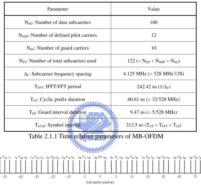
(14) WPAN is a packet base transmitting communication system. A packet is composed with couples of OFDM symbol. It uniformly cuts 528 MHz to 128 subcarriers, 4.125 MHz for each subcarrier, in which 100 subcarriers are for information tones, 12 subcarriers are for pilot tones, 10 subcarriers are for guard tones, and 6 subcarriers are for null tones. The relative location in frequency domain is shown in figure 2.1.3. The time and frequency domain transform is implemented using Fast Fourier Transform/ Inverse Fourier Transform (FFT/IFFT) (figure 2.1.2), and the FFT/IFFT period is 242.42 ns. In each OFDM symbol, there are 32 sampling intervals for cyclic prefix extension and 5 sampling intervals for guard intervals which are used for frequency hopping. So it takes 312.5 ns to transmit an OFDM symbol. The relative parameters are summarized in table 2.1.1.. figure 2.1.2 input and output of IFFT. 4.

(15) Parameter. Value. NSD: Number of data subcarriers. 100. NSDP: Number of defined pilot carriers. 12. NSG: Number of guard carriers. 10. NST: Number of total subcarriers used. 122 (= NSD + NSDP + NSG). ∆F: Subcarrier frequency spacing. 4.125 MHz (= 528 MHz/128). TFFT: IFFT/FFT period. 242.42 ns (1/∆F). TCP: Cyclic prefix duration. 60.61 ns (= 32/528 MHz). TGI: Guard interval duration. 9.47 ns (= 5/528 MHz). TSYM: Symbol interval. 312.5 ns (TCP + TFFT + TGI). Table 2.1.1 Time relative parameters of MB-OFDM. figure 2.1.3 subcarrier frequency allocation (source : 802.15.3a proposal ). In each OFDM symbol, twelve pilot signals are for the purpose of making coherent detection robust against frequency offsets and phase noise. These pilot signals shall be put in subcarriers numbered –55, –45, –35, –25, –15 –5, 5, 15, 25, 35, 45, and 55. The contribution due to the pilot subcarriers for the kth OFDM symbol is given by the inverse Fourier Transform of the sequence Pn below, which is further BPSK modulated by a pseudo-random binary sequence, 5.

(16) pl (defined further below), to prevent the generation of spectral lines. ⎧1 + j ⎪ 2 ⎪ Pn = ⎪⎨ − 1 − j ⎪ 2 ⎪0 ⎪⎩. n = 15,45 n = 5,25,35,55 n = ±1...,±4, ,±6,...,±14,±16,...,±24,±26,...,±34,±36,...,±44,±46,...,±54,±56. For modes with data rates less than 106.67 Mbps: Pn ,k = P−*n ,k ,. n = −5,−15,−25,−35,−45,−55. For 106.67 Mbps and all higher rate modes: Pn ,k = P− n ,k ,. n = −5,−15,−25,−35,−45,−55. The polarity of the pilot subcarriers is controlled by the following pseudo-random LFSR sequence, pl: p0…126 = {1, 1, 1, 1, -1, -1, -1, 1, -1, -1, -1, -1, 1, 1, -1, 1, -1, -1, 1, 1, -1, 1, 1, -1, 1, 1, 1, 1, 1, 1, -1, 1, 1, 1, -1, 1, 1, -1, -1, 1, 1, 1, -1, 1, -1, -1, -1, 1, -1, 1, -1, -1, 1, -1, -1, 1, 1, 1, 1, 1, -1, -1, 1, 1, -1, -1, 1, -1, 1, -1, 1, 1, -1, -1, -1, 1, 1, -1, -1, -1, -1, 1, -1, -1, 1, -1, 1, 1, 1, 1, -1, 1, -1, 1, -1, 1, -1, -1, -1, -1, -1, 1, -1, 1, 1, -1, 1, -1, 1, 1, 1, -1, -1, 1, -1, -1, -1, 1, 1, 1, -1, -1, -1, -1, -1, -1, -1}. MB-OFDM WPAN provides 53.3, 80, 110, 160, 200, 320, 400, and 480 Mb/s data rates. Unlike 802.11a, those rates are archived by changing the coding rate of convolutional code and the spreading factors instead of by modulation. The modulation used in this proposal is only QPSK. The relative between the data rate and the parameters is as shown in table 2.1.2. Where the conjugate symmetric input to IFFT means that data is just carried by the tone with positive index, and the tones with negative index take the values conjugate to that of 6.

(17) positive indexes symmetrically. And the time spreading is implemented by transmitting the same OFDM twice.. Coding. Conjugate. Time. Overall. Coded bits. Rate. rate. Symmetric. Spreading. Spreading. per OFDM. (Mb/s). (R). Input to. Factor. Gain. symbol. Data. Modulation. (NCBPS). IFFT 53.3. QPSK. 1/3. Yes. 2. 4. 100. 80. QPSK. ½. Yes. 2. 4. 100. 110. QPSK. 11/32. No. 2. 2. 200. 160. QPSK. ½. No. 2. 2. 200. 200. QPSK. 5/8. No. 2. 2. 200. 320. QPSK. ½. No. 1 (No. 1. 200. 1. 200. 1. 200. spreading) 400. QPSK. 5/8. No. 1 (No spreading). 480. QPSK. ¾. No. 1 (No spreading). Table 2.1.2 Rate-dependent parameters. The WPAN PHY operates in 3.1 – 10.6 GHz frequency as regulated by FCC. The relation between center frequency and band number is given by the equation: Band center frequency = 2904 + 528 × nb , nb = 1...14 (MHz). Based on this definition, five band groups are defined, consisting four groups of tree bands each and one group of two bands. Band group 1 is used for Mode 1 devices (mandatory mode). The remaining band groups are reserved for future use. The band allocation is summarized in table 2.1.3. The transmitted signal power in each band is limited by the power spectrum density (PSD) mask (figure 2.1.4) regulated by FCC. 7.

(18) Band Group. BAND_ID. Lower frequency. Center frequency. Upper frequency. 1. 1. 3168 MHz. 3432 MHz. 3696 MHz. 2. 3696 MHz. 3960 MHz. 4224 MHz. 3. 4224 MHz. 4488 MHz. 4752 MHz. 4. 4752 MHz. 5016 MHz. 5280 MHz. 5. 5280 MHz. 5544 MHz. 5808 MHz. 6. 5808 MHz. 6072 MHz. 6336 MHz. 7. 6336 MHz. 6600 MHz. 6864 MHz. 8. 6864 MHz. 7128 MHz. 7392 MHz. 9. 7392 MHz. 7656 MHz. 7920 MHz. 10. 7920 MHz. 8184 MHz. 8448 MHz. 11. 8448 MHz. 8712 MHz. 8976 MHz. 12. 8976 MHz. 9240 MHz. 9504 MHz. 13. 9504 MHz. 9768 MHz. 10032 MHz. 14. 10032 MHz. 10296 MHz. 10560 MHz. 2. 3. 4. 5. Table 2.1.3 OFDM PHY band allocation. 8.

(19) figure 2.1.4 transmit power spectrum density mask. In 802.15.3a standard, the maximum center frequency offset (CFO) of transmitter and receiver is ±20ppm. In operation mode 1, operated with center frequency 4488 MHz and relative oscillator offset is ±40ppm, the maximum CFO sensed by receiver is 0.17952 MHz ( about 0.04 of the distance between subcarriers).. MB-OFDM preamble composed of tree kinds of training sequence: (1) packet synchronization sequence (defined in time domain), (2) frame synchronization sequence (defined in time domain), and (3) channel estimation sequence (defined in frequency domain).. Unique logical channels corresponding to different piconets are defined by using up to four different time-frequency codes for each band group. Different preamble patterns are used in conjunction with the different time-frequency 9.

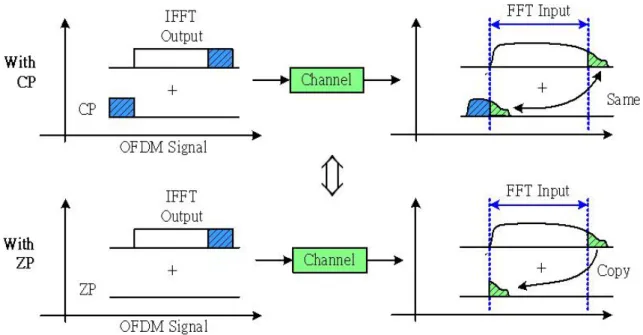
(20) codes. The time-frequency codes and associated preamble patterns for Mode 1 devices (which operate in band group 1) are defined in table 2.1.4.. Channel Preamble. Mode 1: Length 6 Time. Number. Pattern. Frequency Code. 1. 1. 1. 2. 3. 1. 2. 3. 2. 2. 1. 3. 2. 1. 3. 2. 3. 3. 1. 1. 2. 2. 3. 3. 4. 4. 1. 1. 3. 3. 2. 2. 5. 1. 1. 2. 1. 2. 1. 2. 6. 2. 1. 1. 1. 2. 2. 2. Table 2.1.4 time frequency code. MB-OFDM use zero padding instead of cyclic extension. The reason for using zero padding is that adding cyclic extension in an OFDM symbol makes the autocorrection of the sequence raise high at specific moment. PSD is the fourier transform of autocorrection function, and the raising of autocorrection function makes the PSD of the transmitted signal ripple. Zero padding has no such problem, and it also provides the same robustness to multipath fading as cyclic extension. But a little modification should be made in order to eliminate the inter-carrier interference due to the inaccuracy of symbol timing. The modification name “overlap adding” is adding the signal spreading from the FFT input to the front part of the signal (figure 2.1.5). This modification makes the zero-padding signal looks like the cyclic prefix one.. 10.

(21) figure 2.1.5 The overlap adding of received signal. 2.2 Frame structure 802.15.3a is a packet base transmitting communication system. The structure of this packet is shown in figure 2.2.1. figure 2.2.1 PLCP frame format (source : 802.15.3a proposal). Three sections are contained in a complete PLCP frame: 1. PLCP preamble 2. PLCP header 3. Data 11.

(22) A PLCP preamble is added prior to the PLCP header to aid receiver algorithms related to synchronization, CFO recovery, and channel estimation. Two portions, the time domain packet and frame synchronization sequence for total 24 or 12 OFDM symbol durations long, and the frequency domain channel estimation sequences compose the PLCP preamble for 6 OFDM symbol durations long.. There are four packet synchronization patterns defined (see appendix). Each time domain preamble is decided by the four patterns and cover sequence pc(n) (of length 24 for standard preamble) ,the table is in the appendix, and the combined packet and frame synchronization portion are generated as the Kronecker product of the two sequences. In additional to standard preamble, a shorten preamble is also defined for use in the streaming mode when a burst of packet is transmitted, separated by a MIFS time. For data rates of 200 Mbps and lower, all the packets in the burst mode use the standard PLCP preamble. However, for data rates higher than 200 Mbps, the first packet uses the standard preamble, while the remaining packets may use the shorten preamble. This portion of the preamble can be used for packet detection and acquisition, coarse carrier frequency estimation, and coarse symbol timing. As for the channel estimation portion, the training sequence is generated by passing the frequency-domain sequence defined in table 2.2.1 through the IFFT, and appending a zero pad interval consisting of 37 zeros to the resulting time-domain output. This portion of the preamble can be used for estimation of the channel frequency response, fine CFO estimation, and fine symbol timing.. The OFDM training symbols shall be followed by the PHY header, which 12.

(23) contains the RATE of the MAC frame body, the length of the frame payload (which does not include the FCS), the seed identifier for the data scrambler, and information about the next packet-whether it is being sent in streaming mode and whether it employs a shortened preamble or not. The RATE field conveys the information about the type of modulation, the coding rate, and the spreading factor used to transmit the MAC frame body.. The PHY header field shall be composed of 40 bits, as illustrated in figure 2.2.2. Bits 3-7 encode the RATE, as shown in table 2.2.5. Bits 8–19 encode the LENGTH field, with the least significant bit (LSB) being transmitted first. Bits 22–23 encode the seed value for the initial state of the scrambler, which is used to synchronize the descrambler of the receiver. Bit 26 encodes whether the packet is being transmitted in “burst” or streaming mode. In burst mode, the minimum packet size shall be 1 byte. In non-burst mode, the minimum packet size should be zero byte. Bit 27 encodes the preamble type (set to 0 for long or 1 for short preamble) used in the next packet if in streaming mode. All other bits are reserved for future use and are set to zero.. figure 2.2.2 PHY header bit assignment (source : 802.15.3a proposal). 13.

(24) Rate (Mb/s). R1 – R5. 53.3. 00000. 80. 00001. 110. 00010. 160. 00011. 200. 00100. 320. 00101. 400. 00110. 480. 00111. Reserved. 01001, 01011–11111. Table 2.2.5 Rate-dependent parameters. The HCS (header check sequence) field right next to the MAC header field is used to protect the PHY and MAC header with CCITT CRC-16 rule. The CCITT CRC-16 HCS is the ones complement of the remainder generated by the modulo-2 division of the protected combined PHY and MAC headers by the polynomial, x16+ x12+ x5+1. The HCS should notedly be one’s complement of the remainder. A schematic of the processing is shown in figure 2.2.3.. 14.

(25) figure 2.2.3 CCITT CRC-16 implement (source : 802.15.3a proposal). Whole 802.15.3a packet except PLCP preamble and PHY header pass a scrambler to randomize the bit stream. The scrambler in 802.15.3a use the polynomial g(D) = 1 + D14 + D15 of the pseudo-random binary sequence (PRBS) generator to produce a sequence, and then exclusive or (modulo-2 addition) with the unscrambled bit stream. Based on this polynomial, the corresponding PRBS, xn, is generated as xn=xn-14 ⊕ xn-15. The scrambled bits, sm, are obtained as sm=dm ⊕ xm, where dm is the unscrambled bit. The descrambler of the receiver is initialized with the same vector initialization vector used in the transmitter. The initialization vector is determined from the scrambler init field contained in the PLCP header of the received frame. The initialization vector or seed value corresponds to the scramble init or seed identifier as shown in table 2.2.6.. 15.

(26) Seed identifier (S1, S0). Seed value (x14 … x0). 0,0. 0011 1111 1111 111. 0,1. 0111 1111 1111 111. 1,0. 1011 1111 1111 111. 1,1. 1111 1111 1111 111. Table 2.2.6 Scramble seed selection The scrambled data is then pass to a convolutional encoder of coding rate 1/3 with constraint length 7(figure 2.2.4), and puncture those coded bits corresponding to the required coding rate (figure 2.2.5 through 2.2.8).. To protect the data from burst error, the coded bits of convolutional code are interleaved. The 802.15.3a interleaving operation is performed in three stages. First of all, interleaving operated across OFDM symbols. The bits equivalent to six OFDM. symbols ( 6*NCBPS/TSF bits) are grouped together. Coded bits of. each group are then permuted using a block interleaver of size (6/TSF)*NCBPS. The input-output relationship is given by: ⎧ ⎛ i S (i ) = U ⎨Floor⎜⎜ ⎝ N CBPS ⎩. ⎫ ⎞ ⎟⎟ + 6Mod (i, N CBPS )⎬ ⎠ ⎭. where S(i) = output, U(i) = input, i=0,. 1,2,…, (6/TSF)*NCBPS-1. In the second stage, named tone interleaver, the bits output from symbol interleaver are grouped together into blocks of NCBPS and then permuted using a block interleaver of size NTINT*10m where NTINT=NCBPS/10. The input-output relationship is given by:. 16.

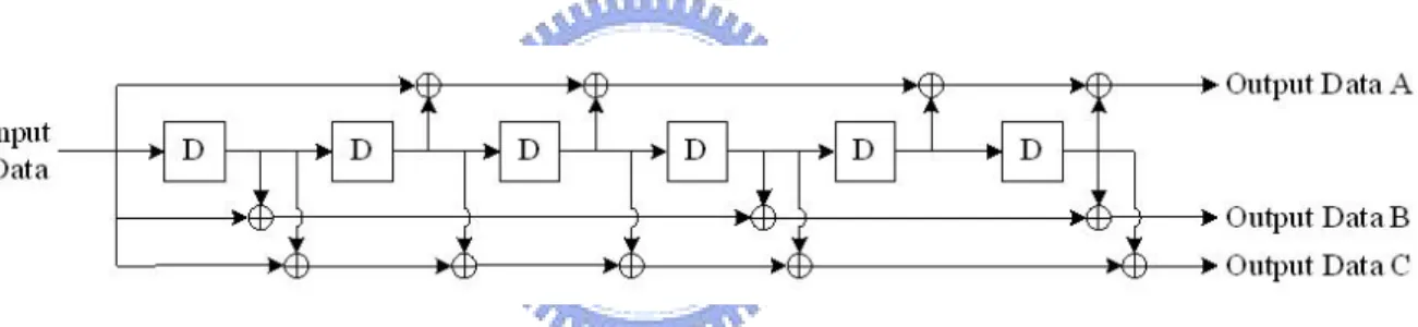
(27) ⎧ ⎛ i T (i ) = S ⎨Floor⎜⎜ ⎝ N T int ⎩. ⎫ ⎞ ⎟⎟ + 10Mod(i, N Tint )⎬ where T(i) = output, S(i) = input, i=0,1,2…, ⎠ ⎭. NCBPS-1 The output of the tone interleaver is then passed through the third stage which cyclic shift the tones of NCBPS bits of bth block. The relationship is as follow, V (b, i ) = T (b, mod(i + A(b), N CBPS )) where V(b,i) = input, T(b,i) = output, i==0,1,2…,. NCBPS-1 A(b) = b*33, b=0,1,2, for conjugate symmetric modes and NCBPS=100. A(b) = b*66, b=0,1,2, for non-conjugate symmetric modes with TSF=2. A(b) = b*33, b=0,1,2,…,5, for non-conjugate symmetric modes with TSF=1.. figure 2.2.4 Convolutional encoder: rate R = 1/3, constraint length K = 7 (source : 802.15.3a proposal). 17.

(28) figure 2.2.5 11/32 coding rate bit-stealing and bit-insertion procedure (source : 802.15.3a proposal). figure 2.2.6 1/2 coding rate bit-stealing and bit-insertion procedure (source : 802.15.3a proposal). 18.

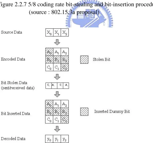
(29) figure 2.2.7 5/8 coding rate bit-stealing and bit-insertion procedure (source : 802.15.3a proposal). figure 2.2.8 3/4 coding rate bit-stealing and bit-insertion procedure (source : 802.15.3a proposal). 19.

(30) The only modulation mapping defined in 802.15.3a is QPSK. The constellation map and bit coding is shown in figure 2.2.9. After mapping, a normalization factor, 1/√2, should be multiply the mapping value to normalize the transmitting power.. figure 2.2.9 QPSK constellation bit encoding (source : 802.15.3a proposal). After interleaving, modulation mapping, and zero-padding prefix adding, a complete packet is formed. The digital signals is then pass through up-sampler, digital filter, DA converter, up-converter, and pass to the antenna. A packet transmitting is complete. The 802.15.3a packet forming procedure is as shown figure 2.2.10. 20.

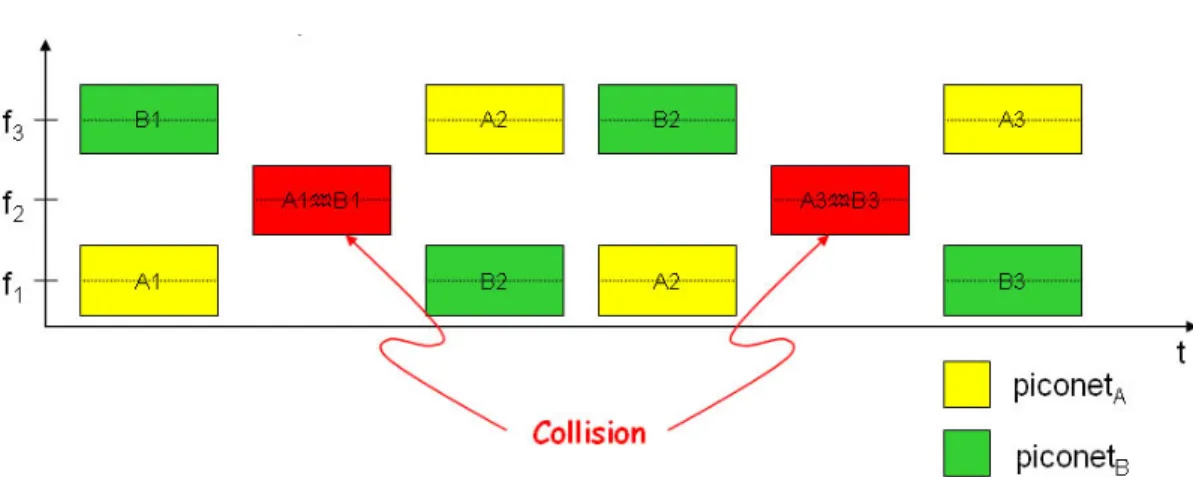
(31) figure 2.2.10. 802.15.3a packet forming procedure. 2.3 Interference of MB-OFDM system MB-OFDM devices can communicate each other and establish a piconet under the control of piconet coordinator (PNC). Since the DEVs in a piconet share the same TFC pattern, PNC can allocate a specific time slot for each connection between DEVs, or employ carrier sense multiple access with collision avoidance (CSMA/CA) to avoid mutual interference. However, MB-OFDM has poor support for simultaneously operating piconets (SOP) due to its slow-hopping pattern, OFDM technology and the limited number of frequency bands available. When geographically overlapped multiple piconets are considered, there is no coordination of transmissions among different piconets, as shown in figure 2.3.1.. 21.

(32) That is, the MB-OFDM must process robustness to interference from other SOPs.. figure 2.3.1 SOP collision situation. 2.4 UWB Channel Model. Over the wireless environment, there are multiple paths between transmitter and receiver to transmit the radio signals. As shown in figure 2.4.1, the left side is an MB-OFDM transmitter and the right side is a receiver. Because of the difference of the distance of each path, the attenuation and the delay differ from path by path. The multipath causes fading effects which are due to interference between two or more versions of the transmitted signal which arrive at the receiver at slight different time.. 22.

(33) figure 2.4.1 Multipath of MB-OFDM. For the purpose of designing a communication system, the propagation channel characteristics must be described to optimize the system. Based on the measurement and study of Intel [2], Saleh-Valenzuela indoor channel model [3] with slight modification is fit for UWB channels. One major characteristic of S-V model is that the rays of multi-path arrive in clusters.. In the S-V model, two Poisson arrival processes are employed to model the arriving of rays. The first Poisson model is for the first path of each path cluster and the second Poisson model is for the paths within each cluster. The mathematical form of the process is as follow: p(Tl | Tl −1 ) = Λ exp[− Λ(Tl − Tl −1 )]. l>0. p(τ k ,l | τ k −1,l ) = λ exp[− λ (τ k ,l − τ k −1,l )]. l>0. Tl = the arrival time of the first path of the l-th cluster; 23.

(34) τk,l = the delay of the k-the path within the l-th cluster relative to the first path arrival time, Tl; Λ = cluster arrival rate; λ = ray arrival rate, i.e., the arrival rate of path within each cluster.. And the overall channel model in mathematical form is:. L. K. hi (t ) = X i ∑∑ α ki ,l δ (t − Tl i − τ ki ,l ) l =0 k =0. where Xi is a shadowing effect gain with log-normal distribution. α ki ,l s are the multipath gain coefficients.. The channel coefficients are defined as follows: α k ,l = p k ,l ξ l β k ,l , 20 log 10(ξ l β k ,l ) ∝ Normal( µ k ,l , σ 12 + σ 22 ) , or ξ l β k ,l = 10. where. n1 ∝ Normal(0, σ 12 ). and. ( µ k , l + n1 + n2 ) / 20. n2 ∝ Normal(0, σ 22 ). are. independent. and. correspond to the fading on each cluster and ray, respectively, 2 −τ / γ E ⎡ ξ l β k ,l ⎤ = Ω 0 e −Tl / Γ e k ,l , ⎢⎣ ⎥⎦. where Tl is the excess delay of bin l and Ω 0 is the mean energy of the first path of the first cluster, and p k ,l is equiprobable +/-1 to account for signal inversion due to reflections. The µk,l is given by µ k ,l =. 10 ln(Ω 0 ) − 10Tl / Γ − 10τ k ,l / γ ln(10). −. (σ 12 + σ 22 ) ln(10) 20. In the above equations, ξ l reflects the fading associated with the lth cluster, and. 24.

(35) β k ,l corresponds to the fading associated with the k ray of the l cluster. th. th. It is notable that the channel model is described in pass band. The model must be converted to equivalent base-band channel to simplify the simulation. The convert procedure derivation is as follows:. [. The passband signal s (t ) = Re sl (t )e j 2πf ct. ]. the signal convoluted with CIR in passband with h(τ ; t) = ∑ α n (t )δ (τ − τ n (t )) n. ⎛⎧ ⎞ ⎫ result in x(t ) = ∑ α n (t ) s[t − τ n (t )] = Re⎜⎜ ⎨∑ α n (t )e − j 2πf cτ n ( t ) sl [t − τ n (t )]⎬e j 2πf ct ⎟⎟ n ⎭ ⎝⎩ n ⎠ and the equivalent low - pass channel c(τ ; t) = ∑ α n (t )e − j 2πf cτ n (t )δ (τ − τ n (t )) n. So. the. overall L. K. hi (t ) = X i ∑∑ e. baseband. channel. of. the. S-V. model. is. − j 2πf c (Tli +τ ki , l ). l =0 k =0. α ki ,l δ (t − Tl i − τ ki ,l ). In the modified S-V channel, there are 6 key parameters that define the model:. Λ = cluster arrival rate; λ = ray arrival rate, i.e., the arrival rate of path within each cluster; Γ = cluster decay factor; γ = ray decay factor; σ 1 = standard deviation of cluster lognormal fading term (dB). σ 2 = standard deviation of ray lognormal fading term (dB). σ x = standard deviation of lognormal shadowing term for total multipath. realization (dB). 25.

(36) These parameters are found by trying to match important characteristics of the channel. Since it’s difficult to match all possible channel characteristics, the main characteristics of the channel that are used to derive the above model parameters were chosen to be the following: • Mean excess delay • RMS delay spread • Number of multipath components (defined as the number of multipath arrivals that are within 10 dB of the peak multipath arrival) • Power decay profile. Since the model parameters are difficult to match to the average power decay profile, the main channel characteristics that are used to determine the model parameters are the first three above. The following table lists some initial model parameters for a couple of different channel characteristics that were found through measurement data.. 26.

(37) Target Channel Characteristics5 Mean excess delay (nsec) ( τ m ). CM 1. CM 2. CM 3. 5.05. 10.38. 14.18. RMS delay (nsec) ( τ rms ). 5.28. 8.03. 14.28. CM 4. 25. 35. NP10dB. 24. 36.1. 61.54. Λ (1/nsec). 0.0233. 0.4. 0.0667. 0.0667. λ (1/nsec). 2.5. 0.5. 2.1. 2.1. Γ. 7.1. 5.5. 14.00. 24.00. γ. 4.3. 6.7. 7.9. 12. σ 1 (dB) σ 2 (dB). 3.3941. 3.3941. 3.3941. 3.3941. 3.3941. 3.3941. 3.3941. 3.3941. σ x (dB). 3. 3. 3. 3. Model Characteristics5 Mean excess delay (nsec) ( τ m ). 5.0. 9.9. 15.9. 30.1. RMS delay (nsec) ( τ rms ). 5. 8. 15. 25. NP10dB. 12.5. 15.3. 24.9. 41.2. NP (85%). 20.8. 33.9. 64.7. 123.3. Channel energy mean (dB). -0.4. -0.5. 0.0. 0.3. Channel energy std (dB). 2.9. 3.1. 3.1. 2.7. NP (85%). Model Parameters. Table 2.4.1 channel model parameters. 27.

(38) Chapter 3 Packet detection and some timing synchronization issues. 3.1 introductions to synchronization tasks Synchronization is an essential task for any digital communication system. Without effective synchronization algorithms, it is not possible to reliably receive the transmitted data. From the perspective of a digital baseband algorithm design engineer, synchronization algorithms pose a major design problem that has to be solved to build a successful product.. OFDM can be used in the context of continuous mode and packet-mode transmission networks. The two transmission schemes require somewhat different approaches to the synchronization problem. Continuous-mode systems transmit data continuously, so a typical receiver can initially spend a relatively long time to acquire the signal and then switch to tracking mode. On the other hand, the synchronization has to be acquired within a very short time after the start of the packet to archive high data rates for packet-mode systems. In MB-OFDM systems, the transmitted signals are OFDM symbols carried by a sequence of carrier frequencies depending on the TFC. Beside the usual OFDM synchronization. tasks. including. packet. detection,. carrier. frequency. synchronization, and timing recovery, the MB-OFDM systems also need a band alignment procedure which aligns the transmitter time-frequency sequence.. 3.2 Packet detection basic issues Basic scheme. 28.

(39) In MB-OFDM systems, there are 30 preambles as training sequences to train the receiver, as mentioned in 2.2. The four patterns for each channel have low cross correlation property to each other. And for each of the preamble, the autocorrelation is close to a delta function. Just like the direct sequence spread spectrum, the preamble can be used to channelize piconet. So the proposed packet detection scheme is a match filter (MF), as shown in figure 3.2.2. For the simplicity of implement, the match filter coefficients are the signs of the preamble, therefore there will be no multiplier in the match filter. The MF is proposed to match the preamble pattern corresponding to the channel which the receiver is going to access. The match filter output is compare to a threshold to determine if the signal comes. For power saving purpose, a constant threshold is preferred in the system. If a proper threshold is setting, the packet detection will be robust to interference and noise.. 29.

(40) figure 3.2.2 MF structure. Interference. When there are two or more piconets operating at the same time, collision will happen in some band. Unfortunately, sometimes the power of interference is stronger than the desired signal. To simplify the detection algorithm, the MF collects the signal of single band. And the packet detection algorithm must be designed robustly to the interference.. First of all, the interference should be modeled in mathematical form to formulate the statistic property of MF output. Take a look at the OFDM symbol,. 30.

(41) s (t ) =. N / 2 −1. N / 2 −1. n=− N / 2. n=− N / 2. ∑ an e j 2πnf0t , which can be represented as s(t ) =. ∑a w n. n. , a weighted sum. of modulated data. If the data are taken as random variables and N is large, s(t) is close to a Gaussian process based on the central limit theorem (CLT).. The OFDM symbol of MB-OFDM systems is composed of 128 tones and each tone carries a QPSK symbol of power equal to unity and tones of indexes {0 64 65 66 67 68} are null tones. The power spectrum density of the MB-OFDM symbol is as shown in figure 3.2.3. And based on Weiner-Khinchin theorem, the autocorrelation of an OFDM symbol is the inverse Fourier transform of the PSD. The autocorrelation is as figure 3.2.4. The autocorrelation function is approximately equal to delta function which means the Gaussian process is uncorrelated.. figure 3.2.3 PSD of MB-OFDM symbol. 31.

(42) figure 3.2.4 Autocorrelation of MB-OFDM symbol. The OFDM symbol of MB-OFDM can be modeled as white Gaussian noise with zero mean because the DC tone is null. It will simplify the analysis of the MF output statistic property while the interference can be modeled as white Gaussian.. Simulation model. There are two kinds of simulation model, the first is to take the SOP interference as white noise and pass through a multipath channel then add to the received signal. In the second model, the received signal is the desired signal incorporated with thermal noise and the signal generated from another piconet. As shown in figure 3.2.5.. 32.

(43) figure 3.2.5 SOP simulation model. Threshold setting. The setting of the threshold is an import part of the detection algorithm. A simple setting method based on AWGN channel is derived. 33.

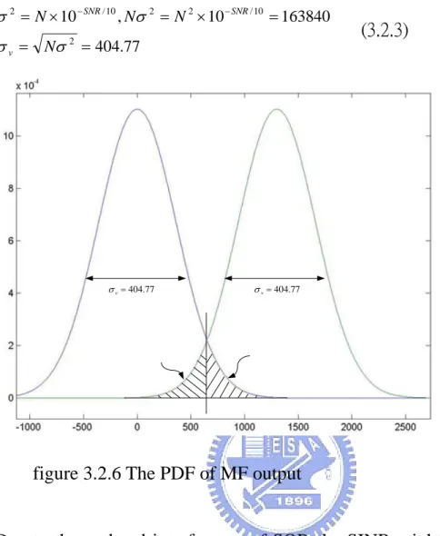
(44) The received signal after sampling is ri = si + ni , where si is the transmitted signal and ni is the noise and interference with distribution, ni ~ N (0,σ 2 ) .. The output of the match filter is mi = i. Let. ∑ pk s k = Ai ,. k =i − N +1. mi = Ai + wi. i. ∑p n. k =i − N +1. k. k. i. ∑ pk sk +. k = i − N +1. i. ∑p n. k =i − N +1. k. k. = wi , so. (3.2.1). The value of Ai depends on the cross-correlation of the symbol and pattern as shown in figure A-1, it is reasonable to assume Ai equal to 0 if the received sequence is not match the pattern desired. And wi is a random variable with distribution N (0, σ v 2 ) , where σ v2 = Nσ 2 . So defined two hypotheses, H0 and H1, where H0 :. mi = wi. H1 :. mi = A + wi. (3.2.2). Based on the proposal of MB-OFDM system, the value of Ai is 1300 when the received signal matches the pattern. So the value of mi is a random variable of Gaussian distribution with variance Nσ2 and bias 0 or 1300 depending on the excess of boundary. The threshold can be set according to the desired false alarm rate or missing rate, as shown in figure 3.2.6. In figure 3.2.6, the SNR is -10 dB for which the noise power is ten times lager than the signal power, and 34.

(45) σ 2 = N × 10 − SNR / 10 , Nσ 2 = N 2 × 10 − SNR / 10 = 163840 σ v = Nσ 2 = 404.77. σ v = 404.77. (3.2.3). σ v = 404.77. figure 3.2.6 The PDF of MF output. Due to the co-band interference of SOP, the SINR might get negative value in dB which means the power of interference is stronger than that of desired signal. The packet detection algorithm in MB-OFDM systems should be robust to this kind of interference. It is important to how much noise the algorithm can tolerate. A plot of the missing rate versus SNR is shown in figure 3.2.7. As shown in this figure, the false alarm rate and missing rate is greatly increasing when SINR lower than -3dB. It is desirable to design another more robust algorithm.. 35.

(46) figure 3.2.7 FAR/Missing rate versus SNR of MF scheme. figure 3.2.8 FAR/Missing rate versus threshold of MF scheme. 3.3 MF with delay correlator. 36.

(47) In an MB-OFDM packet, there are 24 preambles defined in time domain for packet detection. The 24 preambles use the same pattern with a polarity. So there are 8 periodic training symbols in each band. If an auto-correlator with a period of delay is used, the performance will be better. The scheme is as shown in figure 3.3.1. The match filter output is multiplied with a delayed version of its output. Next, the performance of this detection scheme will be analyzed.. figure 3.3.1 delay correlator scheme. The match filter output of the ith sample is as (3.2.3.1), so the delay correlator output is. 37.

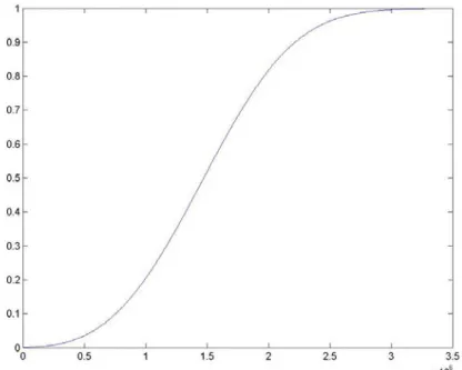
(48) d i = mi mi − N s = ( Ai + wi )( Ai − N s + wi − N s ). (3.3.1). = Ai Ai − N s + Ai wi − N s + Ai − N s wi + wi wi − N s. The two hypotheses are H0 : d i = wi wi − N H1 : d i = A 2 + A( wi − N + wi ) + wi wi − N s. (3.3.2). s. The distribution of hypothesis 0 is the product of two Gaussian variable with mean equal to zero. So the PDF is[4] f (d i ) =. ⎛ di ⎞ ⎟ ⎜ K 0 πσ 2 ⎜⎝ σ 2 ⎟⎠ 1. (3.3.3). where K0(x) is the modified Bessel function of second kind.. But for H1, the PDF of di has no close form. It can be expressed in the form of a double infinite series in Whittaker function. But this form is too complex to use it practically. A simpler one in integration form is derived.. FZ ( z ) = P[ Z < z ] ∞. z/ y. 0. −∞. = ∫ f Y ( y)∫. f X ( x)dxdy + ∫. 0. −∞. f Y ( y)∫. ∞. z/ y. f X ( x)dxdy. 0 ∞ ⎛ ⎛ z / y − A⎞ ⎛ z / y − A ⎞⎞ ⎟⎟dy + ∫ f Y ( y )Q⎜ = ∫ f Y ( y )⎜⎜1 − Q⎜ ⎟dy ⎟ 0 −∞ ⎝ σ ⎠ ⎝ σ ⎠⎠ ⎝. .. (3.3.4). 0 ⎛ − A⎞ ∞ ⎛ z / y − A⎞ ⎛ z / y − A⎞ = Q⎜ ⎟ − ∫0 f Y ( y )Q⎜ ⎟dy + ∫−∞ f Y ( y )Q⎜ ⎟dy ⎝ σ ⎠ ⎝ σ ⎝ σ ⎠ ⎠. where f Y ( y ) =. ⎛ ( y − A )2 ⎞ ⎟ exp⎜⎜ 2 ⎟ 2πσ ⎝ 2σ ⎠ 1. f X ( x) =. ⎛ ( x − A )2 ⎞ ⎟ exp⎜⎜ 2 ⎟ 2πσ ⎝ 2σ ⎠ 1. 38.

(49) Q( x) =. 1 2π. ∫. ∞. x. et. 2. /2. dt. Then the PDF of Z is f Z ( z) =. d 0 d ∞ d ⎛ z / y − A⎞ ⎛ z / y − A⎞ dy + ∫ f Y ( y )Q⎜ P[ Z < z ] = − ∫ f Y ( y )Q⎜ ⎟dy ⎟ dz −∞ dz 0 dz ⎝ σ ⎠ ⎝ σ ⎠. (3.3.5). Although the final term is integration from 0 to infinite, but it is shown that the Q(x) converges to zero very fast. So it is easy to use numerical methods to approximate PDF and CDF. The PDF and CDF is as shown in figure 3.3.2, figure 3.3.3. The CDF plot is more useful for determining the missing rate. When a threshold is set, the corresponding CDF value is the missing rate. Also, the CDF of H0 hypothesis is used to determine the false alarm rate. The corresponding false alarm rate is 1 minus the CDF value of the threshold. The two curves are shown in figure 3.3.4.. figure 3.3.2 PDF of the product of two Gaussian r.v. with bias. 39.

(50) figure 3.3.2 CDF of the product of two Gaussian r.v. with bias. figure 3.3.4 FAR/Missing versus threshold of delay correlator scheme. It is important to check the robustness of the algorithm. First of all, the algorithm should be anti-interference. When threshold is set at the value which has equal false alarm rate and missing rate, the relative variant of the FAR and 40.

(51) missing rate is as shown in figure 3.3.5.. Besides the interference, the carrier frequency offset (CFO) of the algorithm should be considered. The effect of CFO under AWGN channel in baseband is ri = si e j∆fiT + ni. where ri : the ith sample of the received signal s i : the ith sample of the transmitted signal ∆f : carrier frequency offset T : sampling time. (3.3.6). The match filter output is then affected by the CFO. The value of A in (3.2.3.2) is then become N −1. A = ∑ pi si e j 2π∆fiT. (3.3.7). i =0. Theoretically there is some degradation for the value of A. However based on the MB-OFDM proposal, the transmitter and receiver oscillator frequency offset is within ±20 ppm, so the CFO between transmitter and receiver is ±40 ppm in worst case. Assume maximum carrier frequency is 10 GHz, and then the maximum CFO is 400 KHz. The relationship between CFO and the value of A is shown in figure 3.3.6. The maximum degradation happens in ±400 KHz, and the corresponding degradation is -0.1307 dB. The value is small enough to neglect the effect.. 41.

(52) figure 3.3.5 FAR/Missing versus SNR of delay correlator scheme. figure 3.3.6 The cross-correlation degradation due to CFO. 42.

(53) 3.4 The two comparator scheme. Another detector based on two comparators is proposed. The original idea comes from an alternative way of deriving equation (3.3.4).. Let Z=XY, W=X, where X~N(A,σ2). Y~N(A,σ2). The joint PDF function of Z and W is f WZ (w , z ) = f XY ( w ,. z ) J (w, z) w. ∂w ∂x J (w, z) = ∂z ∂x. where. f WZ (w , z ) = =. ∂w ∂y ∂z ∂y. −1. =. 1 w. 1 z f XY ( w , ) w w 1 z f X (w) fY ( ) w w. Then the CDF of Z is FZ ( z ) = ∫. z. ∫. ∞. −∞ −∞. =∫. ∞. −∞. f ZW (u , w)dwdu. z u 1 f X ( w) ∫ f Y ( )dudw − ∞ w w. ∞ 1 z z u u 1 f X ( w) ∫ f Y ( )dudw + ∫ f X ( w) ∫ f Y ( )dudw −∞ − ∞ − ∞ 0 w w w w ∞ z z 0 u u u u = ∫ − f X ( w) ∫ f Y ( )d dw + ∫ f X ( w) ∫ f Y ( )d dw −∞ −∞ − ∞ 0 w w w w 0. =∫ −. 0. = ∫ − f X ( w) ∫ −∞. z/w. ∞. 0. ∞. −∞. z/w. = ∫ f X ( w) ∫. f Y (t )dtdw + ∫. ∞. 0. f Y (t )dtdw + ∫. ∞. 0. (3.4.1). z. f X ( w) ∫ f Y (t )dtdw −∞. f X ( w) ∫. z. −∞. f Y (t )dtdw. 43.

(54) The following steps are as (3.3.4). There is an observation that if the integration interval of w is from some value to ∞ or -∞ to some value instead of being form -∞ to ∞ and the false alarm rate is supposed to decrease greatly with little increasing of miss rate. A change of the integration interval of w means adding a comparator in match filter output. Thus the proposed scheme is as figure 3.4.1.. figure 3.4.1. 2-comparator scheme. The false alarm rate can be calculated, assume th1 and th2 > 0. FAR = P[Z > th1, W > th 2] =∫. ∞. =∫. ∞. =∫. ∞. =∫. ∞. =∫. ∞. ∫. ∞. Th1 Th 2. ∫. ∞. Th 2 Th1. Th 2. Th 2. Th 2. f ZW ( z , w)dwdz f ZW ( z , w)dzdw. ⎧ (w − A)2 ⎫ ⎛ Th1 − Aw ⎞ exp⎨− ⎟dw ⎬Q⎜ 2σ 2 ⎭ ⎝ σw ⎠ w 2π σ ⎩ w. (3.4.2). ⎧ w 2 ⎫ ⎛ Th1 ⎞ Q exp⎨− ⎟dw 2 ⎬ ⎜ w 2π σ ⎩ 2σ ⎭ ⎝ σw ⎠ w. ⎧ w 2 ⎫ ⎛ Th1 ⎞ Q exp⎨− ⎟dw 2 ⎬ ⎜ 2π σ ⎩ 2σ ⎭ ⎝ σw ⎠ 1. 44.

(55) And the missing rate is the match filter output missing or match filter detects but the delay correlator misses. The missing rate is calculated as follow: Missing Rate = P[W < Th2] + P[W > Th2, Z < Th1] ⎛ A - Th2 ⎞ Th1 ∞ = Q⎜ ⎟ + ∫ ∫ f ZW ( z , w)dwdz ⎝ σ ⎠ −∞ Th 2 ⎧ (w − A)2 ⎫⎛ 1 ⎛ A - Th2 ⎞ ∞ ⎛ Th1 − Aw ⎞ ⎞ = Q⎜ + exp ⎟ ∫Th 2 ⎟ ⎟⎟dw ⎨− ⎬⎜⎜1 − Q⎜ 2 w σ 2 σ 2π σ ⎝ σ ⎠ ⎝ ⎠⎠ ⎝ ⎩ ⎭. (3.4.3). The false alarm and missing rate is determined by two parameters, thus a 3-dimension plot is shown in figure 3.4.2 and figure 3.4.3. From these figures, it is found that the missing rate is dominated by the threshold of MF output. If a low missing rate is desired, lower th2 will result in good result. The false alarm rate is also controlled by the threshold of MF, but increasing the delay correlation threshold will get good improvement in false alarm rate.. 45.

(56) figure 3.4.2. figure 3.4.3. FAR versus threshold of two comparator scheme. Miss rate versus threshold of two comparator scheme 46.

(57) For the false alarm rate versus SNR as shown in figure 3.4.5, it has a better false alarm rate with the same missing rate, comparing to the version with only one delay correlation (figure 3.3.5).. figure 3.4.4 FAR/Miss rate versus SNR of two comparator scheme. However, in realistic simulation environment, the oscillator of the receiver is not coherent with the one of the transmitter. Thus there is a phase term resided in the ~. received signal, that is ri = ri e jθ . The phase term will reside in the match filter output and delay correlator output. So the output value before comparator should be taken as absolute one to eliminate the phase term. The modified scheme is as figure 3.4.5.. 47.

(58) figure 3.4.5 The modified version of 2 comparator scheme. The absolute values of the match filter for H0 and H1 then have the distribution of Raileigh and Rician. The relative false alarm rate and missing rate must be recalculated.. For the hypothesis H0, the false alarm probability is:. FAR = ∫. ∞. th 2. =∫. ∞. =∫. ∞. th 2. th 2. ∞ 1 f X ( w) ∫ f Y ( z / w)dzdw th1 w. f X ( w) ∫. ∞. th1 / w. f Y (u )dudw. ⎛ th12 ⎞ ⎟dw ⎜ f X ( w) exp⎜ − 2 2 ⎟ w 2 σ ⎠ ⎝. (3.4.4). ⎛ x2 ⎞ ⎟ x>0 where f X ( x) = 2 exp⎜⎜ − 2 ⎟ σ ⎝ 2σ ⎠ x. f Y ( y) =. ⎛ y2 ⎞ ⎟ y>0 ⎜⎜ − exp 2 ⎟ σ2 ⎝ 2σ ⎠ y. For the hypothesis H1, the missing rate is:. 48.

(59) Missing Rate = ∫. th 2. 0. f X ( w)dw + ∫. ∞. th 2. th1 1 f X ( w) ∫ f Y ( z / w)dzdw 0 w. th1 / w ⎛ A th 2 ⎞ ∞ = 1 − Q1 ⎜ , f Y (u )dudw ⎟ + ∫th 2 f X ( w) ∫0 ⎝σ σ ⎠. ⎛ ⎛ A th 2 ⎞ ∞ ⎛ A th1 ⎞ ⎞ = 1 − Q1 ⎜ , ⎟ + ∫th 2 f X ( w)⎜⎜1 − Q1 ⎜ , ⎟ ⎟⎟dw ⎝σ σ ⎠ ⎝ σ wσ ⎠ ⎠ ⎝. (3.4.5) where Q1 (α , β ) is the Marcum' s Q function ⎛ x 2 + A 2 ⎞ ⎛ Ax ⎞ ⎟⎟ I 0 ⎜ 2 ⎟ f X ( x) = 2 exp⎜⎜ − 2 2 σ σ ⎠ ⎝σ ⎠ ⎝ x. x>0. ⎛ y 2 + A 2 ⎞ ⎛ Ay ⎞ ⎟I 0 ⎜ ⎜⎜ − exp ⎟ y>0 2σ 2 ⎟⎠ ⎝ σ 2 ⎠ σ2 ⎝ I 0 ( x) is modified Bessel function of first kind. f Y ( y) =. y. The second term of (3.4.5) includes integration of Marcum’s Q function, which is hard to be integrated using numerical method. For Marcum’s Q function, when Q(α , β ) α>β, there is a lower bound[4]. 2 ⎡ (α + β )2 ⎤ ⎫⎪ 1 ⎧⎪ ⎡ (α − β ) ⎤ 1 − ⎨exp ⎢− − exp ⎥ ⎢− ⎥ ⎬ ≤ Q1 (α , β ) 2 ⎪⎩ ⎣ 2 ⎦ 2 ⎣ ⎦ ⎪⎭. (3.4.6). Substitute (3.4.6) into (3.4.5) then, ⎛ ⎛ ( Aw + th1)2 ⎞ ⎞ ⎛ ( Aw − th1)2 ⎞ ⎛ A th 2 ⎞ 1 ∞ ⎟ ⎟dw ⎜− ⎟ Missing Rate ≤ 1 − Q1 ⎜ , exp − ⎟ + ∫th 2 f X ( w)⎜⎜ exp⎜⎜ − 2 2 2 2 ⎟⎟ ⎜ ⎟ 2 w w σ 2 σ ⎝σ σ ⎠ 2 ⎠⎠ ⎝ ⎠ ⎝ ⎝. (3.4.7). 49.

(60) figure 3.4.6 FAR versus thresholds of modified two comparator scheme. figure 3.4.6 miss rate versus thresholds of modified two comparator scheme. 50.

(61) From figure 3.4.5 and figure 3.4.6, there is an obvious character that the setting of match filter threshold affects missing rate a lot, but the threshold of delay correlator plays minor part in missing rate. However pulling high the threshold of delay correlator can efficiently decrease the false alarm rate. Assume the threshold of match filter is set as 200, then a false alarm rate/missing rate versus the threshold of delay correlator plot can be obtained as shown in figure 3.4.7.. figure 3.4.7 FAR/Miss rate versus SNR of modified two comparator scheme. 51.

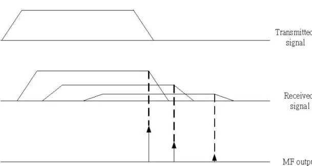
(62) 3.5 The Timing issues. The OFDM symbols can be viewed as the linear combination of orthogonal harmonic waveforms as shown in figure 3.5.1. s ( t ) =. N / 2 −1. ∑ae. n=− N / 2. j 2 π nft. i. , if there is. timing phase offset τT between the transmitter and the receiver, then the received signal becomes N / 2 −1. r (t ) = s (t + τ ) =. ∑ ai e j 2πnf (t +τT ) =. n=− N / 2. N / 2 −1. ∑a e. n=− N / 2. j 2πnfτT. i. e j 2πnft .. (3.5.1). Sampling r(t) with sampling time T, and the symbol time Tu=NT, then r (kT ) =. N / 2 −1. ∑. ai e. j 2π. nτ N. e. j 2π. nk N. (3.5.2). n=− N / 2. without considering the carrier frequency offset. The demodulated data will be multiplied by a phase term, 2π. nτ , and the phase increases linearly with the N. increasing of the carrier tone frequency.. figure 3.5.1 Composite of an OFDM symbol. 52.

(63) The match filter output not only detects the symbol boundary but also provides an acceptable symbol timing point. As shown in figure 3.5.2, the transmitted preamble is delay spread by the channel. But the match filter output only rises as the signal matches the pattern. Thus the match filter output is dependent on the profile of the channel. If a packet boundary is announced by the match filter scheme, it also means the corresponding tap of the channel reaches an acceptable level of power.. figure 3.5.2 The relationship between received signal and MF output. 53.

(64) Chapter 4. Other MB-OFDM synchronization issues. 4.1 Carrier frequency offset (CFO) and timing offset effect in MB-OFDM system. An OFDM symbol is a linear combination of orthogonal harmonic functions with a truncated window function. Assume a rectangular window function is used, then the frequency domain representation of an OFDM symbol is shown is figure 4.1.1. The sampling in frequency domain should be in the peaks of the sinc functions which results in no ICI. But if the transmitter and receiver oscillators mismatch, the sampling in frequency domain will not at the peaks, so the ICI occurs and the desired signal degrades, as shown in figure 4.1.1. ∆f. figure 4.1.1. ICI due to CFO. The effect caused by CFO is the SNR degradation, and the degradation can be 54.

(65) represented as [5]. D≈. E 10 (π∆fT )2 s 3 ln 10 N0. (4.1.1). In MB-OFDM system, the maximum CFO is ±40ppm. For operating in mode 1, the maximum carrier frequency carrier frequency is 4488 MHz, thus the CFO of ±180 KHz is the worst case. The degradation of the SNR versus Es/N0 is then. plotted as figure 4.1.2. And the required Eb/N0 is 4.6 dB when operating in information rate 480 Mb/s, and the equivalent Es/N0 is 7.6 dB. As shown in this figure, the SNR degradation around 7.6 dB is very small compared to Es/N0. So the ICI caused by CFO in MB-OFDM system can be neglected.. figure 4.1.2 SNR degradation versus Es/N0 due to CFO. Besides ICI, the CFO rotates the mth OFDM symbol with angle 2π (m∆fTs + Tg ) , 55.

(66) and each subcarrier of the OFDM symbol suffers this unwanted rotation. So the receiver should compensate this phase shift.. Other issue in timing recovery could include symbol synchronization and sampling clock synchronization. The purpose of symbol synchronization is to find the correct position of the fast Fourier transform window which is introduced in chapter 3.. In [6], the sampling clock offset causes three effects: FFT window drift, ICI, and symbol rotation.. Let ξ =. T ' −T T. where T’ = receiver sampling time T = transmitter sampling time. (4.1.2). The drift at mth OFDM symbol caused by sampling clock offset is:. [. 1 (mN s + N g )T ' − (mN s + N g )T T = (mN s + N g )ξ. FFT window drift =. ] (4.1.3). where N s : sampling points per OFDM symbol N g : guard interval. The FFT window drift effect is as shown in figure 4.1.3.. 56.

(67) figure 4.1.3 The FFT window drift effect due to sampling frequency offset. According to (3.5.2), only FFT window drift effect is considered, the demodulated data will have 2π ~n. a m = a mn e. j 2π. n ( mN s + N g ) N. ξ. n(mN s + N g ) N. ξ phase rotation. Now define. (4.1.4). The demodulated n-th symbol of the m-th OFDM symbol is then ~n. N −1 ~ k. Rmn = a m I n ,n + ∑ a m I k ,n k =0 k ≠n. where I k,n =. 1 sin (π (k (1 + ξ ) − n )) N −1 ⎛ (k (1 + ξ ) − n )⎞⎟ exp⎜ jπ N N ⎛π ⎞ ⎝ ⎠ sin ⎜ (k (1 + ξ ) − n )⎟ ⎝N ⎠. (4.1.5). The SNR degradation due to sampling frequency offset is [6]. 57.

(68) 2 ⎛ E s ⎛ ∆f s ⎞ ⎞⎟ ⎜ ⎜ ⎟ Dn ≈ 10 log10 1 + K n ⎜ N 0 ⎜⎝ f s ⎟⎠ ⎟ ⎝ ⎠ 2 2 N −1 π k 1 where K n = 2 ∑ N k =0 2⎛ π (k − n )⎞⎟ k ≠ n sin ⎜ ⎝N ⎠. (4.1.6). Equation (4.1.6) can be used to evaluate the performance degradation caused by sampling clock offset in an UWB system. As log function is a monotonically increasing function, the maximum SNR degradation happens at the tone of maximum Kn. For MB-OFDM system, the tone index and Kn relationship is shown in figure 4.1.4, and the maximum value of Kn happens at the tone of index 123. Usually the sampling clock is generated from the same oscillator as carrier frequency oscillator. So the sampling clock offset is ±40 ppm. With this Kn, the SNR degradation due to sampling clock offset is shown in figure 4.1.4. The degradation is minor to Es/N0.. figure 4.1.4 The SNR degradation due to sampling frequency offset versus Es/N0. Take a view of equation (4.1.5), the phase rotation of nth tone of mth OFDM symbol can be concluded as:. 58.

(69) θ mn = 2π. n(mN s + N g ) N n(mN s + N g ). ξ + arg[ I n ,n ]. N −1 ξ N N ⎛ mN s + N g N −1 ⎞ = n⎜⎜ 2π ξ +π ξ ⎟⎟ N N ⎝ ⎠ = nκ. = 2π. where κ = 2π. ξ + nπ. mN s + N g N. ξ +π. (4.1.7). N −1 ξ N. The phase rotation is proportional to the tone index, as shown in figure 4.1.5.. figure 4.1.5 Rotation due to SFO and CFO versus tone index. 4.2 The synchronization strategy. From the above discussion, since ICI caused by CFO and sampling clock offset in MB-OFDM play minor role in performance, the synchronization issue becomes how to rotate the phase back and keep tracking the timing phase.. 59.

(70) The synchronization flowchart is as shown in figure 4.2.1. During signal detection, the initial symbol timing is found at the same time as discussed in chapter 3. The channel estimation makes use of the channel estimation portion of the preamble. In every OFDM symbol, 12 pilot tones are inserted. The 12 pilot tones can be used for tracking the phases. As knowing the phase rotation, the receiver should compensate the phase and then demodulate the data. And the phase rotation caused by the timing phase offset should be compensated for the next OFDM symbol.. figure 4.2.1 Synchronization flowchart 60.

(71) Because there is no frequency and phase compensation mechanism, the estimated channel incorporates the same phase rotation due to CFO and sampling clock at the CE symbol, and the rotation will be compensated by the frequency domain equalizer.. Channel estimation. Because MB-OFDM is used in home or office environment and operated in high data rate, it is reasonable to assume the channel impulse response is the same during the whole packet. The most common channel estimation makes use of frequency domain approach.. The received signal in frequency domain is Rmn = H n a mn + Wmn. (4.2.1). and the estimated channel is ^. *. H n = Rmn a mn / a mn. 2. *. = H n + Wmn a mn / a mn. 2. (4.2.2). a mn = 1 for MB-OFDM system, so ^. *. H n = R nm a nm = H n + N nm. where N nm = Wmn a mn. *. (4.2.3). Phase and timing compensation. As shown in figure 4.1.5, the phase rotation due to CFO and sampling clock offset are parallel shift and linear increasing with the tone index. And the pilot position is symmetry about DC tone. So in the tracking loop, the common phase 61.

(72) term is the average of the pilot tone phase rotation. And the slope of the phase line can be used to estimate the sampling phase (e.g. average the slope of each adjacent pilot pair). And then the phase rotation of each subcarrier can be calculated. That is. κ=. 1 Np. ∑ arg( R. n∈pilot tone. n m. ) − arg( p mn ) −θ c. (4.2.4). In equation (4.2.4), the minus of common phase term is necessary. Because the arctan function has an ambiguity of 2πperiod. This phenomenon can be explained by figure 4.2.2. To prevent from the ambiguity, there should not be parallel shift and the slope of the phase increment should not be too large. The parallel shift is canceled by compensating the common phase term. To prevent from phase ambiguity, the receiver should compensate the sampling phase.. Recall equation (4.1.7), the slope of the phase increment is 2π. mN s + N g N. ξ +π. Ng N −1 N −1 ξ . The term 2π ξ +π ξ is compensated by the N N N. FEQ, and the remaining term is 2π. mN s ξ which result from the effect fft N. window drift due to sampling clock offset. According to this slope, the range of phase rotation in an OFDM symbol is 2πmN sξ . It means the sampling phase drift should be controlled to be within one sample. It the sampling clock offset is a constant value, the slope tends to increase or decrease from symbol by symbol depending on the sign of ξ. So when the slope of the phase rotation slope is greater than π/N, it means the fft windows is late for about half a sample and. 62.

(73) the fft window should move forward one sample. When the slope is less than -π /N, it means the fft window is about early for half a sample and the fft window should move backward one sample.. figure 4.2.2 Phase rotation ambiguity due to CFS and sampling frequency offset. Thus the tracking scheme can be shown in figure 4.2.3.. figure 4.2.3 The tracking loop scheme 63.

(74) Chapter 5. Conclusion and future research suggestion. This thesis provides a synchronization strategy and a packet detection method which is robust for simultaneous operating piconets in MB-OFDM systems.. The ICI caused by carrier frequency offset and sampling clock offset is neglected due to its small degradation of SNR. But the synchronization should take care of the phase rotation due to sampling clock offset and carrier frequency offset.. The packet detection algorithm locks one band and correlates the signal with desired preamble pattern to find out whether the channel is occupied. This method provided limited robustness to the interference. An improved algorithm adds a delay auto-correlation mechanism and an additional threshold. The delay correlation result in a better statistic property which decrease the missing and false alarm property. This new scheme has better performance than the match filter algorithm because it uses two symbols to detect the incoming of desired signal.. An alternative scheme might be used for robustness in packet detection of MB-OFDM system. It makes use of the frequency hopping advantage. The usual FHSS system is robust to interference because the jammer can only interfere part of the hopping band. The MB-OFDM system might use another band if the detection band is jammed. This scheme will focus on the detection of interference.. 64.

(75) Reference [1] R.W. Chang, "Synthesis of band-limited orthogonal signals for multichannel data transmission," Bell Systems Technical Journal, vol. 46, pp. 1775-1796, December 1966 [2] J. Foerster and Q. Li, “UWB Channel Modeling Contribution from Intel”, IEEE P802.15-02/279-SG3a. [3] Adel A. M. Saleh and Reinaldo A. Valenzuela “a statistical model for in door multipath propagation” IEEE JSAC, Vol. SAC-5, No.2, pp. 128-137, Feb. 1987. [4] M. K. Simon, Probability Distributions Involving Gaussian Random Variables A Handbook for Engineers and Scientists, Kluwer Academic Publishers, Massachusetts, 2002. [5] Pollet, T., M. van Bladel and M. Moeneclaey, “BER Sensitivity of OFDM Systems to Carrier Frequency Offset and Wiener Phase Noise” IEEE Trans. on Comm. Vol.43 No.2/3/4, pp 191-193, Feb.-Apr. 1995 [6] Thierry Pollet, Paul Spruyt, and Marc Moeneclaey, “The BER Performance using non-synchronized sampling” Proc. of GLOBECOM, pp253-257, 1994 [7] A. Batra et al., “Multiband OFDM physical layer proposal for IEEE 802.15 Task Group 3a”, Multiband OFDM Alliance SIG, Sep. 2004. [8] IEEE Std. 802.15.3, Part 15.3: Wireless Medium Access Control (MAC) and Physical Layer (PHY) Specifications for High Rate Wireless Personal Area Networks (WPANs). LAN/MAN Standards Committee of the IEEE Computer Society, Sep. 2003 [9] Richard van Nee and Ramjee Prasad, OFDM Wireless Multimedia Communications, Artech House, 2000. [10] M. Speth, Stefan A. Fechtel, and H. Meyr, “Optimum receiver design for wireless broad-band systems using OFDM-Part1”, IEEE Trans. Commun., Vol. COM-11, pp.1668-1677, 1999. [11] J. G. Proakis, Digital Communications Fourth Edition, McGraw-Hill, New York, 2000. [12] Schmidl, T. M., and D. C. Cox, “Robust frequency and timing synchronization for OFDM”, IEEE Trans. on Comm., Vol. 45, No. 12, pp.1613-1621, Dec. 1997.. 65.

(76) Appendix MB-OFDM preamble. The MB-OFDM preamble patterns is shown in table A-1 to A-5. And the cross correlation of the pattern with time shift is shown in figure A-1.. figure A-1 the cross-correlation of the preambles with time shift. 66.

(77) Sequence Element. Value. Sequence Element. Value. Sequence Element. Value. Sequence Element. Value. C0. 0.6564. C32. -0.0844. C64. -0.2095. C96. 0.4232. C1. -1.3671. C33. 1.1974. C65. 1.1640. C97. -1.2684. C2. -0.9958. C34. 1.2261. C66. 1.2334. C98. -1.8151. C3. -1.3981. C35. 1.4401. C67. 1.5338. C99. -1.4829. C4. 0.8481. C36. -0.5988. C68. -0.8844. C100. 1.0302. C5. 1.0892. C37. -0.4675. C69. -0.3857. C101. 0.9419. C6. -0.8621. C38. 0.8520. C70. 0.7730. C102. -1.1472. C7. 1.1512. C39. -0.8922. C71. -0.9754. C103. 1.4858. C8. 0.9602. C40. -0.5603. C72. -0.2315. C104. -0.6794. C9. -1.3581. C41. 1.1886. C73. 0.5579. C105. 0.9573. C10. -0.8354. C42. 1.1128. C74. 0.4035. C106. 1.0807. C11. -1.3249. C43. 1.0833. C75. 0.4248. C107. 1.1445. C12. 1.0964. C44. -0.9073. C76. -0.3359. C108. -1.2312. C13. 1.3334. C45. -1.6227. C77. -0.9914. C109. -0.6643. C14. -0.7378. C46. 1.0013. C78. 0.5975. C110. 0.3836. C15. 1.3565. C47. -1.6067. C79. -0.8408. C111. -1.1482. C16. 0.9361. C48. 0.3360. C80. 0.3587. C112. -0.0353. C17. -0.8212. C49. -1.3136. C81. -0.9604. C113. -0.6747. C18. -0.2662. C50. -1.4448. C82. -1.0002. C114. -1.1653. C19. -0.6866. C51. -1.7238. C83. -1.1636. C115. -0.8896. C20. 0.8437. C52. 1.0287. C84. 0.9590. C116. 0.2414. C21. 1.1237. C53. 0.6100. C85. 0.7137. C117. 0.1160. C22. -0.3265. C54. -0.9237. C86. -0.6776. C118. -0.6987. C23. 1.0511. C55. 1.2618. C87. 0.9824. C119. 0.4781. C24. 0.7927. C56. 0.5974. C88. -0.5454. C120. 0.1821. C25. -0.3363. C57. -1.0976. C89. 1.1022. C121. -1.0672. C26. -0.1342. C58. -0.9776. C90. 1.6485. C122. -0.9676. C27. -0.1546. C59. -0.9982. C91. 1.3307. C123. -1.2321. C28. 0.6955. C60. 0.8967. C92. -1.2852. C124. 0.5003. C29. 1.0608. C61. 1.7640. C93. -1.2659. C125. 0.7419. C30. -0.1600. C62. -1.0211. C94. 0.9435. C126. -0.8934. C31. 0.9442. C63. 1.6913. C95. -1.6809. C127. 0.8391. Table A-1 – Time-domain packet synchronization sequence for Preamble Pattern 1 67.

(78) Sequence Element. Value. Sequence Element. Value. Sequence Element. Value. Sequence Element. Value. C0. 0.9679. C32. -1.2905. C64. 1.5280. C96. 0.5193. C1. -1.0186. C33. 1.1040. C65. -0.9193. C97. -0.3439. C2. 0.4883. C34. -1.2408. C66. 1.1246. C98. 0.1428. C3. 0.5432. C35. -0.8062. C67. 1.2622. C99. 0.6251. C4. -1.4702. C36. 1.5425. C68. -1.4406. C100. -1.0468. C5. -1.4507. C37. 1.0955. C69. -1.4929. C101. -0.5798. C6. -1.1752. C38. 1.4284. C70. -1.1508. C102. -0.8237. C7. -0.0730. C39. -0.4593. C71. 0.4126. C103. 0.2667. C8. -1.2445. C40. -1.0408. C72. -1.0462. C104. -0.9563. C9. 0.3143. C41. 1.0542. C73. 0.7232. C105. 0.6016. C10. -1.3951. C42. -0.4446. C74. -1.1574. C106. -0.9964. C11. -0.9694. C43. -0.7929. C75. -0.7102. C107. -0.3541. C12. 0.4563. C44. 1.6733. C76. 0.8502. C108. 0.3965. C13. 0.3073. C45. 1.7568. C77. 0.6260. C109. 0.5201. C14. 0.6408. C46. 1.3273. C78. 0.9530. C110. 0.4733. C15. -0.9798. C47. -0.2465. C79. -0.4971. C111. -0.2362. C16. -1.4116. C48. 1.6850. C80. -0.8633. C112. -0.6892. C17. 0.6038. C49. -0.7091. C81. 0.6910. C113. 0.4787. C18. -1.3860. C50. 1.1396. C82. -0.3639. C114. -0.2605. C19. -1.0888. C51. 1.5114. C83. -0.8874. C115. -0.5887. C20. 1.1036. C52. -1.4343. C84. 1.5311. C116. 0.9411. C21. 0.7067. C53. -1.5005. C85. 1.1546. C117. 0.7364. C22. 1.1667. C54. -1.2572. C86. 1.1935. C118. 0.6714. C23. -1.0225. C55. 0.8274. C87. -0.2930. C119. -0.1746. C24. -1.2471. C56. -1.5140. C88. 1.3285. C120. 1.1776. C25. 0.7788. C57. 1.1421. C89. -0.7231. C121. -0.8803. C26. -1.2716. C58. -1.0135. C90. 1.2832. C122. 1.2542. C27. -0.8745. C59. -1.0657. C91. 0.7878. C123. 0.5111. C28. 1.2175. C60. 1.4073. C92. -0.8095. C124. -0.8209. C29. 0.8419. C61. 1.8196. C93. -0.7463. C125. -0.8975. C30. 1.2881. C62. 1.1679. C94. -0.8973. C126. -0.9091. C31. -0.8210. C63. -0.4131. C95. 0.5560. C127. 0.2562. Table A-2 – Time-domain packet synchronization sequence for Preamble Pattern 2 68.