半古典方法於自旋弛豫和自旋傳輸之應用

物理研究所

碩 士 論 文

半古典方法於自旋弛豫和自旋傳輸之應用

Semiclassical Method Applied to

Spin Relaxation and Spin Transport

研 究 生：蔡政展

指導教授：張正宏 教授

半古典方法於自旋弛豫和自旋傳輸之應用

Semiclassical Method Applied to

Spin Relaxation and Spin Transport

研 究 生：蔡政展 Student： Jengjan Tsai

指導教授：張正宏 Advisors：Cheng-Hung Chang

國 立 交 通 大 學

物 理 研 究 所

碩 士 論 文

A Thesis

Submitted to Institute of Physics College of Science National Chiao Tung University in partial Fulfillment of the Requirements

for the Degree of Master

in

Physics

July 2006

ABSTRACT

Semiclassical Method Applied to

Spin Relaxation and Spin Transport

Tsai, Jengjan

自旋電子學（Spintronics）

在近代物理中是如此活躍的一道學門，

其提供豐富的素材來探究此自然世界和提供推進下一個電子世代之發

展的舞臺。

本 文 主 要 涉 及 在 自 旋 電 子 學 中 極 其 重 要 的

自 旋 弛 豫 （ spin

relaxation，SR）

和

自旋傳輸（spin transport，ST）

之課題。 本文

以

半古典方法（semiclassical method）

來探討

介觀系統（mesoscopic

system）

於

自旋-迴旋交互作用（spin-orbit interaction）

下的電子

自旋行為。 半古典方法之應用乃是此文的關鍵所在。 應用此方法我們

獲得許多有趣的結果,諸如：於各式的自旋-迴旋交互作用下的電子自旋

弛豫和自旋傳輸的

範型（pattern）

,我們分別探討此範型於自旋-迴旋

交 互 作 用 （ 即

有 效 磁 場 ， effective magnetic field

） 之 配 置

（configuration）及其實際大小之作用下的情形；由自旋弛豫和自旋

傳輸之範型得到

規則系統（regular system）

和

混沌系統（chaotic

system）

的本質性差異；有效磁場的

方均根（root-mean-square，RMS）

和其配置之等值性（equivalence）；

自旋弛豫時間（spin relaxation

time，T1）

和

自旋去相時間（spin dephasing time，T2）

於自旋弛豫

例子下之探討；

Rashba 項（Rashba term）

和

Dresselhause 一次項

（Dresselhause linear term）

的等值性；自旋弛豫和自旋傳輸衰竭之

減緩（slow down）

；自旋弛豫和自旋傳輸衰竭之

遏止（stop）

；

自旋波

形編輯器（Spin Waveform Editor，SWE）

等等。

Semiclassical Method Applied to Spin Relaxation and Spin Transport

Tsai, Jengjan

Spintronics the so much active research region in modern physics, o¤ers the matter to explore the fundamental nature of the world and the possible application in next electronic generation.

In this thesis we try to explore some aspects about spintronics, especially focus on spin relaxation (SR) and spin transport (ST) in mesoscopic systems under the spin-orbit coupling e¤ect in terms of modern semiclassicsl approach. The semi-classical approach is the hinge of this thesis. Applying the semisemi-classical method in spin relaxation and spin transport we obtain some interesting results, e.g. spin re-laxation and spin transport patterns under nine (or ten) kinds of di¤erent e¤ective magnetic …eld Bef f which deduced from D’yakonov-Perel’ spin-orbit interaction

mechanism (i.e. the Rashba term and Dresselhause term) treated from two kinds of points of view – normalized and realistic mimic, intrinsic distinguishableness

between regular and chaotic systems from the patterns of SR and ST, the equiva-lence between root-mean-square (RMS) of Bef f and Bef f con…guration, revelation

of spin relaxation time T1 (often called longitudinal or spin-lattice time) and spin

dephasing time T2(also called transverse or decoherence time) in spin relaxation,

equivalence between Rashba term case and Dresselhause linear term case in SR and ST, slow down the spin relaxation and spin transport decay, creating cases of never relaxed and decayable in spin relaxation case and spin transport case, spin waveform editor (SWE), and so on.

I think that I should thank everything! My parents, my relatives, my teachers, my friends, my classmates, my sta¤, living objects, matters, environment et al. they bring so wonderful encounter to me. At this moment I thank especially for my dear parents, my dear instructor (C. H. Chang et al.), my dear friends, my dear sta¤ in NCTU and NTHU (Miss Nora et al.), my dear classmates in NCTU and NTHU, the unique world and so on. Thank you for bringing me so wonderful life! 881

Contents

ABSTRACT iii ABSTRACT v Acknowledgements vii List of Tables xii List of Figures xiii Introduction 1 Part 1. Concepts and Formulism 8 Chapter 1. Spintronics 9 1.1. Foreword 9 1.2. Spin Relaxation and Spin Dephasing 11 1.3. Spin Transport 19 Chapter 2. Operation Environment 21 2.1. Two-dimensional Electron Gas (2DEG) 21 2.2. Proposed Sample Preparation 25

3.2. Spin 1/2 31 3.3. Electron in A Magnetic Field 35 3.4. Time Evolution and Spin Rotation 41 3.5. Spin Precession Extension 45 Chapter 4. Spin-orbit Coupling 48 4.1. Spin-orbit Coupling E¤ect 48 4.2. Spin-orbit Coupling in Solid-state Physics 48 4.3. Spin-orbit Coupling in Quasi-two-dimensional Systems 51 4.4. Inversion-Asymmetry-Induced Spin Splitting 52 4.5. B=0 Spin Splitting and Spin-Orbit Interaction 54 4.6. BIA Spin Splitting in Zinc Blende Semiconductors 56 4.7. SIA Spin Splitting 58 Chapter 5. Spin Dynamics 62 5.1. Preface 63 5.2. Rashba and Dresselhause SOI E¤ect 64 5.3. Spin Evolution 70 Chapter 6. Semiclassical Approach 72 6.1. Chaotic Scattering 72 6.2. Scattering Approach to the Electric Conductance 75

6.3. Semiclassical Transmission Amplitudes 81 6.4. Spin Conductance 85 6.5. Spin Evolution 89 Part 2. Simulation and Discussion 94 Chapter 7. Spin Relaxation 95

7.1. Overview of Spin Relaxation Pattern (Bef f Con…guration Normalized

Case) 97 7.2. Some Aspects of Spin Relaxation Patterns (Bef f Con…guration in

Real Material) 104 7.3. Equivalence between R and D k1Modi…ed Cases 107 7.4. Equivalence between RM S of Bef f and Bef f Con…guration 108

7.5. Relaxation Rate Slow Down Case 110 7.6. Relaxation Rate Never Decay Case 111 Chapter 8. Spin Transport 113

8.1. Overview of the Conductance Decay Patterns (Bef f Con…guration

Normalized Case) 115 8.2. Some Aspects of Conductance Decay Patterns (Bef f Con…guration in

Real Material) 128 8.3. Equivalence between R and D k1Modi…ed Cases 133 8.4. Slow Down Conductance Decay Pattern Case 140 8.5. Never Decay Pattern Case 142

Part 3. Conclusion and Outlook 150 Chapter 10. Conclusion and Outlook 151 References 154

Vita 158

List of Tables

4.1 B=0 spin degeneracy is due to the combined e¤ect of inversion symmetry in space and time. 52

0.1 Typical ballistic cavities. 2 1.1 Qualitative sketch of a Datta-Das spin …eld-e¤ect transistor (SFET). 10 2.1 Conduction and valence band line-up at a junction between an n-type

AlGaAs and intrinsic GaAs. 23 2.2 Schematic layer structure of an inverted In0.53Ga0.47/In0.52Al0.48As

heterostructure and pro…le of the Datta-Das-like SFET. 26 2.3 Schematic layer structure of an inverted In0.53Ga0.47/In0.52Al0.48As

heterostructure and pro…le of the quantum dot for simulation. 27 3.1 n is a unit vector lies in 3D real space. 34 3.2 Magnetic …eld sweeps around on a cone, at angular velocity !. 36 4.1 Qualitative sketch of the band structure of GaAs close to the fundamental

gap. 49

4.2 Qualitative sketch of a wave function, Eq. 4.2, in the envelope function approximation. 55

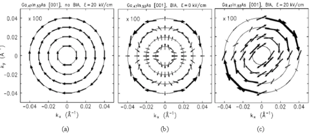
4.3 Lowest-order spin orientation h i of the eigenstates j k_{k i in the}

presence of BIA. 56 4.4 Lowest-order spin orientation h i of the eigenstates j k_{k i in the}

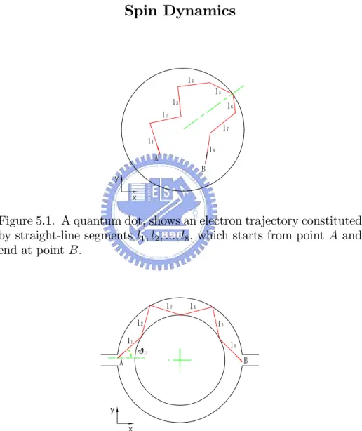
presence of SIA. 59 5.1 A quantum dot, shows an electron trajectory constituted by straight-line

segments: 62 5.2 A quantum ring, shows an electron trajectory constituted by straight-line

segments. 62 6.1 Classicsl distribution of length for stadium (solid line) and rectangular

(dash line) billiards. 74 7.1 Con…guration of Bef f 95

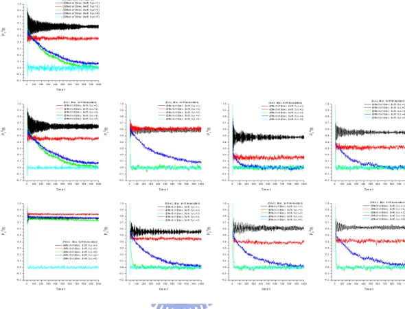
7.2 Five operation systems. 96 7.3 Spin relaxation rate under the viewpoint of e¤ect of direction of Bef f . 99

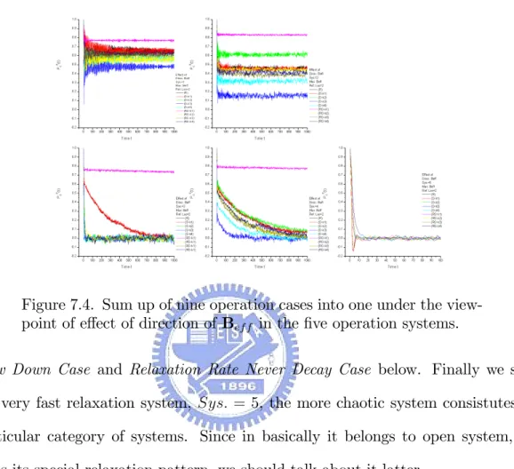
7.4 Sum up of nine operation cases into one under the viewpoint of e¤ect of direction of Bef f. 100

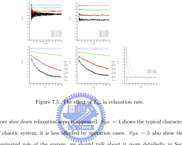
7.5 The e¤ect of Lso. 101

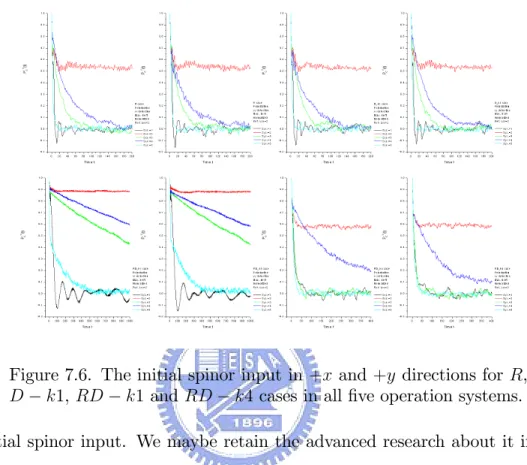
7.6 Cases of the initial spinor input in +x and +y directions for spin relaxation discussion. 102 7.7 The e¤ects of lm (length of mean free path) and size of system. 104

7.9 Sum up of nine operation cases into one under the viewpoint of e¤ect real (calculated) aspect of Bef f. 106

7.10Equivalence between RM S of Bef f and Bef f con…guration in the

relaxation. 108 7.11Relaxation rate slow down case. 110 7.12Relaxation rate never decay case. 111 8.1 Operation systems for spin transport. 113 8.2 hgxxi v.s. 1=Lso under the action of normalized Bef f in more narrow

circular ring system. 116 8.3 hgyyi v.s. 1=Lso under the action of normalized Bef f in more narrow

circular ring system. 117 8.4 hgzzi v.s. 1=Lso under the action of normalized Bef f in more narrow

circular ring system. 118 8.5 hgxxi v.s. 1=Lso under the action of normalized Bef f in less narrow circular

ring system. 121 8.6 hgyyi v.s. 1=Lso under the action of normalized Bef f in less narrow circular

ring system. 122 xv

8.7 hgzzi v.s. 1=Lso under the action of normalized Bef f in less narrow circular

ring system. 123 8.8 hgxxi v.s. 1=Lso under the action of normalized Bef f in more narrow Sinai

billiard system. 124 8.9 hgyyi v.s. 1=Lso under the action of normalized Bef f in more narrow Sinai

billiard system. 125 8.10hgzzi v.s. 1=Lso under the action of normalized Bef f in more narrow Sinai

billiard system. 126 8.11Sum up of hgxxi v.s. 1=Lso under the action of nine kinds of normalized

Bef f in more narrow Sinai billiard system. 127

8.12Sum up of hgyyi v.s. 1=Lso under the action of nine kinds of normalized

Bef f in more narrow Sinai billiard system. 127

8.13Sum up of hgzzi v.s. 1=Lso under the action of nine kinds of normalized

Bef f in more narrow Sinai billiard system. 128

8.14hgxxi v.s. 1=Lso under the action of normalized Bef f in less narrow Sinai

billiard system. 129 8.15hgyyi v.s. 1=Lso under the action of normalized Bef f in less narrow Sinai

billiard system. 130 8.16hgzzi v.s. 1=Lso under the action of normalized Bef f in less narrow Sinai

billiard system. 131 xvi

8.18Sum up of hgyyi v.s. 1=Lso under the action of nine kinds of normalized

Bef f in less narrow Sinai billiard system. 132

8.19Sum up of hgzzi v.s. 1=Lso under the action of nine kinds of normalized

Bef f in less narrow Sinai billiard system. 133

8.20Comparison between the normalized Bef f con…guration and Bef f

con…guration in real material for D k2case in circular ring system. 134 8.21Comparison between the normalized Bef f con…guration and Bef f

con…guration in real material for RD k4 case in circular ring system. 135 8.22Comparison between the normalized Bef f con…guration and Bef f

con…guration in real material for D k1case in Sinai billiard. 136 8.23Comparison between the normalized Bef f con…guration and Bef f

con…guration in real material for RD k4 case in Sinai billiard. 137 8.24Equivalence between R and D k1modi…ed cases. 138 8.25Example of equivalence between R and D k1 modi…ed cases in circular

ring system. 139 8.26Example of equivalence between R and D k1 modi…ed cases in Sinai

billiard system. 140 xvii

8.27Example of slow down conductance decay pattern case in RD k1and RD k4 cases. 141 8.28Examples of never decay spin conductance pattern case. 144 9.1 Square waveform patterns. 146 9.2 Design of Spin Waveform Editor (SWE) device 1. 147 9.3 Design of Spin Waveform Editor (SWE) device 2. 147

It is so excited to touch and explore the natural world. Spintronics the so much active research region in modern physics, o¤ers the matter to explore the fundamental nature of the world and the possible application in next electronic generation. In this thesis we try to explore some aspects about spintronics, espe-cially focus on spin relaxation (SR) and spin transport (ST) in mesoscopic systems, see Fig. 0.1, under the spin-orbit coupling e¤ect in terms of modern semiclassicsl approach. Due to the ‡ush development in theoretical and experimental research in spintronics, we strongly expect oncoming of experimental breakthrough to ver-ify the so much theoretical prediction and advance the spintronics research. We also hope that our research in the thesis could nudge spintronics towards a more fulgent future.

The semiclassical approach is the hinge of our thesis. Applying the semiclassical method in spin relaxation and spin transport we obtain some interesting results, e.g. spin relaxation and spin transport patterns under nine (or ten) kinds of di¤er-ent e¤ective magnetic …eld Bef f which deduced from D’yakonov-Perel’spin-orbit

interaction mechanism (i.e. the Rashba term and Dresselhause term) treated from

2

Figure 0.1. (a) Typical ballistic cavity coupled to reservoirs char-acterized by chemical potential 1 and 2 for mesoscopic structure. (b) Typical ballistic cavity for closed mesoscopic structure.

two kinds of points of view –normalized and realistic mimic, intrinsic distinguish-ableness between regular and chaotic systems from the patterns of SR and ST, the equivalence between root-mean-square (RMS) of Bef f and Bef f con…guration,

revelation of spin relaxation time T1 (often called longitudinal or spin-lattice time)

and spin dephasing time T2(also called transverse or decoherence time) in spin

re-laxation, equivalence between Rashba term case and Dresselhause linear term case in SR and ST, slow down the spin relaxation and spin transport decay, creating cases of never relaxed and decayable in spin relaxation case and spin transport case, spin waveform editor (SWE), and so on. Since the signi…cant role of semi-classical method in this thesis, here we shortly talk about something relevant to it and then we give an rough outline of this thesis to be as an introduction.

The mesoscopic regime is attained in small condensed matter systems at su¢ -ciently low temperature for the electrons to propagate coherently across the sample [1]. The phase coherence of the electron wave-function is broken by an inelastic

event (coupling to an external environment, electron-phonon or electron-electron scattering, etc.) over a distance L larger than the size of the system a. In a more precise language, we should not talk of electrons, which are strongly interacting, but of Landau quasiparticles, which are the weakly interacting carriers (at low energies and small temperature) moving in a self consistent …eld. The quasiparti-cle lifetime gives the limitation on L arising from electron-electron interactions. Following the standard practice, we will refer to the carriers as electrons and we will not distinguish between the electrostatically imposed external potential and the self consistent …eld.

The view of a mesoscopic system as a single phase-coherent unit allow us to deal with a one-particle problem, where the theoretical concepts of Quantum Chaos are more simply applied. However, this simplistic approach does not describe the physical reality completely since in real life L is larger than a but never strictly in…nite. The fact that Mesoscopic Physics is not such an ideal laboratory for Quantum Chaos makes the richness of their relationship. Mesoscopic system are extremely useful to study the interplay between quantum and classical mechanics. Mesoscopic Physics was initially focused on disordered metals, where the clas-sical motion of electrons is a random walk between the impurities. The phase-coherence in the multiple scattering of electrons gives rise to corrections to the classical (Drude) conductance. The small parameter is kFl , with kF = 2 = F the

4 Fermi wave-vector and l the elastic mean-free-path (i.e. the typical distance trav-eled by the electron between successive collision with the impurities). Mesoscopic disordered conductors are then characterized by F l a L .

It is in a second generation of mesoscopic systems, semiconductor microstruc-tures, that the connection with Quantum Chas has been more successfully devel-oped. Extremely pure semiconductor (GaAs/AlGaAs) heterostructures make it possible to create a two-dimensional electron gas (2DEG) by quantizing the mo-tion perpendicular to the interphase. Given the crystalline perfecmo-tion and the fact that the dopants are away from the plane of the carriers, an electron can travel a long distance before its initial momentum is randomized. This typical distance, the transport mean-free-path lT, is generally larger than the elastic mean-free-path

(due to small-angle scattering [2]) and it can achieve values of 5 15 m.

Various techniques have been developed to produce a lateral con…nement in the 2DEG and de…ne one-dimensional (quantum wire) and zero-dimensional (quantum boxes or cavities) structure. Spatial resolutions of the order of a micro allow to de…ne, at the level of the 2DEG, mesoscopic structures smaller than the elastic mean-free-path, paving the way to the ballistic regime [3][4][5]. When a lT the

classical motion of the two-dimensional electrons is given by the collisions with the walls de…ning the cavity, with a very small drift due to the weak impurity potential. In usual ballistic transport the disorder e¤ects are very small, and the distinction between ballistic and clean regimes is often skipped.

It is important to realize that the constraints arising from the measurement limit the type of problems to study. We do not try to deal with microscopic systems where the level spacing can become larger than the temperature broadening kBT.

The fruitful connection between Quantum Chaos and Mesoscopic Physics has to be established from the observables that are accessible in the laboratory. The physical property of ballistic microstructures which is most easily measured is their electrical resistance, and as a consequence, an important wealth of experimental results on ballistic transport has been obtained in the last decade [6][7][8][9][10][11][12]. In order to measure the electrical resistance we have to open the cavities, connecting them to measuring devices that are necessarity macroscopic and can be thought as electron reservoirs Fig. 0.1 (a).

Semiclassical approaches were essential at the advent of Quantum Mechanics and have ever since remained a privileged tool for developing our intuition on new problems and for performing analytical calculations as well [13]. The semiclas-sical approximation in one-dimensional is referred in standard textbooks as the WKB (Wentzel-Kramers-Brillouin) method and allows to obtain closed expres-sions for eigenenergies and eigenfunctions. The extension to higher dimenexpres-sions is built from the Van Vleck approximation to the propagator, expressed as a sum over classical trajectories, each of them associated with a weight given by a sta-bility prefactor and a phase depending on the classical action. The consistent use of the stationary-phase method whenever an integral has to be evaluated allows us to link classical mechanics with other quantum protagonists, like the Green

6 function, the density of states, matrix elements, scattering amplitudes, etc. the dependence of the properties of a quantum system on the underlying clasical me-chanics can then be established, and this is why the semiclassical approach is so widely used in the studies of Quantum Chaos. For the usual densities of the 2DEG ( 1012_cm 2_{) [1] the Fermi wave-length are of the order of 40nm. The}

semiclassi-cal approximation is therefore justi…ed in the study of mesoscopic ballistic cavities since F a lT l :

We note that the …rst generation of mesoscopic systems, the disordered metals, have mainly been analyzed within diagrammatic perturbation theory. Since the scattering centers of disorder metals (defects, impurities, interstitials, etc.) are of atomic dimensions the single scattering events have to be treated quantum mechanically. Therefore the semiclassical description of disordered system is mixed one, built from a classical propagation between quantum scatterings. Assuming that the classical single scattering events have a random outcome and invoking an ensemble average, we are lead to a di¤usive motion of electrons. The situation is then quite di¤erent from that of ballistic systems, were the classical trajectories are completely determined by the geometry and the dynamics can be chaotic or integrable depending on the shape of the cavity. Also, the notion of impurity average, so crucial in disordered systems, is usually replaced in the ballistic regime by averages over energy or over samples.

This thesis is organized as follows. It is divided by three parts. First part, Concepts and Formulism, we talk about the minimal necessary relevant concepts

and formulism to this thesis and deduce some expressions for understanding the thesis. It includes Spintronics, Operation Environment, Spin, Spin-orbit Coupling, Spin Dynamics, and Semiclassical Approach of spin transport and spin relaxation, and so on. Second part, Simulation and Discussion, we present our simulation re-sults and deduce some expressions relevant to the corresponsive topics. It is mainly divided by three portions. First portion we discuss the Spin Relaxation. Here we explore both the regular and chaotic systems and di¤erent collision (scattering) situation under the e¤ect of Rashba and Dresselhause terms. We …nd some very interesting and surprising results about the spin relaxation decay rate. We get an expression which depicts satisfactory aspects for these spin relaxation rate and so on. Second portion we focus on the Spin Transport, the regular systems and chaotic systems under Rashba and Dresselhause (linear and/or cubic) terms e¤ect are discussed. We also examine the equivalence between Rashba and Dresselhause linear terms in spin transport and relaxation under some point of view and men-tion a special case of the arrangement of Rashba and Dresselhause linear terms to produce the never decay spin transport current and so forth. Final portion we pro-pose and design a spintronic device –Spin Waveform Editor (SWE). This device can be applied as a switch or/and as a resource for research and instruction usage. Part 3, Conclusion and Outlook, we give a conclusion that talks about some defect and leakage in our research, and the outlook which indicates something interesting and hopeful respect in further research. Reference is lay in the …nal.

Part 1

Spintronics

1.1. Foreword

Spintronics is a multidisciplinary …eld whose central theme is the active ma-nipulation of spin degrees of freedom in solid-state systems. Here the term spin stands for either the spin of a single electron or the average spin of an ensemble of electrons, manifested by magnetization. The control of spin is then a control of either the population and the phase of the spin of an ensemble of particles, or a coherent spin manipulation of a single or a few-spin system. The goal of spintron-ics is to understand the interaction between the particle spin and its solid-state environments and to make useful devices using the acquired knowledge. Funda-mental studies of spintronics include investigations of spin transport in electronic materials, as well as of spin dynamics and spin relaxation. Typical questions that are posed are (a) what is an e¤ective way to polarize a spin system? (b) how long is the system able to remember its spin orientation? and (c) how can spin be detected?

Now let us illustrate the generic spintronic scheme on a prototypical device, the Datta-Das spin …eld-e¤ect transistor (SFET, [14]), depicted in Fig. 1.1. The scheme shows the structure of the usual FET, with a drain, a source, a narrow

10

Figure 1.1. Qualitative sketch of a Datta-Das spin …eld-e¤ect tran-sistor (SFET) [14]. Larger black arrows indicate the spin polar-ization in the ferromagnetic contact (FM) and the semiconducting channel. Smaller black arrows indicate the e¤ective magnetic …eld Bef f(kx) in the semiconducting channel. A top gate is used to tune

the spin precession by appluing an electric " perpendicular to the Qualitative sketch of a Datta-Das spin …eld-e¤ect transistor (SFET).

channel, and a gate for controlling the current. The gate either allows the current to ‡ow (ON) or does not (OFF). The spin transistor is similar in that the result is also a control of the charge current. The di¤erence, however, is in the physical realization of the currenr control. In the Datta-Das SFET the source and the drain are ferromagnets acting as the injection and detection of the electron spin. The drain injects electrons with spins perpendicular to the transport direction. The electrons are transported ballistical through the channel. When they arrive at the drain, their spin is detected. In simpli…ed picture, the electron can enter the drain (ON) if its spin points in the same direction as the spin of the drain. Otherwise it is scattered away (OFF). The role of the gate is to generate an e¤ective magnetic …eld as Figure 1.1 shown, arising from the spin-orbit coupling in the substrate material,

from the con…nement geometry of the transport channel, and the electrostatic potential of the gate. This e¤ective magnetic …eld causes the electrons spins to precess. By modifying the voltage, one can cause the precession to lead to either parallel or antiparallel (or anything between) electron spin at the drain, e¤ectively controlling the current.

Well! Even though the name Spintronics is rather novel (the term was coined by Wolf, S. A. in 1996, as a name for a DARPA initiative for novel magnetic ma-terials and devices), contemporary research in spintronics relies closely on a long tradition of results obtained in diverse areas of physics (e.g., magnetism, semicon-ductor physics, superconductivity, optics, and mesoscopic physics) and establishes new connections between its di¤erent sub…elds. Spintronics also bene…ts from a large class of emerging materials, such as ferromagnetic semiconductors [15][16], organic semiconductors [17], organic ferromagnets [18], high-temperature super-conductors, and carbon nanotubes [19][20], which can bring novel functionalities to the traditional devices. In one word, there is a continuing need for fundamental studies before the potential of spintronic applications can be fully realized [21]. This is right part of the goal of this thesis.

1.2. Spin Relaxation and Spin Dephasing

Spin relaxation and spin dephasing are process that lead to spin equilibra-tion and are thus of great important for spintronics. The fact that nonequilib-rium electronic spin in metals and semiconductors lives relatively long (typically

12 a nanosecond), allowing for spin-encoded information to travel macroscopic dis-tances, is what makes spintronics a viable option for technology. After introducing the concepts of spin relaxation and spin dephasing time respectively, which are commonly called s, we just brie‡y talk about the major physical mechanisms

re-sponsible for spin equilibration in nonmagnetic electronic systems: Elliott-Yafet, D’yakonov-Perel’, Bir-Aronov-Pikus, and hyper…ne interaction processes [21]. 1.2.1. Spin Relaxation Time and Spin Dephasing Time

Spin relaxation and spin dephasing of a spin ensemble are traditionally de…ned within the framework of the Block-Torry equations [22][23] for magnetization dy-namics. For mobile electrons, spin relaxation time T1 (often called longitudinal or

spin-lattice time) and spin dephasing time T2(also called transverse or

decoher-ence time) are de…ned via the equation for the spin precession, decay, and di¤usion of electronic magnetization M in an applied magnatic …eld B(t) = B0z + B^ 1(t),

with a static longitudinal components B0 (conventionally in the z direction), and

frequently, a transverse oscillating part B1 perpendicular to z [23][24]:

(1.1) @Mx @t = (M B)x Mx T2 + D_r2Mx, (1.2) @My @t = (M B)y My T2 + D_r2My,

(1.3) @Mz

@t = (M B)z

Mz Mz0

T1

+ D_r2Mz,

Here = _{Bg=~ is the electron gyromagnetic ratio ( B} is the Bohr magneton and g is the electronic g factor), D is the di¤usion coe¢ cient (for simplicity we assume an isotropic or a cubic solid with scalar D), and M0

z = B0 is the thermal

equilibrium magnetization with denoting the system’s static susceptibility. The Bloch equations are phenomenological, describing quantitatively very well the dy-namics of mobile electron spins (more properly, magnetization) in experiments such as conduction-electron spin resonance and optical orientation. Although relaxation and decoherence processes in a many-spin system are generally too complex to be fully described by only two parameters, T1 and T2 are nevertheless an extremely

robust and convenient measure for quantifying such processes in many cases of in-terest. To obtain microscopic expressions for spin relaxation and dephasing times, one starts with a microscopic description of the spin system (typically using the density-matrix approach), desires the magnetization dynamics, and compares it with the Bloch equations to extract T1 and T2:

Time T1 is the time it takes for the longitudinal magnetization to reach

equi-librium. Equivalently, it is the time of thermal equilibration of the spin population with the lattice. In T1 processes an energy has to be taken from the spin system,

14 an ensemble of transverse electron spins, initially precessing in phase about the longitudinal …eld, to lose their phase due to spatial and temporal ‡uctuations of the precessing frequencies. For an ensemble of mobile electrons the measured T1

and T2 come about by averaging spin over the thermal distribution of electron

momenta. Motional (dynamical) narrowing is an inhibition of phase change by random ‡uctuations. Consider a spin rotating with frequency !0. The spin phase

changes by = !0t over time t. If the spin is subject to a random force that

makes spin precession equally likely clockwise and anticlockwise, the average spin phase does not change , but the root-mean-square phase change increases with time as (< 2 _>) 1=2 _(!

0 c)(t= c)1=2, where c is the correlation time of the

random force, or the average time of spin precession in one direction. This is valid for rapid ‡uctuations, !0 c 1. The phase relaxation time t is de…ned as the

time over which the phase ‡uctuations reach unity: 1=t = !2 0 c.

In isotyopic and cubic solids T1 = T2 if B0 1= c, where c is the

so-called correlation or interaction time: 1= c is the rate of change of the e¤ective

dephasing magnetic …eld. Phase losses occur during time intervals of c. If the

system is anisotropic, the equality T1 = T2 no longer holds, even in the case of full

motional narrowing of the spin-spin interactions and g-factor broadening. Using simple qualitative analysis Yafey in 1963 showed that, while there is no general relation between the two times, the inequality T2 6 2T1 holds, and that T2 changes

with the direction by at most a factor of 2. The equality of the two times is very convenient for comparing experiment and theory, since measurements usually

yield T2 , while theoretically it is often more convenient to calculate T1. In many

cases a single symbol c is used for spin relaxation and dephasing (and called

indiscriminately either of these terms), if it does not matter what experimental situation is involved, or if one is working at small magnetic …elds.

In our simulation I think that we mainly calculate (simulate) spin relaxation time T1 (or called longitudinal or spin-lattice time), in Chapter 7 we also simulate

few illustrative cases which show the aspects of spin dephasing time T2 (or called

transverse or decoherence time), we …nd a reasonable explanation to reach the consistency about the statement T2 6 2T1.

Experiments detecting spin relaxation and decoherence of conduction electrons can be grouped into two broad categories: (a) those measuring spectral charac-teristics of magnetization depolarization and (b) those measuring time or space correlations of magnetization [21]. Well! Here we do not attempt to discuss the aspects of experiments, so we stop discussing further more.

1.2.2. Mechanism of Spin Relaxation

Four mechanisms for spin relaxation of conduction electrons have been found rel-evant for metals and semiconductors: the Elliott-Yafet, D’yakonov-Perel’, Bir-Aronov-Pikus, and hyper…ne-interaction mechanisms. (Here we do not consider magnetic scattering, that is, scattering due to an exchange interaction between conduction electrons and magnetic impurities.) In the Elliott-Yafet mechanism electron spins relax because the electron wave functions normally associated with

16 a given spin have an admixture of the opposite-spin states, due to spin-orbit cou-pling induced by ions. The D’yakonov-Perel’mechanism explains spin dephasing in solids without a center of symmetry. Spin dephasing occurs because electrons feel an e¤ective magnetic …eld, resulting from the lack of inversion symmetry and from the spin-orbit interaction, which changes in random directions every time the elec-tron scatters to a di¤erent momentum state. The Bir-Aronov-Pikus mechanism is important for p-doped semiconductors, in which the electron-hole exchange inter-action gives rise to ‡uctuating local magnetic …elds ‡ipping electron spins. Finally, in semiconductor heterostructures (quantum wells and quantum dots and so on) based on semiconductors with a nuclear magnetic moment, it is the hyper…ne inter-action of the electron spins and nuclear moments which dominates spin dephasing of localized or con…ned electron spins [21]. In this thesis, we mainly consider the spin relaxation in two-demensional III-V semiconductor heterostructures due to D’yakonov-Perel’mechanism, so we just exhibit the D’yakonov-Perel’Mechanism a little more, and ignore to talk about other mechanisms more detailedly.

An e¢ cient mechanism of spin relaxation due to spin-orbit coupling in systems lacking inversion symmetry was found by D’yakonov and Perel’in 1971. Without inversion symmetry the momentum states of the spin-up and spin-down electrons are not degenerate: Ek+ 6= Ek . Kramer’s theorem still dictates that Ek+ =

E k . Most prominent examples of materials without inversion symmetry come

from groups III-V (such as GaAs) and II-VI (ZnSe, etc.) semiconductor, where inversion symmetry is broken by the presence of two distinct atoms in the Bravais

lattice. Elemental semiconductors like Si possess inversion symmetry in the bulk, so the D’yakonov-Perel’mechanism does not apply to them. In heterostructures the symmetry is broken by the presence of asymmetric con…ning potentials.

Spin splittings induced by inversion asymmetry can be described by introducing an intrinsic k-dependent magnetic …eld Bi(k) around which electron spins precess

with larmor frequency (k) =e=m Bi(k). The intrinsic …eld derives from the

spin-orbit coupling in the band structure. The corresponding Hamiltonian term describing the precession of electrons in the conduction band is

(1.4) H(k) = 1

2~ (k)

where are the Pauli matrices. Momentum-depedent spin precession described by H, together with momentum scattering characterized by momentum relaxation time p, leads to spin dephasing. While the microscopic expression for (k)needs

to be obtained from the band structure, treating the e¤ects of inversion asymmetry by introducing intrinsic precession helps to give a qualitative understanding of spin dephasing. It is important to note, however, that the analogy with real Larmor precession is not complete. An applied magnetic …eld induces a macroscopic spin polarization and magnetization, while H of Eq. (1.4) produces an equal number of spin-up and spin-down states.

18 Two limiting cases can be considered: (a) p av > 1 and (b) p av 6 1,

where av is an average magnitude of the intrinsic larmor frequency (k) over

the actual momentum distribution. Case (a) corresponds to the situation in which individual electron spins process a full cycle before being scattered to another mementum state. The total spin in this regime initially dephases reversibly due to the anisotropy in (k). The spin dephasing rate, which depends on the distribution of values of (k), is in general proportional to the of the distribution: 1= s

. The spin is irreversibly lost after time p, when randomizing scattering takes

place.

Case (b) is what is usually meant by the D’yakonov-Perel’ mechanism. This regime can be viewed from the point of view of individual electrons as a spin pre-cession about ‡uctuating magnetic …elds, whose magnitude and direction change randomly with the average time step of p. The electron rotates about the intrinsic

…eld at an angle = av p, before experiencing another …eld and starting to

ro-tate with a di¤erent speed and in a di¤erent direction. As a result, the spin phase follows a random walk: after time t, which amounts to t= p steps of the random

walk, the phase progresses by (t) pt= p. De…ning s at the time at which

(t) = 1, the usual motional narrowing result is obtained: 1= s 2av p.

The faster the momentum relaxation, the slower the spin dephasing. The di¤erence between cases (a) and (b) is that in case (a) the electron spins form an ensemble that directly samples the distribution of (k), while in case (b) it is the distribution of the sums of the intrinsic Larmor frequencies (the total phase

of a spin after many steps consists of a sum of randomly selected frequencies multiplied by p), which, according to the central-limit theorem, has a signi…cantly

reduced variance. Both limits (a) and (b) and the transition between them have been experimentally demonstrated in n-GaAs/AlGaAs quantum wells by observing temporal spin oscillations over a large range of temperatures (and thus p) [26].

1.3. Spin Transport

Maybe Transport will be not a simple topic for master graduate student. Under di¤erent operation environment, the various transport aspects could be exhibited. For example, comparing mean free path l with characteristic dimensions of the system a, one can discriminate between di¤usive, l a, quasi-ballistic, l > a, and ballistic, l a, transport. Such a classi…cation appears incomplete in the situation where di¤erent dimensions of the sample are substantially di¤erent. If phase coherence is taken into account, the scales L and LT become important,

and the situation appears more rich and interesting. In our thesis we assume the electron exhibits the ballistic transport, so here we don’t intend to show the content of di¤usive transport, we just indicate the key point of ballistic transport, that is a very powerful method in physics of small systems the so-called Landauer approach.

The main principle of this approach is the assumption that the system in ques-tion is coupled to large reservoirs where all inelastic processes take place. Con-sequently, the transport through the systems can be formulated as a quantum

20 mechanical scattering problem. Thus one can reduce the non-equilibrium trans-port problem to a quantum mechanical one. Another imtrans-portant assumption is that the system is connected to reservoirs by ideal quantum wires which behave as waveguides for the electron waves. And we also give an very important assump-tion for the transport topics, we assume that the charge transport is independent (un-coupled) to spin transport which it is attached to the wave functions of charge particle. This assumption o¤ers the base to consider the spin evolution indepen-dently to the charge (electron) traveling. Our simulations are all established under this such assumption. We should discuss this more detailedly in Chapter 6.

Operation Environment

2.1. Two-dimensional Electron Gas (2DEG)

By dynamically two-dimensional we mean that the electrons or holes have quan-tized energy levels for one spatial dimension, but are free to move in two spatial dimensions. Thus the wave vector is a good quantum number for two dimensions, but not for the third. These systems are not two-dimensional in a strict sense, both because wave functions have a …nite spatial extent in the third dimension and because electromagnetic …elds are not con…ned to a plane but spill out into the third dimension. Theoretical predictions for idealized two-dimensional systems must therefore be modi…ed before they can be compared with experiment.

Here we shall generally con…ne our discussion to systems for which parameters can be varied in a given sample, usually by application of an electrical stress. Sys-tems of this sort generally occur in what may broadly be called heterostructures. The best known example are carriers con…ned to the vicinity of junctions between insulators and semiconductors, between layers of di¤erent semiconductors, and between vacuum and liquid helium. For most of these systems the carrier concen-tration can be varied, so that a wealth of information can be obtained from one

22 sample. They all have at least one well-de…ned interface which is usually sharp to a nanometer or less.

The e¤ects of changes in surface conditions on the conductance of a semicon-ductor sample have been studied for many years. Such measurements are usually called …eld-e¤ect measurements because a major physical variables is the electric …eld normal to the semiconductor surface. One important way to change the sur-face condition, and therefore the sursur-face electric …eld, is through the control of gaseous ambients, see for example: Brattain, W. H.-Bardeen, J. cycle experiment in 1953, and Mary, A. experiment in 1974. A disadvantage of the early mea-surements was that the conductance of the entire sample was measured, and the surface e¤ects were extracted by taking di¤erences or derivatives as the ambient was changed. In conjuction with …eld-e¤ect measurements, theories for the depen-dence of the mobility of carriers near the surface on the surface conditions were developed and re…ned. Most of the early work was based on the phenomenological notion of di¤use and specular re‡ection at the surface, as …rst used by Fuchs, K. in 1938 in studing transport in metal …lms. .

Investigation of space-charge layers on narrow-gap III-V semiconductors also started in the mid-1960s. However, the di¢ culty of obtaining samples with good quality has long prevented progress in this system. After many people e¤ort and many years later, the development on heterostructure growth techniques made it possible to fabricate high-quality-double heterostructures with ultrathin layers. Two main methods of growth with very precise control of thickness, planarity,

Figure 2.1. Conduction and valence band line-up at a junction be-tween an n-type AlGaAs and intrinsic GaAs (a) before and (b) after charge transfer has taken place. Note that this is a cross-section view. Patterning is done on the surface (x-y plane) using litho-graphic techniques [1].

compositions etc. were developed in the 1970s. A modern molecular-beam epitaxy method became practically important for III-V heterostructure technology due …rst of all to the pioneering work of Cho, A. in 1971. Metal-organic chemical-vaper deposition originated from the early work of Manasevit, H. in 1968 and found broad application in III-V heterostructure research after Dupuis, R. and Dapkus, P. in 1977 reported the room-temperature injection of AlGaAs DH lasers which had been grown by the metal-organic chemical-vaper deposition method. Here we do not discuss the progress of the techniques development more forward, we turn our attention to the formation aspects of 2DEG in GaAs-AlGaAs heterojunctions. Recent work on mesoscopic conductors has largely been based on GaAs-AlGaAs heterojunctions where a thin two-dimensional conducting layer is formed at the interface between GaAs and AlGaAs. To understand why this layer is formed

24 consider the conduction and valence band line-up in the z-direction when …rst bring the layers in contact Fig. 2.1 (a). The Fermi energy EF in the widegap

AlGaAs layer is higher than that in the narrowgap GaAs layer. Consequently electrons spill over from the n-AlGaAs leaving behind positively charged donors. This space charge gives rise to an electrostatic potential that causes the bands to bend as shown. At equilibrium the Fermi energy is constant everywhere. The electron density is sharply peaked near the GaAs-AlGaAs interface (where the Fermi energy is inside the conduction band) forming a thin conducting layer which is usually refered to as the two-dimensional electron gas Fig. 2.1 (b). The carrier concentration in a 2DEG typically ranges from 2:0 1011_=cm2_{to 2:0 10}12_=cm2_and

can be depleted by applying a negative voltage to a metallic gate deposited on the surface. The practical importance of this structure lies in its use as a …eld e¤ect transistor which goes under a variety of names such as MODFET (Modulation Doped Field E¤ect Transistor) or HEMT (High Electron Mobility Transistor).

Note that this structure is similar to standard silicon MOSFETs, where the 2DEG is formed in silicon instead of GaAs. The role of the wide-gap AlGaAs is played by a thermally grown oxide layer (SiOx). Indeed much of the pioneering

work on the properties of two-dimensional conductors was performed using silicon MOSFETs.

Except for the space-charge layers investigation in Si and narrow-gap III-V semiconductors, there are many other systems to be investigated, like two-dimensional electron crystal, InSb, InAs, InP, Hg1 xCdxTe systems and Ge, Te,

PbTe, ZnO systems. And the investigated systems also include heterojunctions, quantum wells, superlattices, thin …lm, and layer compounds, for example, GaSe and related materials and TaSe2 and related materials, and graphite and

inter-calated graphite, and even for electron-hole system. And the electrons on liquid helium also constitute a special kind of quasi-two-dimensional space-charge layer. And the magnetic-…eld-induced surface states in metals also be consider in point of view of inversion two-dimensional layer [1].

2.2. Proposed Sample Preparation

In this thesis, we explore mainly the spin relaxation in closed quantum sys-tems and the spin transport in open quantum syssys-tems. Here we just mention the minimal description to give a contour to understand our proposed sample for exploring.

Open quantum system

Figure 2.2 shows the layer structure of the inverted In0:53Ga0:47As/In0:52Al0:48As

modulation doped structure. The heterostructure proposed to be used in this thesis was grown by molecular beam epitaxy (MBE) on a Fe-doped semi-insulating (100) InP substrate. All InGaAs and InAlAs layers were lattice matched to InP. The doping density of the 7-nm-thick In0:52Al0:48As carrier supply layer which is

underneath a 2DEG channel was 4:0 1018_cm 3_{. The 2DEG channel was formed}

in an undoped In0:53Ga0:47As channel layer of 20-nm thickness. The channel layer

26

Figure 2.2. Schematic layer structure of an inverted In0.53Ga0.47/In0.52Al0.48As heterostructure and pro…le of the

Datta-Das-like SFET.

ionized donor scattering. Then we can apply MBE technique to grow an about 300-nm-thick Ga1 xMnxAs layer with x 0:045. GaAs and (In, Ga) As layers were

grown at T 540 580oC, while the (Ga, Mn) As layer was grown at T 250oC. The 4:5% Mn concentration is determined from the lattice constant measured by X-ray di¤raction, and is expected to yield Curie temperature Tc in the range of

40 90K with a hole concentration p 1020cm 3. The easy axis of the (Ga, Mn) As magnetization is in the plane of the sample, veri…ed by a superconducting quantum interference device (SQUID) magnetometer. Then we may use electron beam (EB) lithography, Lift o¤ technique and Ar sputter etching to shape the desired 2DEG structure, for example, various sized mesoscopic rings, dots, and so on [27], and reveal the electrical spin injection source and spin detection drain electrodes. Next we grow about a 100-nm-thick SiO2 insulating layer which covers

Figure 2.3. Schematic layer structure of an inverted In0.53Ga0.47/In0.52Al0.48As heterostructure and pro…le of the

quantum dot for simulation.

source and drain and the SiO2 insulating layer [28]. Here we see a Datta-Das-like

spin …eld-e¤ect transistor (SFET) in Fig. 1.1 as described in Section Spintronics. Closed quantum system

For the closed Quantum system, the procedure of the prepararion of sample is almost the same to the description of open quantum system, the only di¤erences are we need not fabricate the source and drain electrodes, and we just imagine that polarized electrons have existed before the simulation. Figure 2.3 shows the layer structure and pro…le of one of the simulation sample.

CHAPTER 3

Spin

3.1. Lead-in

Spin is a fundamental property of all elementary particle [29]. In classical me-chanics, a rigid object admits two kinds of angular momentum: orbital (L = r p), associated with the motion of the center of mass, and spin (S =I!), associated with motion about the center of mass. We have an example, the earth has orbital angular momentum attributable to its annual revolution around the sun, and spin angular momentum coming from its daily rotation about the north-south axis. We …nd that in the classical context this distinction is largely a matter of convenience, for when you come right down to it, S is nothing but the sum total of the "or-bital" angular momenta of all the rocks and dirt clods that go to make up the earth, as they circle around the axis. But an analogous thing happens in quantum mechanics, and here the distinction is absolutely fundamental. In addition to or-bital angular momentum, associated (in the case of hydrogen) with the motion of the electron around the nucleus (and described by the spherical harmonics), the electron also carries another form of angular momentum, which has nothing to do with motion in space (and which is not, therefore, described by any function of the position variable r; ; ) but which is somewhat analogous to classical spin (and

for which, therefore, we use the same word). It doesn’t pay to press this analogy too far: The electron (as far as we know) is a structureless point particle, and its spin angular mementum cannot be decomposed into orbital angular momenta of constituent parts. Su¢ ce it to say that elementary particles carry intrinsic angular momentum (S) in addition to their "extrinsic" angular momentum (L) [30].

We also could …nd one of contrary interpretations about spin described by Ohanian, H. C. [31]. The point of view of Ohanian’s paper is stated below. The lack of a concrete picture of the spin leaves a grierous gap in our understanging of quantum mechanics. The prevailing acquiescence to this unsatisfactory situation becomes all the more puzzling when one realizes that the means for …lling the gap have been at hand since 1939, when Belinfante established that the spin could be regarded as due to a circulating ‡ow of energy, or a momentum density, in the electron wave …eld. He established that this picture of the spin is valid not only for electrons, but also for photons, vector mesons, and gravitons –in all cases the spin angular momentum is due to a circulating energy ‡ow in the …elds. Thus contrary to the common prejudice, the spin of the electron has a close classical analogy: It is an angular momentum of exactly the same kind as carried by the …elds of a circularly polarized electromagnetic wave. Furthermore, according to a result established by Gordon in 1928, the magnetic moment of the electron is due to the circulating ‡ow of charge in the electron wave …eld. This means that neither the spin nor the magnetic moment are internal properties of the electron – they have nothing to do with the internal structure of the electron, but only with the

30 structure of its wave …eld. Here one thing must be emphasized that, in contrast to some other attempts at explaining the spin [32], the present explanation is completely consistent with the standard interpretation of quantum mechanics.

The algebraic theory of spin is a carbon copy of the theory of orbital angular mementum, beginning with the fundamental commutation relations [30]:

(3.1) [Sx; Sy] = i~Sz; [Sy; Sz] = i~Sx; [Sz; Sx] = i~Sy:

It follows that the eigenvectors of S2 _{and S}

z satisfy

(3.2) S2 _{j smi = ~}2s (s + 1)_{j smi;} Sz j smi = ~m j smi;

and

(3.3) S _{j smi = ~}ps(s + 1) m(m 1)_{j s(m} 1_i;

where S Sx iSy. But here the eigenvectors are not spherical harmonics

(they’re not functions of and at all), and there is no a priori reason to exclude the half-integer values of s and m:

(3.4) s = 0;1 2; 1;

3

2; :::; m = s; s + 1; :::; s 1; s:

It so happens that every elementary particle has a speci…c and immutable value of s, which we call the spin of that particular species: pi mesons have spin 0; electrons have spin 1=2; photons have spin 1; deltas have spin 3=2; gravitons have spin 2; and so on. By contrast, the orbital angular momentum quantum number l (for an electron in a hydrogen atom, say) can take on any (integer) value we please, and will change from one to another when the system is perturbed. But s is …xed, for any given particle, and this makes the theory of spin comparatively simple.

3.2. Spin 1/2

Here the most important case is s = 1=2, for this is the spin of the particles that make up ordinary matter (protons, neutron, and electrons), as well as all quarks and all leptons. Moreover, once we understand spin 1=2, it is a simple matter to work out the formalism for any higher spin. There are just two eigenstates: j 12

1 2i

(or denoted as j +i ), which we call spin up (informally, "), and j 12( 1 2)i (or

denoted as j i ), which we call spin down (informally, #). Using these as basis vectors, the general state of a spin-1=2 particle can be expressed as a two-element column matrix (or spinor ):

32 (3.5) = 0 B @ a b 1 C A = a ++ b ; with (3.6) ₊ = 0 B @ 1 0 1 C A ; = 0 B @ 0 1 1 C A representing spin up and for spin down.

Meanwhile, the spin operators become 2 2 matrices, which we can work out by noting their e¤ect on ₊ and ;Equation 3.2 says

(3.7) S2 ₊= 3 4~ 2 +; S 2 ₌ 3 4~ 2 _{; S} z += ~ 2 +; Sz = ~ 2 ; and Equation 3.3 gives

(3.8) S+ = ~ +; S + = ~ ; S+ + = S = 0:

(3.9) Sx =

1

2(S++ S ) and Sy = 1

2i(S+ S ), and it follows that

(3.10) Sx += ~ 2 ; Sx = ~ 2 +; Sy + = ~ 2i ; Sy = ~ 2i +: Thus (3.11) S2 = 3 4~ 2 0 B @ 1 0 0 1 1 C A ; S+= ~ 0 B @ 0 1 0 0 1 C A ; S = ~ 0 B @ 0 0 1 0 1 C A ; while (3.12) Sx = ~ 2 0 B @ 0 1 1 0 1 C A ; Sy = ~ 2 0 B @ 0 i i 0 1 C A ; Sz = ~ 2 0 B @ 1 0 0 1 1 C A : It’s a little tidier to divide o¤ the factor of ~=2: S = (~=2) , where

(3.13) x = 0 B @ 0 1 1 0 1 C A ; y = 0 B @ 0 i i 0 1 C A ; z = 0 B @ 1 0 0 1 1 C A :

34

Figure 3.1. n is a unit vector lies in 3D real space.

These are the famous Pauli spin matrices. Notice that Sx, Sy, Sz and S2 are

all Hermitian (as they should be, since they represent observables). On the other hand, S+ and S are not hermitian –evidently they are not observable.

If we try to construct j S n; +i where it is one of the eigenstates which measured in the direction parallel to n , such that

(3.14) S n_{j S n; +i =} ~

2 j S n; +i

where n is the unit vector and characterized by the angle shown in the Figure 3.1.

By applying the eigenvalue and eigenstate idea and skill, we can get

(3.15) _{j S n; +i = cos}

2 j +i + sin 2 e

i

Well! This equation can be used as the initial spinor input for calculation and simulation in this thesis.

3.3. Electron in A Magnetic Field

A spinning charged particle constitutes a magnetic dipole. Its magnetic dipole moment is proportional to its spin angular momentum S:

(3.16) = S;

the proportionality constant is called the gyromagnetic ratio. (Classically, the gyromagnetic ratio of a rigid objects is q=2m, where q is its charge and m is its mass. For reasons that are fully explained only in relativistic quantum theory, the gyromagnetic ratio of the electron is almost exactly twice the classical value [33].) When a magnetic dipole is placed in a magnetic …eld B, it experiences a torque, B, which tends to line it up parallel to the …eld (just like a compass needle). The energy associated with this torque is [33]

(3.17) H = B;

so the Hamiltonian of a spinning changed particle, at least in a magnetic …eld B (If the particle is allowed to move, there will also be kinetic energy to consider;

36

Figure 3.2. Magnetic …eld sweeps around on a cone, at angular ve-locity !, Eq. 3.19.

moreover, it will be subject to the Lorentz force (qv B), which is not derivable from a potential energy function and hence does not …t the Schrödinger equation as we have formulated it so far. Anyhow, for the moment let’s just assume that the particle is free to rotate, but otherwise stationary.), becomes

(3.18) H = B S;

where S is the appropriate spin matrix (Eq. 3.12, in the case of spin 1=2). Now let us see two cases which relevant to our thesis.

Cses 1

Imagine an electron (charge e, mass m) at rest at the origin in the presence of a magnetic …eld whose magnitude (B0) is constant but whose direction sweeps

out a cone, of opening angle , at constant angular velocity !, Fig. 3.2. The magnetic …eld is

(3.19) B(t) = B0[sin cos(!t)i + sin sin(!t)j + cos k] :

The Hamiltonian (Eq. 3.18) is

H(t) = e mB S (3.20)

= e~B0

2m [sin cos(!t) x+ sin sin(!t) y+ cos z] = ~!1

2 0 B @

cos e i!t_sin

ei!t_{sin cos}

1 C A where (3.21) !1 eB0 m : The normalized eigenspinors of H(t) are

(3.22) ₊(t) = 0 B @ cos( =2) ei!t_{sin( =2)} 1 C A and

38 (3.23) (t) = 0 B @ sin( =2) ei!t_{cos( =2)} 1 C A ;

they represent spin up and spin down, respectively, along the instantaneous direction of B(t). The corresponding eigenvalues are

(3.24) E = ~!1 2 :

Suppose the electron starts out with spin up, along B(0):

(3.25) (0) = 0 B @ cos( =2) sin( =2) 1 C A :

The exact solution to the time-dependent Schrödinger equation is

(3.26) (t) = 0 B @

h

cos( t=2) + i(!1+!)_{sin( t=2)}i_{cos( =2)e} i!t=2

h

cos( t=2) + i(!1 !)_{sin( t=2)}i_{sin( =2)e}i!t=2

1 C A ; where (3.27) = q !2_{+ !}2 1+ 2!!1cos ;

or, writing it as a linear combination of ₊ and ;

(t) = cos( t=2) + i(!1+ ! cos )sin( t=2) e i!t=2 ₊(t) (3.28)

+ih! sin sin( t=2)ie i!t=2 (t):

Now if we assume an spin evolution operator Ss which with the relationship

(3.29) (t) = Ss (0);

then we …nd that Ss has the form

(3.30) Ss=

0 B @

e i!t=2 _{cos ( t=2) + i}!_{sin ( t=2) e} i!t=2 _i!1 _{sin ( t=2) cot ( =2)}

ei!t=2 _i!1 _{sin ( t=2) tan ( =2) e}i!t=2 _{cos ( t=2) i}!_{sin ( t=2)}

1 C A ; we should see that the operator Ss is just the one Sp see Eq. 5.20 in view

of someone extreme situation (i.e. the trajectory of someone particle (electron) exhibited as a smooth curve).

40 An electron is at rest at the origin, in the presence of a magnetic …eld whose magnitude (B0) is constant but whose direction rides around at constant angular

velocity ! on the lip of a case of opening angle as Case 1, Fig. 3.2:

(3.31) B(t) = B0[sin cos(!t)i + sin sin(!t)j + cos k] ;

where it is the same to Eq. 3.19.

Then assuming the particle starts out with spin up (says in z direction), we can …nd its exact solution to the time-dependent Schrödinger equation is

(3.32) (t) = 0 B

@ [cos( t=2) + i [(! + !1cos ) = ] sin( t=2)] e

i!t=2

i [(!1cos ) = ] sin( t=2)ei!t=2

1 C A ; where (3.33) !1 eB0 m and (3.34) = q !2_{+ !}2 1+ 2!!1cos ;

are also the same to Equations 3.21 and 3.27 [30].

As the Case 1, if we assume an spin evolution operator Ss which with the

relationship (t) = Ss (0); we could get the similar equation as Eq. 3.30.

3.4. Time Evolution and Spin Rotation

Suppose we have a physical system whose state ket at t0 is represented by

j ; t0i. At later times, we do not, in general, expect the system to remain in the

same state j ; t0i. Let us denote the ket corresponding to the state at some later

time by

(3.35) _{j ; t}0; ti, t > t0:

The two kets are related by an operator which we call the time-evolution op-erator U (t; t0);

(3.36) _{j ; t}0; ti = U(t; t0)j ; t0i:

Due to the unitary requirement and the composition property and borrow from classical mechanics idea that the Hamiltonian is the generator of time evolution [34], we can …nd out the in…nitesimal time-evolution operator is written as

42

(3.37) U (t0+ dt; t0) = 1

iHdt ~ ;

where H, the Hamiltonian operator, is assumed to be Hermitian, and then we exploit the composition property of the time-revolution operator, we could get

(3.38) _i~@

@tU ( t; t0) = HU ( t; t0):

This is the Schrödinger equation for the time-revolution operator. If the Hamil-tonian operator is independent of time. By this we mean that even when the pa-rameter t is changed; the H operator remains unchanged. The Hamiltonian for a spin-magnetic moment interacting with a time-independent magnetic …eld is an example of this.

In the Schrödinger picture the operators corresponding to observables like x, py, and Sz are …xed in time, while state kets vary with time. By solving Eq. 3.38,

we get

(3.39) U (t; t0) = exp

iH (t t0)

~ :

In contrast, in the Heisenberg picture the operators corresponding to observ-ables vary with time; the state kets are …xed, frozen so to speak, at what they

were at to. It is convenient to set in U (t; t0) to zero for simplicity and work with

U (t), which is de…ned by [35]

(3.40) U (t; t0 = 0) U (t) = exp

iH (t) ~

Now let us talk about the spin rotation. Following the exploration, we think that because rotations a¤ect physical systems, the state ket corresponding to a rotated is expected to look di¤erent from the state ket corresponding to the original unrotated system. Given a rotation operator R, characterized by a 3 3 orthogonal matrix R, we associate an operator D (R) in the appropriate ket space such that

(3.41) _{j i}R= D (R)j i

where j iR and j i stand for the kets of the rotated and original system,

respectively. Note that the 3 3 orthogonal matrix R acts on a column matrix made up of the three components of a classical vector, while the operator D (R) acts on state vectors in ket space. The matrix representation of D (R) depends on the dimensionality N of the particular ket space in question. For N = 2, appropriate for describing a spin 1=2 system with no other degree of freedom, D (R) is represented by a 2 2 matrix; for a spin 1 system, the appropriate representation is a 3 3 unitary matrix, and so forth.

44 Then following the generator concept for deducing translations and time evolu-tion, and the implicated group properties of general rotations R and other neces-sary skills. We get for spin 1=2 system with …nite rotations, if a rotation about the direction characterized by a unit vector n by a …nite angle , the rotation operator D (n; ) can be written as D (n; ) = exp iS n ~ (3.42) _ = exp i n 2 : Using (3.43) ( n)n =_f 1 n for n even for n odd ; we could write

exp i n 2 = 2 6 41 ( n) 2 2! 0 B @ 2 1 C A 2 +( n) 4 4! 0 B @ 2 1 C A 4 3 7 5 (3.44) i 2 6 4( n) 0 B @ 2 1 C A ( n) 3 3! 0 B @ 2 1 C A 3 + 3 7 5 = 1 cos 2 i nsin 2 : Explicitly, in 2 2form we have [35]

(3.45) exp i n 2 =

0 B @

cos ₂ inzsin ₂ ( inx ny) sin ₂

( inx+ ny) sin ₂ cos ₂ + inzsin ₂

1 C A : 3.5. Spin Precession Extension

Imagine an electron (chargr e, mass m) ar rest at the origin, in the presence of a uniform magnetic …eld, which points in the z-direction:

(3.46) B= Bk The hamiltonian is

46 H = B S (3.47) = e mS B= e mS BnB = e mBS nB = !SnB; where (3.48) ! = eB m ; it is called the Larmor Frequency [33].

The time-evolution operator based on this Hamiltonian is given by

U (t; 0) = exp iHt ~ (3.49)

= exp iSz!t ~ :

And consider a rotation by a …nite angle about the z-axis. If the ket of a sign 1=2 system (e.g. an electron) before rotation is given by j i, due to Eq. 3.41 the ket after rotation is given by

(3.50) _{j i}R= Dz( )j i

with

(3.51) Dz( ) = exp

iSz

~ :

Comparing Eq. 3.49 with Eq. 3.51, we see that the time-evolution operator here is precisely the same as the rotation operator in Eq. 3.51 with set equal to !t. In this manner we see immediately why this Hamiltonian causes spin precession [35].

Under our discussion in 2DEG systems, the electrons behave ballistically, that is for each free moving path, it moves like a straight-line segment. Latter we will discuss the spin dynamics for each straight-line segment, we will …ng that during the electron movement in each straight-line segment, the magnitude and direction of e¤ective magnetic …eld (Bef f) is …xed. That is we could treat the electron

precession during the moving to be just like an electron at rest at the origin, in the presence of a uniform magnetic …eld.

CHAPTER 4

Spin-orbit Coupling

4.1. Spin-orbit Coupling E¤ect

In atomic physics, spin-orbit (SO) interaction enters into the Hamiltonian from a nonrelativistic approximation to the Direc equation [36]. This approach gives rise to the Pauli SO term

(4.1) Hso = ~

4m2 0c2

p (_rV0)

where ~ is Plank’s constant, m0 is the mass of a free electron, c is the velocity

of light, p is the momentum operator, V0 is the Coulomb potential of the atomic

core, and is the vector of Pauli spin matrices. It is well known that atomic spectra are strongly a¤ected by SO coupling.

4.2. Spin-orbit Coupling in Solid-state Physics

In a crystalline solid, the motion of electrons is characterized by energy bands En(k) with band index n and wave vector k. Here also, SO coupling has a very

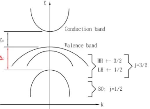
Figure 4.1. Qualitative sketch of the band structure of GaAs close to the fundamental gap.

profound e¤ect on the energy band structure En(k). For example, in

semiconduc-tors such as GaAs, SO interaction gives rise to a splitting of the topmost valence band,see Fig. 4.1.

In a tight-binding picture without spin, the electron states at the valence band edge are p-like (orbital angular momentum l = 1). With SO coupling taken into account, we obtain electronic states with total angular momentum j = 3=2 and j = 1=2. These j = 3=2 and j = 1=2 states are split in energy by a gap 0, which

is referred to as the SO gap.

This example illustrates how the orbital motion of crystal electrons is a¤ected by SO coupling. (We use the term "orbital motion" for Bloch electrons in order to emphasize the close similarity we have here between atomic physics and solid-state physics.) It is less obvious in what sense the spin degree of freedom is a¤ected by the SO coupling in a solid. Here we shall analyze both questions for quasi-two-dimensional semiconductors such as quantum wells (QWs) and heterostructures.

50 It was …rst emphasized by Elliot [37] and by Dresselhause et al. [38] that the Pauli SO coupling, Eq. 4.1 , may have important consequences for the one-electron energy levels in bulk semiconductors. Subsequently, SO coupling e¤ects in a bulk zinc blende structure were discussed in two classic papers by Parmenter [39] and Dresselhause [40]. Unlike the diamond structure of Si and Ge, the zinc blende structure does not have a center of inversion, so that we can have a spin splitting of the electron and hole states at nonzero wave vectors k even for a magnetic …eld B = 0. In the inversion-symmetric Si and Ge crystals we have, on the other hand, a twofold degeneracy of the Bloch states for every wave vector k. Clearly, the spin splitting of the Bloch states in the zinc blende structure must be a consequence of SO coupling, because otherwise the spin degree of freedom of the Bloch electrons would not know whether it was moving in an inversion-symmetric diamond structure or an inversion-asymmetric zinc blende structure.

In the solid-state physics, it is a considerable task to analyze a microscopic Schrödinger equation for the Bloch electrons in a lattice-periodic crystal potential. (We note that in a solid (as in atomic physics) the dominant contribution to the Pauli SO term, Eq. 4.1, stems from the motion in the bare Coulomb potential in the innermost region of the atomic cores. In a pseudopotential approach the bare Coulomb potential in the core region is replaced by a smooth pseudopotential.) Often, band structure calculations for electron states in the vicinity of the funda-mental gap are based on the k p method and the envelope function approximation (EFA). Here SO coupling enters solely in terms of matrix elements of the operator,