利用範例中斷點距離建構基因體規模的演化樹之研究

全文

(1)國立交通大學. 生物資訊所碩士論文. 根據模範中斷點距離建構基因體間的演化關係 On the Study of Reconstructing Genome-scale Phylogenetic Tree Based on Exemplar Breakpoint Distance. 研究生：林光倫指導教授：盧錦隆. 教授. 中華民國九十六年六月.

(2) 利用範例中斷點距離建構基因體規模的演化樹之研究 On the Study of Reconstructing Genome-scale Phylogenetic Tree Based on Exemplar Breakpoint Distance. 研究生：林光倫指導教授：盧錦隆. Student：Kuang-Lun Lin 教授. Advisor：Prof. Chin Lung Lu. 國立交通大學生物資訊所碩士論文. College of Biological Science and Technology National Chiao Tung University in partial Fulfillment of the Requirements for the Degree of Master in Biological Science and Technology June 2007 Hsinchu, Taiwan, Republic of China. 中華民國九十六年六月.

(3) 利用範例中斷點距離建構基因體規模的演化樹之研究. 學生：林光倫. 指導教授：盧錦隆. 教授. 國立交通大學生物科技學系生物資訊所碩士班. 摘要隨著 DNA 定序技術的進步，越來越多物種的完整基因體序列變得更容易取得。因此，藉由比較物種基因體之間的基因次序所推測出來的基因體規模的演化樹，將有助於物種演化親屬關係的重建。在這篇論文中，我們研究如何利用兩兩物種之間基因次序的範例中斷點距離去建構出基因體規模的演化樹。給定兩組基因體之間共有基因的次序，其中每個基因出現的次數可能不只一次，對這種基因，我們可以刪除其他重複出現的地方而只保留其中一份，最後我們可以得到二組簡化的基因次序，其中每一個基因在序列中只出現一次。而所謂的範例中斷點距離被定義成在所有可能的簡化基因次序中，所得到的最小中斷點距離。在這份研究中，我們首先改進之前計算範例中斷點距離的演算法，而這個演算法是結合分支界定與個個擊破的策略所設計出來的。接著，我們實作出這個演算法並且整合其他已有程式，例如： i.

(4) INPARANOID 與 PHYLIP 等等，發展成一套網站伺服器的工具，我們稱之為 EmBeDtree。除此之外，拿一些蛋白細菌與細胞的基因體來對 EmBeDtree 作測試，並且將畫出的基因體規模演化樹和其他的方法所畫出的演化樹視為參考樹作比較，實驗結果顯示，EmBeDtree 建構出來的演化樹和參照樹之間有很高的相似度。這意味著範例中斷點距離是一個有用衡量方式，可以用來建構出物種之間的基因體規模的演化樹。. ii.

(5) On the Study of Reconstructing Genome-Scale Phylogenetic Tree Based on Exemplar Breakpoint Distance. Student: Kuang-Lun Lin. Advisor: Prof. Chin Lung Lu. Institute of Bioinformatics Department of Biological Science and Technology National Chiao Tung University. ABSTRACT As more and more complete genomes of species are available, a genome-scale phylogenetic inference by comparing gene orders between species whole genomes can be useful for the reconstruction of the evolutionary relationships of species. In this thesis, we study the reconstruction of such genome-scale phylogenetic trees based on pairwise exemplar breakpoint distances between gene orders of species. Given the orders of multiple genes shared by two species genomes, the so-called exemplar breakpoint distance between two gene orders of two genomes is the smallest breakpoint distance between their reduced genomes that are obtained by deleting redundant copies of each gene in species genomes. In this study, we first modify a previous algorithm that is a combination of branch-and-bound and divide-and-conquer approaches to calculate the pairwise exemplar breakpoint distance. We then implement this algorithm as a web server, called EmBeDtree, by incorporating other iii.

(6) programs, such as INPARANOID and PHYLIP. EmBeDtree takes as the input multiple species genomes and outputs a phylogenetic tree based on the pairwise exemplar breakpoint distances. In addition, we test our EmBeDtree by using some data sets of Proteobacterial genomes and cellular genomes and also compared their genome trees produced by our EmBeDtree with those reference trees created by other different approaches. The experimental results show that our genome trees are greatly consistent with the trees that were constructed by other approaches, suggesting that exemplar distance is a useful measure for the reconstruction of genome-scale phylogenetic tree.. iv.

(7) 誌. 謝. 首先要感謝我的家人，有你們的栽培及鼓勵，才讓我得以無憂無慮地攻讀碩士學位。謝謝在我身邊的朋友、同學們，有你們的陪伴，使我得以在繁忙之餘得以放鬆心情，繼續向前進。謝謝實驗室的學姊、同學、學弟們，有你們互相討論與激勵，使我每每在研究上遇到困難時，得以突破瓶頸。最後感謝我的指導老師盧錦隆教授，時時督導我要認真努力作研究，讓我得以順利畢業。. v.

(8) Contents Chinese Abstract. i. Abstract. iii. Acknowledgement. v. List of Figures. viii. 1. Introduction. 1. 2. Preliminaries. 5. 2.1 Orthology and Paralogy ……………………………………. 5. 2.2 INPARANOID ……………………………………………... 9. 2.3 The Exemplar Breakpoint Distance Problem …………….... 10. 3. Method and Implementation. 13. 3.1 Algorithm …………………………………………………… 13 3.2 Implementation of EmBeDtree Web Server ………………… 20. 4. Experiments and Discussion. 26. 4.1 An Experiment of 12 Gamma-Proteobacterial Genomes …... 26. vi.

(9) 4.2 An Experiment of 18 Porteobacteria Genomes …………….. 32. 4.3 An Experiment of Cellular Genomes ……………………… 34 4.4 An Experiment of 4 Vibrio Genomes ……………………… 38. 5. Conclusion and Future Works. 40. References. 41. vii.

(10) List of Figures 2.1 A hypothetical phylogenetic tree illustrating orthologous and paralogous relationships in three species. ………………….. 7. 2.2 Effect of HGT on orthology. Gene XB in species B is acquired by HGT from gene XC in species C. ……………………… 8 3.1 The flow char of our approach. ……………………………. 14. 3.2 The partial table of horizontally transferred genes in Escherichia coli K12 that were maintained in the HGT-DB database. ………………………………………………….... 15. 3.3 The numbers of ORFs of 12 gamma-Protebacterial genomes, as well as the numbers of those ORFs that are not hypothetical or putative. …………………………………………………… 16 3.4 The modified Sankoff-Nguyen’s algorithm. ………………. 18. 3.5 The interface of EmBeDtree. …………………………….... 23. 4.1 The reference tree proposed by Lerat et al. based on the concatenation of 205 proteins. …………………………….. 28. 4.2 The genome tree reconstructed by EmBeDtree. …………... 29. 4.3 The genome tree constructed by Blin et al. based on their defined breakpoint distances. ……………………………... 30. 4.4 The genome tree constructed by Blin et al. based on their defined common interval distances. ………………………. 31. 4.5 The genome tree constructed by Blin et al. based on their defined conserved interval distances. ……………………. viii. 32.

(11) 4.6 The genome tree constructed by EmBeDtree for the complete genomes of 3 alpha-Proteobacteria, 3 beta-Protebacteria and 12 gamma-Proteobacteria, correctly clustering these Proteobacteria as three monophyletic clades. …………………………… 4.7 The genome tree constructed based on 16s RNA sequence.. 34 36. 4.8 The genome tree constructed by Snel et al. based on gene content between genomes. ……………………………...... 37. 4.9 The genome tree reconstructed by EmBeDtree, where we re-drew this EmBeDtree as an unrooted tree for the purpose of comparing it with the genome tree in Figure 4.8 and 4.9. .... 38. 4.10 The genome tree reconstructed by EmBeDtree for 4 Vibrio genomes, correctly showing that V. vulnificus YJ016 and V. vulnificus CMCP6 are in a sister group and that V. vulnificus is closer to V. parahaemolyticus than to V. cholerae. ................ ix. 39.

(12) Chapter 1 Introduction The increasing availability of complete genome sequences provides biologists a valuable dataset to reconstruct the evolutionary relationships of species through genome-scale phylogenetic inference. During evolutionary process, species genomes are subject to genome rearrangements (e.g., reversals and transpositions) that alter the ordering and orientation of genes on the chromosomes. Compared to point mutations (e.g. base substitutions, insertions and deletions), these events of genome rearrangements are relatively rare, potentially giving biologists valuable information for inferring those ancient events that occurred in the evolutionary history of species. Thus far, many approaches of analyzing genome rearrangements on the basis of gene orders of whole genomes have been increasingly used and also proved to be powerful for the phylogenetic study of both prokaryotes and eukaryotes [1, 18]. Most of these algorithms, however, has been restricted to the case where each considered gene in on genome is orthologous to exactly one gene in the other genome (i.e., one-to-one orthologs), where orthologs are homologous genes derived by a speciation event [12]. However orthology is not necessarily a one-to-one relationship, because 1.

(13) lineage-specific gene duplications can produce the so-called inparalogs that are also considered as a kind of orthologs, leading the orthologous relationship. between. species. genomes. to. be. one-to-many. or. many-to-many [12]. Note that paralogs are those homologous genes that arose by gene duplication events and currently they are further divided into two subtypes that are outparalogs and inparalogs, where outparalogs are those paralogs that were duplicated before a given speciation event under consideration, and inparalogs are those paralogs that were duplicated after the speciation event [12, 21]. To utilize the currently existing algorithms for analyzing such genomes containing inparalogs, biologists are often forced to reduce the gene contents of their genomes by deleting all gene families with inparalogs. Such a compromise seems to work well in phylogenetic reconstruction for simple genomes, such as viral and mitochondrial genomes, whereas it shall inevitably result in the consequent loss of accuracy for more complex genomes, such as prokaryotic and eukaryotic genomes, due to artificial loss of data. Sankoff [4] first addressed the above issue, when he studied the genome rearrangement problem between two genomes with multiple gene families, and formulated a general version of this problem, which aims at deleting all but one member of each gene family (where the remaining gene in each family is then called true exemplar and the reduced genomes are called exemplar genomes simply) in each of the two genomes being compared so as to minimize some rearrangement distance (e.g., breakpoint or reversal distance) between the two reduced genomes. The minimum breakpoint (respectively, reversal) distance required in the above problem is called as the exemplar breakpoint distance (respectively, 2.

(14) exemplar reversal distance) and simply denoted by EBD (respectively, ERD). The motivation with which Sankoff defined this generalized genome rearrangement problem came from the following assumptions. In a family of multiple genes, the true exemplar is the direct descendant of its ancestral gene and the others are the direct or indirect duplicates of the true exemplar. During the evolutionary process, all these genes can be moved by rearrangement events from their original positions to elsewhere in the genome. The true exemplars, however, will be displaced marginally less frequently than the others, cumulatively causing that the final rearrangement distance between the reduced genomes containing only the true exemplars in the two genomes is distinctly smaller than that of any other pair of reduced genomes. Currently, there is a branch-and-bound algorithm, proposed by Sankoff [4], to solve the exemplar breakpoint distance problem. However, this branch-and-bound algorithm requires exponential time to complete its computation for some large instances. In fact, Bryant [3] has proved this problem to be NP-hard, implying that it is unlikely to have a polynomial-time algorithm to solve this problem. Recently, Nguyen et al. [20] have further utilized the divide-and-conquer approach to improve Sankoff’s algorithm for calculating the EBD between two gene orders. The basic idea of their approach is to partition the input set of gene families into several disjoint subsets such that two gene families in different subsets are independent, then apply Sankoff’s algorithm to each subset for calculating its EBD, and finally add all these EBDs of subsets to obtain the optimal EBD for the original input set. According to the tests 3.

(15) with both some simulated datasets and a real dataset, Nguyen et al. showed that their improved Sankoff’s algorithm indeed has better computational performance than the original one. However, it still needs a quite lot of time for those genomes whose gene families intrinsically cannot be partitioned into small or small enough subsets, because the problem as mentioned above is NP-hard. In this thesis, we study how to reconstruct a genome-scale phylogenetic tree of species (also called genome tree here) based on the distances of pairwise EBD between species whole genomes. In this study, we have utilized a modified Sankoff-Nguyen’s algorithm (as mentioned in Chapter 3 of METHOD) as the kernel to develop a tool, called EmBeDtree, for the reconstruction of such a genome tree. EmBeDtree takes as input a set of accession numbers of species genomes and outputs their genome tree, as well as the lists and orders of detected orthologous genes with one-to-many and many-to-many relationships between any pair of genomes, the distance matrix of pairwise EBDs, and so on. In addition, we have evaluated our EmBeDtree by using some data sets of Proteobacterial genomes and cellular genomes and also compared their genome trees produced by our EmBeDtree with those reference trees created by other different approaches. In Chapter 4 of EXPERIMENT, we have shown that our genome trees are greatly consistent with the trees that were constructed by other approaches, suggesting that exemplar distance is a useful measure for the reconstruction of genome-scale phylogenetic tree.. 4.

(16) Chapter 2 Preliminaries In this chapter, we shall first introduce the concept of orthology and paralogy. We shall then introduce INPARANOID [21], a program for identifying clusters of true orthologous genes with including inparalogs. Finally we shall introduce the problem of exemplar breakpoint distance that was originally defined by Sankoff [4].. 2.1. Orthology and Paralogy Walter Fitch first introduced the notions of orthologs and paralogs in. 1970 [8]. In general, orthologs are genes in different species that derived from a single gene in the last common ancestor of these species; by contrast, paralogs are genes related by duplication within a genome. A property of othologs is that they perform the same functions in the respective organisms. However paralogs perform biologically distinct. Recently, Sonnhammer et al. further classified paralogs into two subtypes: inparalogs and outparalogs [25]. Given a lineage that was separated by a speciation event from the others, inparalogs (respectively, outparalogs) are those paralogs in the given lineage that all evolved by 5.

(17) gene duplications that happened after (respective, before) the speciation event. For instance, Figure 2.1 shows a hypothetical tree illustrating orthologous and paralogous including outparalogous and inparalogous relationships in three species. The phylogenetic tree consists of three branches, each forming a distinct case of orthologous-paralogous relationships. This hypothetical scenario starts with three genes (X, Y and Z) that are outparalogs relative to the speciation event. Branch 1 illustrates a straightforward case that the three species (A, B and C) inherit vertically XA, XB, XC rom that last common ancestor. Then, the three genes in different species are orthologous to each other, and they show a one-to-one orthologous relationship. Branch 2 shows additionally that a lineage-specific duplication in species A. Because the duplication occurred after the speciation event, gene YA1 and gene YA2 are called inparalogs. Moreover, genes YA1 and YA2 are also orthologs of genes YB and YC, and they show one-to-many orthologous relationships. In branch 3, a more complex evolutionary scenario emerges by duplications in each species. By definition, gene ZC1 and gene ZC2 are inparalogs as well as ZB1 and ZB2, and ZC1, ZC2 and ZC3, and they show many-to-many orthologous relationships.. 6.

(18) Figure 2.1: A hypothetical phylogenetic tree illustrating orthologous and paralogous relationships in three species (adapted from [5]).. Horizontal gene transfer (HGT), the transfer of genes between different species, is recognized as one of the major forces in prokaryotic genome evolution [11]. It was reported that HGT might cause a problem in the determination of orthologous and paralogous relationships [5]. For example, as shown in Figure 2.2, species A and B may have homologous genes XA and XB, where gene XA is ancestral but gene XB has been acquired via HGT from an outside species C. This situation is called xenologous gene displacement (XGD) by Gray GS et al. [10]. In a 7.

(19) careless analysis, XA and XB would be considered as orthologs. However, these two genes are not orthologs by definition, because they do not come from an ancestral gene in the last common ancestor of the compared species. In prokaryotic genomes, such confusion caused by HGT is very common.. Figure 2.2: Effect of HGT on orthology. Gene XB in species B is acquired by HGT from gene XC in species C.. With a rapid enrichment of genome sequences, how to identify orthologs and paralogs between different genomes becomes an important task. The simple assumption is that the sequences of orthologous genes should be more similar to each other than with any other genes in the compared genomes. This assumption suggests an approach, called symmetrical best hits (SymBets), for identifying the orthologous genes between two whole genomes. The relation of gene a in genome A and gene b in genome B is called symmetrical best hits, if gene a is the most similar to gene b than any other gene in genome B, and vice versa. On the 8.

(20) other hand, there are several approaches proposed to detect and cluster probable orthologs including inparalogs between different species, such as COG [22, 26] and INPARANOID [21]. In this study, we shall utilize INPARANOID in identifying the orthologous genes with inparalogs between two given genomes.. 2.2. INPARANOID Remm et al. [21] proposed an automatic method for finding. orthologs with inparalogs from two species genomes and developed a program, called INPARANOID. Based on their algorithm, the methodology, as described as follows, can be seen as an extension of the all-versus-all technique based on BLAST search. Given two species genomes, the first step of INPARANOID is to run BLAST search between all pairs of gene sequences. Consequently, the pairs with similarity scores above the predefined threshold are reserved for further analyses on the next step. Next, INPARANOID continues to find two-way best hits (i.e., SymBets) as potential orthologs and further include inparalogs to form putative orthologous groups, based on the idea that the main ortholog has more similarity to inparalogs from the same species than to any sequence from another species. Third, INPARANOID applies a clustering algorithm to all the putative orthologous groups as follows: (1) Merge two orthologous groups if the symmetric best orthologous genes are already clustered in the same group. 9.

(21) (2) Merge two orthologous groups if a main orthologous gene in one genome has equally best hit to two orthologous genes in the other genome. (3) Delete a new group if one of the orthologous genes already belongs to a much stronger (i.e., high similarity) group. (4) Merge two groups if one gene of the orthologous gene pair has a high similarity in another group. (5) All other overlapping groups of inparalogs are separated based on their similarity to the orthologous gene. Finally, the confidence values of a set of orthologous groups are calculated to estimate the reliability of each group (for details, we refer the reader to [21]). Currently, INPARANOID is a free program that can be accessed at http://www.cbg.ki.se/inparanoid/.. 2.3. The Exemplar Breakpoint Distance Problem We shall use the same notation as adopted in Sankoff’s paper [4] to. introduce the exemplar breakpoint distance problem. Given an alphabet A representing the gene families, let G and H be two strings (genomes) of signed (+ or -) symbols (representing genes) from A. For a symbol corresponding to a gene, all its occurrences in both genomes are said to constitute a gene family. For genomes G and H, their exemplar strings, denoted by g and h respectively, are constructed by deleting all but one occurrence of each 10.

(22) gene family in the genomes. Note that in these two exemplar strings, h is just a permutation of g. Consider two exemplar strings g = g1g2…gn and h = h1h2…hn, where n = |A| (i.e., the number of gene families). We say that gi precedes gi+1 in g for each 1≦i＜n. If gene a precedes b in g and neither a precedes b nor -b precedes -a in h, then they produce a breakpoint in g. The breakpoint distance (BD) between g and h is the number of breakpoints in g, which is also equal to the number of breakpoints in h. The exemplar breakpoint distance (EBD) between G and H is the minimum of the breakpoint distance between g and h over all choices of exemplar strings g and h from G and H, respectively. The exemplar breakpoint distance problem is defined to be the problem of finding the EBD between two given genomes G and H. For example, let G = (-2, -1, 2, 1, -3, 4, 3) and H = (1, -1, 3, 1, -3, 2, 4) be two given genomes, where gene 4 is a one-to-one orthologous gene between G and H and the others are one-to-many (e.g., gene 2) and many-to-many (e.g., genes 1 and 3) orthologous genes. Then we can delete the redundant genes in each of multiple gene families to obtain two reduced exemplar genomes g = (-2, -1, -3, 4) and h = (3, 1, 2, 4) whose breakpoint distance is 2. Note here that to calculate the breakpoint distance between g and h, it is the convention that an additional gene 0 will be added in the beginnings of g and h, and an additional gene 5 will be added in the ends of g and h. That is, in this convention, g = (0, -2, -1, -3, 4, 5) and h = (0, 3, 1, 2, 4, 5). By definition, the breakpoint distance between g and h is 2, because the two breakpoints in g are (0, -2) and (-3, 11.

(23) 4). It is not hard to verify that the breakpoint distance between g and h is the minimum over all exemplar genomes of G and H. Therefore, the EBD in this example is 2.. 12.

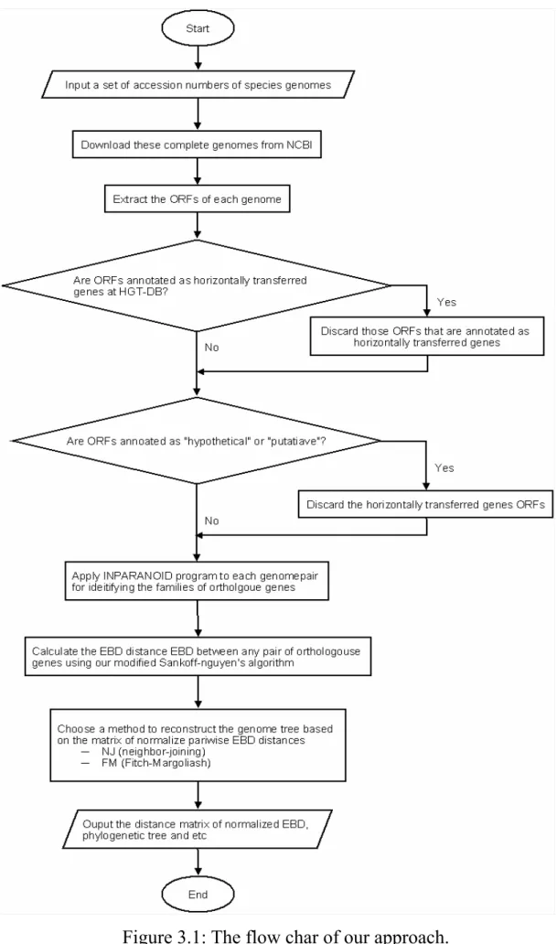
(24) Chapter 3 Method and Implementation In this chapter, we shall describe our algorithm that combines the branch-and-bound algorithm by Sankoff [4] and the divide-and-conquer algorithm by Nguyen et al. [20] for the reconstruction of genome trees based on the pairwise exemplar breakpoint distances between species whole genomes, as well as its implementation and usage of a web server EmBeDtree.. 3.1. Algorithm Figure 3.1 shows the flowchart of our method for constructing the. genome-scale phylogenetic tree based on exemplar breakpoint distance.. 13.

(25) Figure 3.1: The flow char of our approach. 14.

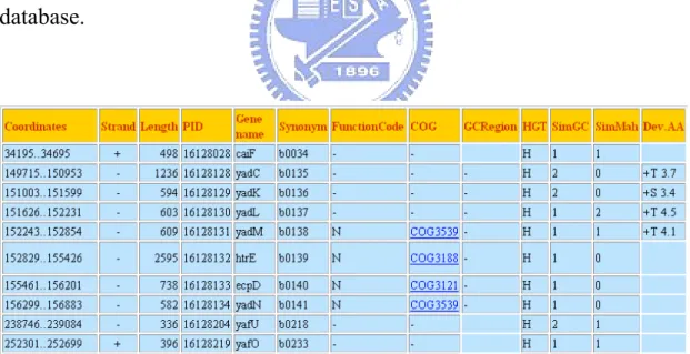
(26) Given the accession numbers of several species, the first step of our method is to download their complete genomes from NCBI [19] and extract the protein coding genes (CDS) from each genome according to the annotation of open reading frames (ORFs). For prokaryotic genomes, some of these ORFs may be acquired via HGT events that may invalidate the detection of orthologs, as discussed in Section 2.1. Currently, there is a database called HGT-DB [9] that provides the lists of putative horizontally transferred genes for a number of prokaryotic complete genomes. For example, Figure 3.2 shows the partial table of horizontally transferred genes in Escherichia coli K12 in the HGT-DB database. Hence, for bacterial and archaeal genomes, we further remove those ORFs that are annotated as horizontally transferred genes in the HGT-DB database.. Figure 3.2: The partial table of horizontally transferred genes in Escherichia coli K12 that were maintained in the HGT-DB database.. In addition, we further remove those ORFs that are annotated as “hypothetical” or “putative” ORFs. It should be noticed that for some 15.

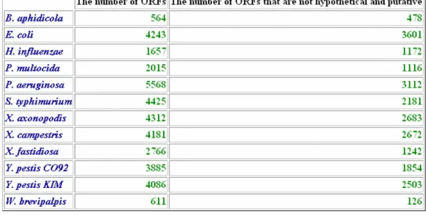
(27) species, most of their ORFs are currently annotated to be hypothetical or putative, because their genomes are not characterized well so far. Figure 3.3 shows the numbers of ORFs of 12 gamma-Protebacterial genomes, particularly in which a great number of ORFs in W. brevilpalpis are currently annotated as hypothetical or putative ORFs.. Figure 3.3: The numbers of ORFs of 12 gamma-Protebacterial genomes, as well as the numbers of those ORFs that are not hypothetical or putative.. Next, we apply the INPARANOID program [21] to each genome pair for identifying the families of orthologous genes with one-to-many and many-to-many relationships. We then parse the INPARANOID output file and assign a specific gene family number to each orthologous group that corresponds to a gene family. It should be noticed that a gene number may occur many times in the gene order of each genome, because the orthologous groups identified by INPARANOID may include 16.

(28) inparalogs.. Third, we calculate the distance of EBD between any pair of orthologous gene orders. Basically, we can utilize the divide-and-conquer approach proposed by Nguyen et al. [20] for the computation of EBD. Recall here that the basic idea of this divide-and-conquer approach is to partition the input set of gene families into several disjoint subsets such that two gene families in different subsets are independent, then apply Sankoff’s algorithm to each subset for calculating its EBD, and finally add all these EBDs of subsets to obtain the optimal EBD for the original input set. In [20], Nguyen et al. have also mentioned an approximation method to obtain an upper bound, as well as a lower bound, of the optimal EBD. The method is to directly remove some gene families from the input dataset such that the remaining gene families can be partitioned into small enough subsets. According to our experiments with real bacterial genomes, the upper bounds of their EBDs obtained by the Nguyen’s approximation method can be very close to the optimal ones, and more often, they are better than those obtained by the greedy method used in the Sankoff’s branch-and-bound algorithm for the finding of the initial upper bound. This inspires us to further incorporate this approximation method into our modified Sankoff-Nguyen’s algorithm, as shown in Figure 3.5, for finding its initial upper bound of EBD, so that a great number of unnecessary branches of the solution space can be pruned in the running of our modified Sankoff-Nguyen’s algorithm and hence its overall performance can be further speeded up.. 17.

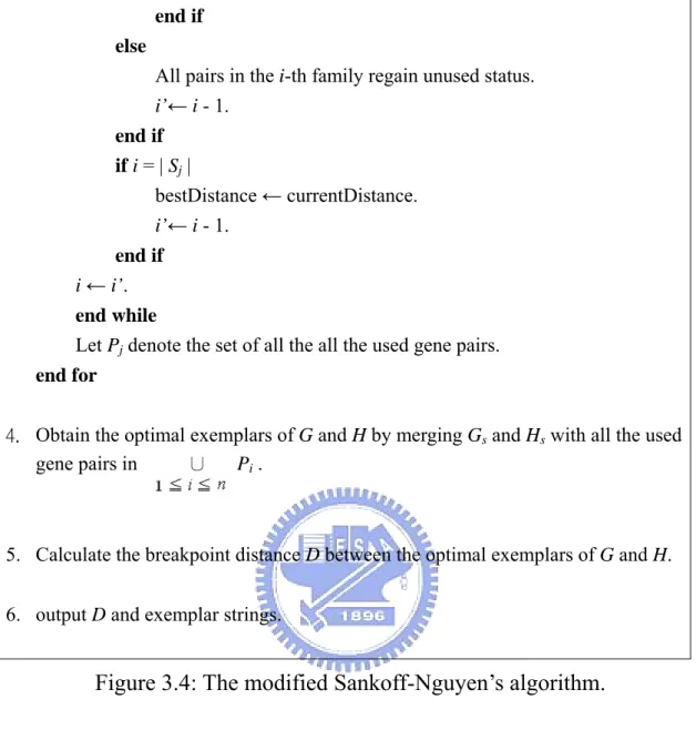
(29) Algorithm: Computation of EBD input: genomes G and H. output: exemplar breakpoint distance D between G and H. 1. Form partial exemplars of G and H, say Gs and Hs, respectively, with all the gene families with one-to-one orthologous relationship. 2. Divide gene families with one-to-many or many-to-many orthologous relationship into disjoint subsets S1…Sn that are independent with respect to Gs and Hs. The definition of independency between two gene families is proposed by Nguyen et al. For details, we refer the reader to []. 3. for each disjoint subset Sj In all families in Sj, all pairs of genes that come from G and H, respectively, are initially unused. i ← 0. bestDistance ← The upper bound of Sj obtained by the approximation method proposed by Nguyen et al. currentDistance ← 0 while i ≧ 0 if there remain unused pairs in the i-th family if all the pairs in the i-th family are unused For each pair, evaluated cumulative distance d between the partial exemplar strings constructed by inserting this pair into the two partial exemplar strings based on the first i - 1 families. end if Expand the partial exemplar strings by inserting the unused pair with minimal d. This pair acquires “used” status. if ( d + currentDistance ) ≧ bestDistance All pairs in the i-th family regain unused status. i’← i - 1. else currentDistance ← currentDistance + d. i’← i + 1. 18.

(30) end if else All pairs in the i-th family regain unused status. i’← i - 1. end if if i = | Sj | bestDistance ← currentDistance. i’← i - 1. end if i ← i’. end while Let Pj denote the set of all the all the used gene pairs. end for 4. Obtain the optimal exemplars of G and H by merging Gs and Hs with all the used gene pairs in ∪ Pi .. 5. Calculate the breakpoint distance D between the optimal exemplars of G and H. 6. output D and exemplar strings.. Figure 3.4: The modified Sankoff-Nguyen’s algorithm. Note that, for our purpose, the distance between each pair of orthologous gene orders computed by our modified Sankoff-Nguyen’s algorithm is normalized by dividing the total number of the orthologous genes shared by the two genomes. Finally, we reconstruct a phylogenetic tree from the distance matrix of the normalized pairwise EBDs. Currently, NJ (neighbor-joining) [23] and FM (Fitch-Margoliash) [7] are the most widely used methods for the creation of phylogenectic tree. Hence, we utilize these two methods, both of which have been implemented in the PHYLIP package [6], to 19.

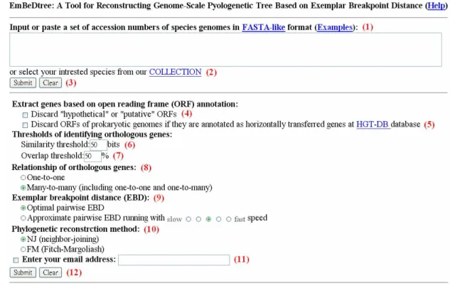
(31) reconstruct our phylogenetic tree. In addition, we use some tools in PHYLIP, such as “retree” (that can reroot and rearrange a tree), “drawgram” (that can draw a rooted tree and save it as a picture file) and “drawtree” (that can draw an unrooted tree as a picture file), to draw our computed genome tree.. 3.2. Implementation of EmBeDtree Web Server The kernel programs of EmBeDtree (EmBeDtree web server is at. http://Bioalgorithm.life.nctu.edu.tw/EmBeDtree ) were written in C, C++, Perl and its web interface was implemented in PHP. It is available for online analysis and can be easily accessed via a simple web interface (see Figure 3.5). The input of EmBeDtree is as followed: 1. Enter or paste a set of accession numbers of species genomes in FASTA-like format (1), or simply select them from our COLLECTION (2), in which there are currently 27 Archaeal genomes, 329 Bacterial genomes and 18 Eukaryal genomes. Note that EmBeDtree will automatically download the complete genomes of the input species from the NCBI. Here are some examples of FASTA-like format: Examples 1: 12 gamma-Proteobacterial genomes >BAp NC_002528 >eco NC_000913 >hin 20.

(32) NC_000907 >pmu NC_002663 >pae NC_002516 >stm NC_003197 >xac NC_003919 >xcc NC_003902 >xfa NC_002488 >ype NC_003143 >ypk NC_004088 >wgl NC_004344. Examples 2: 4 Vibrio genomes (note that the genomes of the two input chromosomes in each Vibrio species will be concatenated together according to their input order) >V. vulnificus YJ016 NC_005139, NC_005140 >V. vlunificus CMCP6 NC_004459, NC_004460 >V. parahaemolyticus RIMD 2210633 NC_004603, NC_004605 >V. cholerae E1 Tor N16961 NC_002505, NC_002506. 2. Just click “Submit” button if the user would like to run EmBeDtree with default parameters; otherwise, the user continues with the following parameter settings. 3. Check the box in (4) if the user would like to discard those 21.

(33) genes that are annotated as “hypothetical” or “putative” in the downloaded genome. 4. Check the box in (5) if the user would like to discard those genes of prokaryotic genomes that are already annotated as horizontally transferred genes at the HGT-DB database. 5. Specify the thresholds of identifying orthologous genes, including similarity threshold (6) whose default is 50 bits and overlapping threshold (7) whose default is 50%. 6. Determine the relationship of detected orthologous genes (8), which can be either one-to-one or many-to-many (also including one-to-one and one-to-many). The default is many-to-many. 7. Choose either optimal or approximate pariwise EBD (Exemplar Breakpoint Distance) to be computed (9). The default is to compute the optimal EBD. If the approximate EBD is chosen, the user can further select the speed of executing EmBeDtree, which can be slow of fast. In fact, there is a trade-off between the accuracy of the computed approximate EBD and the execution speed of EmBeDtree: the higher the execution speed of EmBeDtree, the worse the accuracy of the computed approximate EBD (i.e., the gap between the computed approximate EBD and the optimal EBD becomes larger). 8. Choose the distance-based method of reconstructing the phylogenetic tree (10) based on the distance matrix of the computed optimal/approximate pairwise EBDs between 22.

(34) genomes. It can be either NJ (neighbor-joining) that is the default or FM (Fitch-Margoliash). 9. Check the email box and simultaneously enter an email address (11), if the user would like to run EmBeDtree in a batch way. In this way, the user will be notified of the output via email when the submitted job is finished. This email check is optional but recommended, because it is still time-consuming for running EmBeDtree if the number of genomes the user entered is large, or some of the input genomes are large-scale. 10. Click “Submit” button to run EmBeDtree (12).. Figure 3.5: The interface of EmBeDtree.. In the output page, EmBeDtree will show the following information 23.

(35) in detail: z A list of the user-defined parameters. z A distance matrix of normalized pairwise EBDs computed by EmBeDtree, along with a link to a text file of this distance matrix in the PHYLIP format. Note that in this distance matrix, Each diagonal entry shows the number of protein-coding. genes. extracted. from. the. corresponding species genome, with a link to show the detailed information of these genes, e.g., gene ID, Gi, protein ID, gene name, locus-tag, start and end positions for each gene on the genome, and strand of gene on the chromosome; The entry in the upper-right triangle shows the number of identified orthologous genes in the corresponding genome pair, with a link to show the details of all orthologous pairs, e.g., for each orthologous pair, its gene numbers used in EmBeDtree, its gene strands, gene IDs and protein IDs on the genomes being considered, and its BLAST 2 alignment; The entry in the lower-left triangle shows the normalized EBD between a pair of corresponding normalized EBD computed by EmBeDtree. z The reconstructed phylogenetic tree, along with a link to its text file in Newick format. 24.

(36) Note that in the case of executing approximate EBD, the output page will show two distance matrices that contain the upper bounds of EBDs and the lower bounds of EBDs between all genome pairs, respectively, and their reconstructed phylogenetic trees. An online help page is provided in EmBeDtree to show the user how to use this web server in detail. It is worth mentioning that EmBeDtree allows the user to reconstruct the genome trees based on approximate pairwise EBDs (i.e. the lower and upper bound of EBDs) between species genomes. This function is particularly useful for the genome instances where some of their optimal pairwise EBDs cannot be completed within a reasonable time, because the user may be able to infer the partial/whole optimal tree according to the consensus of the two approximate genome trees.. 25.

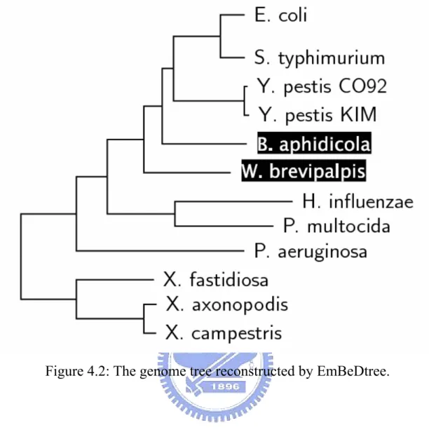
(37) Chapter 4 Experiments and Discussion In this chapter, we shall demonstrate the applicability of our EmBeDtree by carrying out experiments on four groups of genomes.. 4.1. An Experiment of 12 Gamma-Proteobacterial Genomes Here, we tested EmBeDtree with a set of 12 gamma-Proteobacterial. complete genomes studied in [2, 13], including E. coli (abbreviated as eco, NC_000913), S. typhimurium (stm, NC_003197), Y. pestis CO92 (ype, NC_003143), Y. pestis KIM (ypk, NC_004988), B. aphidicola (BAp, NC_002528), W. brevipalpis (wgl, NC_004344), H. influenzae (hin, NC_000907), P. multocida (pmu, NC_002663), P. aeruginosa (pae, NC_002516), X. fastidiosa (xfa, NC_002488), X. axonopodis (xac, NC_003919) and X. campestris (xcc, NC_003902). Using the phylogenetic tree (see Figure 4.1) propose by Lerat et al. [13] for these 12 gamma-Proteobacterial genomes (based on the concatenation of 205 proteins) as the reference tree, we compared our genome tree (see Figure 4.2) to those genome trees (see Figure 4.3, 4.4 and 4.5) reconstructed by 26.

(38) Blin et al. [2] using their defined distances based on the matching of similar segments of genes and on the notions of breakpoints, common intervals and conserved intervals. Note that our method of reconstructing the genome tree in this experiment is the same as that adopted by Blin et al. [2] that is the Fitch-Margoliash method. Intriguingly, the topology of our genome tree (as shown in Figure 4.2) was almost the same as the reference tree (as shown in Figure 4.1), with a minor exception that two endosymbionts, B. aphidicola and W. brevipalpis, were not placed in a sister group, as depicted in the reference tree, but just as neighbors in our genome tree. However, these two endosymbionts were separated in the genome trees (as shown in Figure 4.3, 4.4, 4.5) constructed by Blin et al., where B. aphidicola was close to the group of containing E. coli and S. typhimurium. In addition, P. aeruginosa was displaced as the neighbor of W. brevipalpis in their genome trees (as shown in Figure 4.4 and 4.5) based on common interval and conserved interval distances. We further used EmBeDtree to compute the approximation EBDs (i.e., upper-bounded and lower-bounded EBDs) for each genome pair in this testing dataset. Consequently, both the resulting upper-bounded and lower-bounded EmBeDtrees are equivalent to the optimal one, suggesting that the consensus between the upper-bounded and lower-bounded EmBeDtrees may equal to the optimal EmBeDtree. Notably, the computation of approximate EBD is much quicker than that of optimal EBD.. 27.

(39) Figure 4.1: The reference tree proposed by Lerat et al. based on the concatenation of 205 proteins (adapted from [13]).. 28.

(40) Figure 4.2: The genome tree reconstructed by EmBeDtree.. 29.

(41) Figure 4.3: The genome tree constructed by Blin et al. based on their defined breakpoint distances (adapted from [2]).. 30.

(42) Figure 4.4: The genome tree constructed by Blin et al. based on their defined common interval distances (adapted from [2]).. 31.

(43) Figure 4.5: The genome tree constructed by Blin et al. based on their defined conserved interval distances (adapted from [2]).. 4.2. An Experiment of 18 Porteobacteria Genomes In this experiment, we re-conducted the above experiment of 12. gamma-Proteobacterial. genomes,. but. included. additional. 3. alpha-Proteobacterial genomes that are R conorii (RiccM, NC_003103), R. prowazekii (RicpM, NC_000936) and C. crescentus (CaucC, NC_002696), and additional 3 beta-Proteobacterial genomes that are Neisseria. meningitidis. MC58. (NeimM, 32. NC_003112),. Neisseria.

(44) meningitidis Z2491 (NeimZ, NC_003116) and Neisseria gonorrhoeae (NeigF, NC_002946). Here, we show its resulting genome tree in Figure 4.6, in which the testing alpha-, beta- and gamma-Proteobacteria correctly form three monophyletic clades. Here, we also applied EmBeDtree to this dataset with the function of approximate EBD computation. As a result, both of upper-bounded EmBeDtree and lower-bounded EmBeDtree are equal to the optimal one.. 33.

(45) Figure 4.6: The genome tree constructed by EmBeDtree for the complete genomes of 3 alpha-Proteobacteria, 3 beta-Protebacteria and 12 gamma-Proteobacteria, correctly clustering these Proteobacteria as three monophyletic clades.. 4.3. An Experiment of 13 Cellular Genomes In this experiment, we tested EmBeDtree with a set of 13 complete. cellular genomes studied in [24], including A. aeolicus (AquaV, NC_000918), A. fulgidus (ArcfD, NC_000917), B. burgdorferi (BorbB, 34.

(46) NC_001318), B. subtilis (Bacss, NC_000964), E. coli (EcoliK, NC_000913), H. influenzae (HaeiR, NC_000907), H. pylori (Help2, NC_000915), M. genitalium (MycgG, NC_000908), M. jannaschii (MetjD, NC_000909), M. thermoautotrophicum (MettD, NC_000916), Synechocystis (SynsP, NC_000911), P. horikoshii (PyrhO, NC_000961), S. cerevisiae (Sacc, NC_001133, NC_001134, NC_001135). Here note that we used the genomes of the first three chromosomes of S. cerevisiae in this experiment. Using the phylogenetic tree constructed on the basis of 16s rRNA sequences (see Figure 4.7) as the reference tree, we compared our genome tree (Figure 4.9) to that (Figure 4.8) constructed by Snel et al. [24], where all these three genome trees were constructed using neighbor-joining method. Consequently, all these three genomes tree clustered the lineages of the Archaea, Bacteria and Eukarya as three monophyletic clades. In the clade of Bacteria, A. aeolicus and Synechocystis were separated in our genome tree and the reference tree, but they were placed in a sister group in the genome tree constructed by Snel et al. [24]; however, H. phylori was placed with E. coli and H. influenzae as a sister group in the reference tree and the genome tree of Snel et al., but it did not in our genome tree. In the Archaea clade, our genome tree as well as the one of Snel et al. placed M. jannaschii and M. thermoautotrophicum as a sister group, but the reference tree placed M. thermoautotrophicum and A. fulgidus instead. We further used EmBeDtree to compute the approximate EBDs between genomes in this dataset and the resulting upper-bounded EmBeDtree and lower-bounded EmBeDtree are both equivalent to the optimal one. 35.

(47) Figure 4.7: The genome tree constructed based on 16s RNA sequences (adapted from [24]).. 36.

(48) Figure 4.8: The genome tree constructed by Snel et al. [24] based on gene content between genomes (adapted from [24]).. 37.

(49) Figure 4.9: The genome tree reconstructed by EmBeDtree, where we re-drew this EmBeDtree as an unrooted tree for the purpose of comparing it with the genome trees in Figure 4.8 and 4.9.. 4.4. An Experiment of 4 Vibrio Genomes In this experiments, we used 4 pathogenic Vibrio genomes, including. V. vulnificus YJ016 (NC_005139, NC_005140), V. vulnificus CMCP6 (NC_004459,. NC_004460),. V.. parahaemolyticus. (NC_004603,. NC_004650) and V. cholerae (NC_002505, NC_002506), to test EmBeDtree. Since each of these four Vibrio pathogens consists of two chromosomes, we conducted this experiment by entering the accession numbers of the two chromosomal genomes for all Vibrio species as the 38.

(50) input of EmBeDtree. Note that in this case, the two chromosomal genomes of each Vibrio genomes were merged into a larger one for running EmBeDtree. The resulting genome tree, as illustrated in Figure 4.10, shows that V. vulnificus YJ016 and V. vulnificus CMCP6 are clustered as a sister group that V. vulnificus is closer to V. parahaemolyticus than to V. cholerae, which agrees with our previous results obtained by the approaches of analyzing Vibrio genome rearrangements based on a variety of rearrangement operations, such as block-interchanges [14, 17], block-interchanges and reversals [15] and fusions, fissions and block-interchanges [16].. Figure 4.10: The genome tree reconstructed by EmBeDtree for 4 Vibrio genomes, correctly showing that V. vulnificus YJ016 and V. vulnificus CMCP6 are in a sister group and that V. vulnificus is closer to V. parahaemolyticus than to V. cholerae.. 39.

(51) Chapter 5 Conclusion and Future Works In this thesis, we conducted the study of reconstructing genome-scale phylogenetic tree based on exemplar breakpoint distance. Our method is a combination of branch-and-bound and divide-and-conquer algorithms with a modification. Based on this approach, we have implemented a web server, called EmBeDtree, for online analysis. By several experiments, the genome trees reconstructed by our web server based on exemplar breakpoint distances are greatly consistent with the reference trees that were reconstructed by other approaches based on 16s rRNA sequences and concatenation of multiple common protein sequences. As a future work, it will be interesting to study whether the genome tress reconstructed based on other exemplar distances, such as exemplar reversal, transposition and block-interchange distances, are still consistent with the one reconstructed based on exemplar breakpoint distance and the reference trees reconstructed using other different approaches. In addition, whether two exemplar transposition and block-interchange distance problems can be solved in polynomial time are still open.. 40.

(52) References [1] Belda, E., Moya, A. and Silva, F.J. (2005) Genome rearrangement distances and gene order phylogeny in gamma-Proteobacteria, Mol Biol Evol, 22, 1456-1467 [2] Blin, G., Chauve, C. and Fertin, G. (2005) Gene order and phylogenetic reconstruction: application to gamma-Proteobacteria, Lecture Notes in Bioinformatics, 3678, 11-20. [3] Bryant, D. The complexity of calculating exemplar distance, In Comparative Genomics, (Sankoff, D. and Nadeau, J.H., eds), pp. 207-212 Kluwer Academic Publishers. [4] David Sankoff (1999) Genome rearrangement with gene families, Bioinformatics, 15, 909,917. [5] Eugene V. Koonin (2005) Orthologs, Paralogs, and Evolutionary Genomics, Annu. Rev. Genet., 39, 309-338 [6] Felsenstein, J. Phylip (phylogeny inference packate) version 3.6 Distributed by the author. Department of Genome Sciences, University of Washington, Seattle. [7] Fitch, W. M. and E. Margoliash (1967) Construction of phylogenetic trees, Science, 155, 279-284. [8] Fitch W. M. (1970) Distinguishing homologous from analogous proteins, Syst. Zool, 19, 99-106 41.

(53) [9] Garcia-Vallve, S., Guzman, E., Montero, M.A. and Romeu, A. (2003) HGT-DB: a database of putative horizontally transferred genes in prokaryotic complete genomes, Nucleic Acids Res, 31, 187-189. [10] Gray GS, Fitch WM. (1983) Evolution of antibiotic resistance genes: the DNA sequence of a kanamycin resistance gene from Staphylococcus aureus, Mol. Biol. Evol., 1, 57-66. [11] Koonin, E.V., Makarova, K.S. and Aravind, L. (2001) Horizontal gene transfer in prokaryotes: Quantification and Classification, Annu. Rev. Microbiol., 55, 709-742 [12] Koonin, E.V. (2005) Orthologs, paralogs, and evolutionary genomics, Annu Rev Genet, 39, 309-338. [13] Lerat, E., Daublin, V. and Moran, N.A. (2003) From gene trees to organismal. phylogeny. in. prokaryotes:. the. case. of. the. gamma-Proteobacteria, PLoS Biol, 1, E19. [14] Lin, Y.C., Lu C.L., Chang, H.Y. and Tang, C.Y. (2005) An efficient algorithm for sorting by block-interchanges and its application to the evolution of vibrio speices, Journal of Computational Biology, 12, 102-112. [15] Lin, Y.C., Lu, C.L., Liu, Y.C. and Tang, C.Y. (2006) SPRING: a tool for the analysis of genome rearrangements using reversals and block-interchanges, Nucleic Acids Research, 34, 696-699. [16] Lu, C.L., Huang, Y.L., Wang, T.C. and Chiu, H.T. (2006) Analysis of circular. genome. rearrangement. by. fusions,. fissions. and. block-interchanges, BMC Bioinformatics, 7. [17] Lu, C.L., Wang, T.C., Lin, Y.C. and Tang, C.Y. (2005) ROBIN: a tool. for. genome. rearrangement 42. of. block-interchanges,.

(54) Bioinformatics, 21, 2780-2782. [18] Moret, B.M.E. and Warnow, T. (2005) Advances in phylogeny reconstruction from gene order and content data, Methods Enzymol, 395, 673-700. [19] National. Center. of. Biotechnology. Information,. http://www.ncbi.nlm.nih.gov [20] Nguyen, C.T., Tay, Y.C. and Zhang, L. (2005) Divide-and-conquer approach for the exemplar breakpoint distance, Bioinformatics, 21, 2171-2176. [21] Remm, M., Storm, C.E. and Sonnhammer, E.L. (2001) Automatic clustering of orthologs and in-paralogs from pairwise species comparisons, J Mol Biol, 314, 1041-1052. [22] Roman L. Tatusov, Michael Y. Galperin, Darren A. Natale an Eugene V. Koonin (2000) The COG database: a tool for genome-scale analysis of protein function and evolution, Nucleic Acids Research, 28, 33-36 [23] Saitou, N. and Nei., M. (1987), The neighbor-joining method: a new method for reconstructing phylogenetic trees, Mol. Evol. Biol, 4,406-425 [24] Snel, B., Bork, P. and Huynen, M.A. (1999) Genome phylogeny based on gene content, Nat Genet, 21, 108-110. [25] Sonnhammer EL, Koonin EV. (2002) Orthology, paralogy and proposed classification for paralog subtypes, Trend Genet, 18, 619-620. [26] Tatsov RL, Koonin EV, Lipman DJ. (1997) A genomic perspective on protein families, Science, 278, 631-37. 43.

(55)