提昇型離散小波轉換之研究及其在影像壓縮中之應用

全文

(1)國立交通大學電機與控制工程研究所博. 士. 論. 文. 提昇型離散小波轉換之研究及其在影像壓縮中之應用 A STUDY OF LIFTING-BASED DISCRETE WAVELET TRANSFORM AND ITS APPLICATIONS IN IMAGE COMPRESSION. 研究生：蘇建焜指導教授：林昇甫教授. 中華民國九十七年七月.

(2) 提昇型離散小波轉換之研究及其在影像壓縮中之應用研究生：蘇建焜. 指導教授：林昇甫教授. 國立交通大學電機與控制工程研究所. 摘. 要. 繼離散型餘弦轉換 (discrete cosine transform; DCT) 被廣泛應用於影像壓縮領域之後，離散型小波轉換 (discrete wavelet transform; DWT) 是目前學術界和工業界研究、發展的重點，並且已經被新一代的靜態影像壓縮標準 (如 JPEG2000) 和動態影像壓縮標準 (如 MPEG-4，H.264/AVC) 所採用。早期的離散型小波轉換其實現方式是基於迴旋計算 (convolution-based) 方式，而新一代的離散型小波轉換其實現方式是所謂提昇型(lifting-based) 。「提昇型離散小波轉換」 (lifting-based DWT)具有計算效率高、節省記憶空間、可執行整數至整數小波轉換、適合平行處理，以及在某些場合無邊界延伸的問題等優點。又因其使用上非常具有彈性，所以目前仍然是大家研究的重點。本論文首先討論方向適應型離散小波轉換 (direction-adaptive DWT) ，然後提出應用於任意形狀物體影像的提昇式形狀適應型離散小波轉換 (lifting shape-adaptive DWT)，以及可以應用於任意形狀影像、且具方向適應性的形狀方向適應型離散小波轉換 (shape-direction-adaptive DWT；SDA-DWT)。由實驗結果得知本論文提出的新方法除了保有提昇型離散小波轉換的優點之外，因為具有形狀及方向上的適應性，故可以在有限的代價上獲得影像壓縮效能的顯著提昇。除此之外我們也討論結合提昇型離散小波轉換 (lifting-based DWT) 和向量量化 (vector quantization; VQ) 來改善影像壓縮效率的一些方法。 i.

(3) A STUDY OF LIFTING-BASED DISCRETE WAVELET TRANSFORM AND ITS APPLICATIONS IN IMAGE COMPRESSION Student: Chien-Kun Su. Advisor: Prof. Sheng-Fuu Lin. Department of Electrical and Control Engineering National Chiao Tung University. Abstract After the discrete cosine transform (DCT) was widely used in image compression, discrete wavelet transform (DWT) was the new dominated transform for research and industrial applications, and it has been adopted in the new still-image compression standards (e.g. JPEG2000) and video compression standards (e.g. MPEG-4 and H.264/AVC). In literature, the realization of DWT was convolution-based in early days, and for better computation efficiency, saving memory space, integer-to-integer transform, parallel processing, and boundary extension problem the lifting-based DWT was proposed later. Lifting-based DWT is still an important research topic, since it is more flexible than the convolution-based DWT to adopt new functionalities. In this dissertation, the lifting-based DWT was studied, and a lifting-based direction-adaptive DWT was discussed. Then, the lifting-based shape-adaptive DWT (LSA-DWT) and the lifting-based shape-direction-adaptive DWT, which was adaptive in shape and direction, were proposed. Because SDA-DWT has the adaptabilities of shape and direction, by paying affordable cost, we can achieve superior improvement in image compression. Beside lifting-based SA-DWT and SDA-DWT, the combination of lifting-based DWT and vector quantization (VQ) was discussed in the dissertation. ii.

(4) 誌. 謝. 感謝指導教授及師母多年來的諄諄教誨，謝謝口試委員在盛夏溽暑百忙中撥冗為我口試。謝謝所有電控系、所和交大其他系、所、單位，直接或間接教導、幫助過我的師長和小姐、先生們，也要謝謝辛錫進教授（國立聯合大學）和高川原教授（中華大學）的協助，以及實驗室內歷屆學長和學弟的幫忙。同時感謝父母的照顧和太太的包容，還有小女、小犬對我精神上的激勵。引用陳之藩先生的話：「太多人要感謝，不如就謝天吧！」. iii.

(5) CONTENTS. ABSTRACT (CHINESE). i. ABSTRACT (ENGLISH). ii. ACKNOWLEDGEMENTS (CHINESE). iii. CONTENTS. iv. LIST OF TABLES. vii. LIST OF FIGURES. viii. SYMBOL LIST. xii. CHAPTER 1 INTRODUCTION................................................................................... 1 1.1 DISCRETE WAVELET TRANSFORM ......................................................................... 2 1.2 THE APPLICATIONS AND LIMITATIONS OF CONVENTIONAL DWT.......................... 5 CHAPTER 2 LIFTING-BASED DISCRETE WAVELET TRANSFORM ............. 7 2.1 MATHEMATICAL THEORIES OF LIFTING-BASED DWT ........................................... 7 2.1.1 Filters and Laurent polynomials ................................................................... 11 2.1.2 Discrete wavelet transform in FIR form........................................................ 14 2.1.3 The lifting structure ....................................................................................... 18 2.1.4 The Euclidean algorithm ............................................................................... 21 2.1.5 The factoring algorithm................................................................................. 23 2.2 REALIZATION OF LIFTING-BASED DISCRETE WAVELET TRANSFORM ................... 26 2.2.1 Haar wavelets ................................................................................................ 26 2.2.2 The 5/3 wavelets ............................................................................................ 28 2.2.3 The 9/7 wavelets ............................................................................................ 29 2.3 LIFTING-BASED DIRECTION-ADAPTIVE DWT (DA-DWT).................................. 31 2.4 SHAPE-ADAPTIVE DWT (SA-DWT) ................................................................... 35. iv.

(6) CHAPTER 3 TWO WAVELET-BASED HYBRID CODECS FOR IMAGE COMPRESSION .......................................................................................................... 37 3.1 IMAGE COMPRESSION USING SPIHT AND VQ ..................................................... 37 3.1.1 Overview of SPIHT........................................................................................ 38 3.1.2 Proposed hybrid coding................................................................................. 39 3.1.3 Wavelet tree classification............................................................................. 41 3.1.4 MVQ Coding for High Frequency Wavelet Trees ......................................... 41 3.1.5 MVQ codebook generation ............................................................................ 42 3.1.6 Hybrid image coding ..................................................................................... 43 3.1.7 Experimental results and conclusions ........................................................... 45 3.2 IMAGE COMPRESSION BASED ON SET-PARTITIONING EMBEDDED BLOCK CODER AND RESIDUAL VECTOR QUANTIZATION .............................................................. 48. 3.2.1 Set-partitioning embedded block coder (SPECK) ......................................... 48 3.2.2 Residual vector quantization (RVQ).............................................................. 55 3.2.3 The Proposed Hybrid Image Compression Method ...................................... 57 3.2.4 Experimental results and conclusions ........................................................... 59 CHAPTER 4 THE PROPOSED METHODS ............................................................ 65 4.1 LIFTING-BASED SHAPE-ADAPTIVE DWT (LSA-DWT) ....................................... 69 4.2 SHAPE-DIRECTION-ADAPTIVE DWT (SDA-DWT) ............................................. 71 4.2.1 Illustrations of SDA-DWT ............................................................................. 72 4.2.2 Filter direction determination in SDA-DWT ................................................. 78 4.2.3 The importance of shape-adaptive and direction-adaptive functionalities in object-based image compression.................................................................. 78 CHAPTER 5 EXPERIMENTAL RESULTS OF SDA-DWT .................................. 81 5.1 OBJECT IMAGE COMPRESSION ............................................................................. 81 5.2 REGULAR IMAGE COMPRESSION .......................................................................... 87 CHAPTER 6 CONCLUSIONS ................................................................................... 93. v.

(7) REFERENCES………………………………………………………………………95 VITA………………………………………………………………….………………98 PUBLICATION LIST……………….………………………………………………99. vi.

(8) LIST OF TABLES. Table 3.1 The results of SPECK and the proposed method for 3 test images…….........61 Table 5.1 The bit numbers of the bit stream of each test object image after SPECK coding. (SDA1 and SDA2 represent SDA-DWT without object partition and with object partition, respectively. SA means SA-DWT and DA is DA-DWT.)……..………………………………………………………...........83 Table 5.2 The PSNR results for lossy compression of object image 1. (Object 1 contains 30,535 pixels.).………………………………………………... .........84 Table 5.3 The PSNR results for lossy compression of object image 2. (Object 2 contains 45,012 pixels. SDA1 and SDA2 represent SDA-DWT without object partition and with object partition, respectively.)..……………… .........84 Table 5.4 The PSNR results for lossy compression of object image 3. (Object 3 contains 10,000 pixels. SDA2 represents SDA-DWT with object partition.)…..…………………………………………………………… .........84 Table 5.5 PSNR values of three method under 0.1-bpp, 0.25-bpp, 0.5-bpp, and 1.0-bpp conditions, where CD-DWT means the conventional-direction l i f t i ngDWT…………………………………………………………….. .........88. vii.

(9) LIST OF FIGURES. Figure 1.1 Example of 3-level 2-D DWT with subbands delimited by thick lines. .........4 Figure 1.2 Example of 3-level 2-D DWT and a wavelet tree in the diagonal direction ...............................................................................................................5 Figure 2.1 Block diagram of a pair of lifting steps (prediction and update steps). The x means the input signal vector, and s and d are the output subsampled smooth (low-pass) and detail (high-pass) signal vectors, respectively..............10 Figure 2.2 Block diagram of one-dimensional DWT. x is the original signal and xˆ is the reconstruction signal of x. ........................................................................15 Figure 2.3 The polyphase representation of DWT and IDWT. ......................................17 Figure 2.4 The lifting structure: A classical subband filter scheme followed by a lifting scheme which lifts the low-pass subband with the help of the high-pass subband..............................................................................................19 Figure 2.5 The dual lifting structure: A classical subband filter scheme followed by a lifting scheme which lifts the high-pass subband with the help of the low-pass subband...............................................................................................21 Figure 2.6 The forward DWT using lifting structure......................................................25 Figure 2.7 The Inverse DWT using lifting structure. .....................................................25 Figure 2.8 DWT with lifting Haar wavelet.....................................................................27 Figure 2.9 IDWT with lifting Haar wavelet. ..................................................................27 Figure 2.10 The block diagram of a DA-DWT system. .................................................32 Figure 2.11 A Direction selection example with angle θin 1-D“ hor i z ont a l ”DWT. ...........................................................................................................................33 Figure 2.12 Nine prediction directions for an odd sample in 1-D“ hor i z ont a l ”DWT. ...........................................................................................................................34 Figure 2.13 The update stage with θ= 45o. ....................................................................34. viii.

(10) Figure 2.14 The original image and alpha map of object 1: (a) the test visual object 1 with background (256-by-256), (b) the shape mask (alpha map)...................36 Figure 3.1 Rate-distortion curves of the low frequency (dotted line) and high frequency (solid line) wavelet trees of Mandrill image by using the SPIHT algorithm............................................................................................................40 Figure 3.2 Multistage VQ structure. ...............................................................................42 Figure 3.3 Block diagram of the proposed hybrid image coder by combining SPIHT and MVQ for coding the low and high frequency wavelet trees, respectively. .......................................................................................................43 Figure 3.4 Bitstream structure. .......................................................................................44 Figure 3.5 Rate-distortion curves of the test images: Mandrill, Bridge and Lena (from left to right) by using the proposed hybrid coder (dotted lines) and SPIHT (solid lines). ...........................................................................................47 Figure 3.6 Partitioning a transformed image X into sets S and I....................................49 Figure 3.7 Quadtree partition: partitioning set S into S1, S2, S3, and S4.........................49 Figure 3.8 Partitioning set I into S1, S2, S3, and a smaller I. ..........................................50 Figure 3.9 Flow chart of the SPECK algorithm. ............................................................51 Figure 3.10 The flow chart of procedure ProcessS( ).....................................................52 Figure 3.11 The flow chart of procedure ProcessI( ). ....................................................53 Figure 3.12 The flow chart of procedure CodeS( ). ........................................................54 Figure 3.13 The flow chart of procedure CodeI( )..........................................................55 Figure 3.14 The signal flow diagram of a p-stage RVQ.................................................57 Figure 3.15 The proposed hybrid image coder. ..............................................................57 Figure 3.16 Three 256×256 gray-level test images: (a) Lena, (b) Babara, (c) Goldhill..............................................................................................................60 Figure 3.17 The partition and assignment of a 4-decomposition-leveltransformed image. ................................................................................................................60 Figure 3.18 The experimental results of the gray-level image Lena. .............................63 Figure 3.19 The experimental results of the gray-level image Barbara..........................63 ix.

(11) Figure 3.20 The experimental results of the gray-level image Goldhill. ........................64 Figure 3.21 The average improvements of the proposed hybrid coder compared to the original SPECK on more test images. .........................................................64 Figure 4.1 The structure of a lifting-based one-dimensional 5/3- wavelet DWT...........66 Figure 4.2 Flow charts of lifting 1-D 5/3 wavelet DWT and IDWT: (a) DWT, (b) IDWT.................................................................................................................68 Figure 4.3 An arbitrarily shaped segment and the relation of its even and odd pixels in the prediction step of the 1-D row direction lifting-based DWT. .................69 Figure 4.4 An arbitrarily shaped segment and the relation of its even and odd pixels in the update step of the 1-D horizontal lifting-based DWT. ............................70 Figure 4.5 The subsampling result of the arbitrarily shaped segment in Figure 4.3.......71 Figure 4.6 The first prediction step of the 2-D shape-direction-adaptive DWT (θ= 45o) performed on an arbitrarily shaped segment. .............................................73 Figure 4.7 The first update step of the 2-D shape-direction-adaptive DWT (θ= 45o) performed on an arbitrarily shaped segment......................................................74 Figure 4.8 The horizontal subsampling result of Figure 4.7 in SDA-DWT. ..................74 Figure 4.9 The second prediction step of the 2-D SDA-DWT on an arbitrarily shaped segment..................................................................................................75 Figure 4.10 The second update step of the 2-D SDA-DWT on an arbitrarily shaped segment..............................................................................................................75 Figure 4.11 The vertical subsampling result of Figure 4.10 in SDA-DWT. ..................76 Figure 4.12 The flow chart of a multilevel SDA-DWT..................................................77 Figure 4.13 An 4×4 image segment and the direction that the odd samples can be predicted perfectly .............................................................................................79 Figure 5.1 The 256 × 256 gray-level object image and its shape mask with partition: (a) the test object image, (b) the mask with partition. (Object 2 contains 45,012 pixels.) ...................................................................................................82 Figure 5.2 The 128 × 128 gray-level object image and its shape mask with partition: (a) the test object image, (b) the mask with partition. (Object 3 contains 10,000 pixels.) ...................................................................................................82 x.

(12) Figure 5.3 The object-2 reconstruction images under 1.46-bpp condition: (a) the result of SDA-DWT with object partition according to Figure 5.1 (b), (b) the result of LSA-DWT. ....................................................................................85 Figure 5.4 The reconstruction object images, under 1-bpp condition: (a) the result of SDA-DWT, (b) the result of LSA-DWT.......................................................85 Figure 5.5 The reconstruction object image and the partition and direction in DA-DWT: (a) the reconstruction result under 10,000-bit condition. (b) mask partition and block directions of partition used in DA-DWT. .................86 Figure 5.6 An example of partitioning the image in Figure 2.14 (a) for regular image compression. The suitcase image is partitioned into background, the handle, and the box manually. ...........................................................................88 Figure 5.7 Reconstruction images of three methods under 1-bpp and 0.5-bpp conditions respectively, where SDA means SDA-DWT, DA is DA-DWT, and CD-DWT denotes lifting conventional-filter-direction DWT ....................89 Figure 5.8 Reconstruction images of three methods under 0.25-bpp and 0.1-bpp conditions respectively, where SDA means SDA-DWT, DA is DA-DWT, and CD-DWT denotes lifting conventional-filter-direction DWT ....................90 Figure 5.9 A 256×256 image and its partitions: (a) the original image Pentagon, (b) partitioning the image into 9 types of blocks, (c) another non-block partition..............................................................................................................91 Figure 5.10 Transformed images of Figure 5.7 (a): (a) by SDA-DWT, (b) by conventional-direction lifting DWT. (both use 5/3 wavelet and 3 decomposition levels) Note that the high-frequency subband of Figure 5.11 (a) is smoother than Figure 5.11 (b), and it means that the former transform is usually more efficient than the later...............................................................92. xi.

(13) SYMBOL LIST x. : input vector, original signal. x(n). : discrete signal sample of x. xˆ. : reconstruction signal of x. At. : transpose of matrix A. A 1. : inverse of matrix A. det(A). : determinant of matrix A. R. : field of real numbers, vector space of real numbers. Z. : field of integers, vector space of integers. GL(2, R[z, z-1]) : mathematical ring whose elements are 2×2 matrices with Laurent polynomial entries SL(2, R[z, z-1]) : mathematical ring whose elements are 2×2 matrices with determinant 1 and Laurent polynomial entries ~ h, h. : low-pass FIR filters. g , g~. : high-pass FIR filters. q(z) = a(z)/b(z) : quotient of a(z) divided by b(z). xii.

(14) r(z) = a(z) mod b(z) : remainder of a(z) divided by b(z). a(z ). : degree of Laurent polynomial a(z). bpp. : bit-per-pixel (bits used to represent one pixel). RMSE. : root-mean-square error. PSNR (dB) = 20log10(255/RMSE) : signal to noise power ratio. 2. : downsampling (subsampling) operation. 2. : upsampling operation. xiii.

(15) CHAPTER 1 INTRODUCTION Discrete wavelet transform (DWT) are widely and successfully used in many fields, especially for image compression. Since more and more new applications and requirements are emerging, some variants of discrete wavelet transform have been designed to support new functionalities of these new applications. Shape-adaptive functionality is required in object-based image compression (e.g. MPEG-4), and Li et al. [1] and Lu et al. [2] had proposed to use convention DWTs to solve this problem. Recently, the direction-adaptive functionality of DWT was discussed by Ding et al. [3] and Chang et al. [4], and they both use lifting-based structures to design DWTs which are directional adaptive and achieve very efficient results. Those instances inspired us to develop a novel method that is both shape and directional adaptive, and to well exploit the correlation of images to achieve better performance of image compression. In this dissertation, a shape-direction-adaptive lifting-based discrete wavelet transform (SDA-DWT), which is direction adaptive and can be used for arbitrarily shaped segments, is proposed. The SDA-DWT contains three major techniques: the lifting-based DWT, the adaptive directional technique, and the concept of object-based compression in MPEG-4. The conventional separable 2-D DWT can be implemented by using 1-D DWT on the horizontal and vertical directions, respectively. Therefore, for images containing large amount of non-horizontal and non-vertical line textures, the conventional DWT is not efficient for image coding, and the direction-adaptive DWT (DA-DWT) can improve the performance for such cases. On the other hand, the traditional 2-D DWT also requires the images that are going to be transformed to be rectangular and their width and height are multiples of two. Such a requirement of the conventional DWT confines its 1.

(16) applications for arbitrarily-shaped-region or object-image compression. Hence, some shape-adaptive DWTs have been proposed for solving this problem. The lifting-based DWT implements the DWT by factoring it into three lifting steps and the lifting technique simplifies hardware implementation and SDA-DWT realization. For supporting the shape-adaptive and direction-adaptive functionalities at the same time, we propose the new SDA-DWT which can handle arbitrarily shaped still images and are directional adaptive. SDA-DWT can improve energy compaction for any shaped region containing sharp edges or line-type textures, and improve the overall coding efficiency. For the application in object-based image compression, compared to the shape-adaptive DWTs proposed in [1] and [2], SDA-DWT has the advantages that it can well exploit the orientation correlation in images and it is easier to implement for using the lifting DWT. The disadvantages of SDA-DWT include that SDA-DWT needs more side information than the shape-adaptive DWTs need, and it needs extra computation for direction decision. For the application in normal size image compression, compared to direction-adaptive DWTs, SDA-DWT can handle arbitrarily shaped partition and have higher resolution to exploit the correlation hiding in shape and orientation, while the direction-adaptive DWTs only can process rectangular partition.. 1.1 Discrete Wavelet Transform Wavelet transform [5]-[8] is well known as a multiresolution analysis that provides many advantages: joint space-spatial frequency localization, clustered wavelet coefficients of significance with strong correlations between subbands, and exact reconstruction, which are truly beneficial to image compression. Discrete wavelet transform (DWT) decomposes a signal: S (n) at resolution into two components: ~ (1.1a) S 1 (n) S (k ) h (2n k ) , k. D1 (n) S (k ) g~ (2n k ), k. 2. (1.1b).

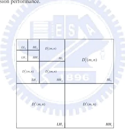
(17) where S 1 (n) is its approximation (lowpass signal) at the next coarser resolution 1 , D1 (n) is the detail information (highpass signal) between the two successive ~ resolutions: and 1 , h (n) , 1, n , g~ (n) , 1, n , ,  is an inner product operator,  is a valid (mother) wavelet,  is the scaling function that is an aggregation of wavelets at scales larger than 1, and j , n ( x) 2 j / 2 (2 j x n) . The original signal S (n) can be exactly reconstructed from S 1 (n) and D1 (n) by using the following inverse DWT (IDWT): S (n) S 1 (k ) h(n 2k ) D1 (k ) g (n 2k ), k. (1.2). k. ~ where h(n) h (n) and g (n) g~ (n) .. For image applications, the two-dimensional DWT can be obtained by using the tensor product of two one-dimensional DWT, i.e. the row processing followed by column processing, or vice versa. Figure 1.1 shows a 3-level, 2-D DWT in a pyramid structure. Where, HL, LH  and HH  are the wavelet subbands composed of the wavelet 1 3 coefficients D (m, n) , D2 (m, n) and D (m, n) , representing the detail information at. resolution in the horizontal, vertical and diagonal directions, respectively, LL3 is composed of the scaling coefficients S 3 (m, n) representing the approximation at the coarsest resolution 3, and the original image is usually considered the scaling coefficients S 0 (m, n) at the finest resolution 0. S (m, n) can be decomposed into S 1 (m, n) , 1 2 3 D 1 ( m, n) , D1 ( m, n) and D 1 ( m, n) by using the 2-D DWT. And, the 2-D IDWT. obtained by using the tensor product of two 1-D IDWT exactly reconstructs S (m, n) 1 2 3 from S 1 (m, n) , D 1 ( m, n) , D 1 ( m, n) and D 1 ( m, n) .. In wavelet domain, an image is decomposed into subbands with orientation selectivity. Wavelet coefficients taken from all the subbands of the same orientation are rearranged to form the wavelet trees. The tree hierarchy is based on the resolution level. The wavelet coefficients at coarse resolution are called parent nodes, each of which has four children nodes at the next finer resolution. Tree roots are at the coarsest resolution, 3.

(18) and tree leaves are at the finest resolution. Figure 1.2 shows a wavelet tree in the diagonal direction. Many natural images are composed of large portions of homogeneous regions, textures, together with a small portion of edges, which are typically the low, middle and high frequency components, respectively. The significant wavelet coefficients of the homogeneous regions are usually at the coarser resolutions, i.e. in the lower frequency subbands, while those near the noticeable edges are usually clustered in the higher frequency subbands with strong similarities across subbands. If a non-leave node is insignificant, then all the descendants at the finer resolutions are likely to be insignificant. This cross-subband dependency of wavelet coefficients can be exploited to improve the image compression performance.. LL3. HL3. LH 3. HH 3. D21 (m, n). D22 (m, n) LH 2. HL2. D11 (m, n). D23 (m, n) HL1. HH 2. D12 ( m, n). D13 ( m, n). LH 1. HH1. Figure 1.1 Example of 3-level 2-D DWT with subbands delimited by thick lines.. 4.

(19) Figure 1.2 Example of 3-level 2-D DWT and a wavelet tree in the diagonal direction.. 1.2 The Applications and Limitations of Conventional DWT The concept of wavelet transform was discovered by mathematicians more than one hundred years ago [9][10], and the applications of wavelets were developed independently in many fields such as mathematics, quantum physics, seismic geology, and electrical engineering. Exchanging ideas among these fields, during the past two decades, have led to many novel wavelet applications, for example, molecular dynamics, ab initio calculations, density-matrix localization, seismic geophysics, optics, quantum and turbulence mechanics, image processing, speech recognition, general signal processing, multifractal analysis, DNA analysis, protein analysis, blood-pressure, ECG and heart-rate analyses. The wavelet transform is usually compared with the Fourier transform [11], since most persons are more familiar with the Fourier transform than the wavelet transform. Hence, in most of the applications of wavelet transforms, people directly replaced the conventional Fourier transform with wavelet transforms in a large amount of applications which were originally Fourier-transform-based. In the dissertation, we focus on image compression applications. The discrete wavelet transforms implemented by using Eq. (1.1) are called convolution-based because of involving convolution computation. The conventional method for realizing DWT is to use the convolution-based or finite impulse response (FIR) filter bank structures. Compared to the block-based implementation of discrete 5.

(20) cosine transform (DCT), DWT is essentially a frame-based realization. Generally speaking, a frame-based realization costs more computations and memory spaces than a block-based realization, and these two disadvantages limit the DWT for either high-speed or low-power image and video processing applications. Besides complexity and large storage space requirement, the convolution-based DWT is difficult for hardware implementation. Daubechies and Sweldens had proposed a new approach, called lifting-based DWT [12]-[14], for implementing DWT. The lifting-based scheme is to decompose a discrete wavelet transform into a finite sequence of simple filtering steps, which are called lifting steps. Using the language of algebraists, the decomposition of lifting-based DWT corresponds to a factorization of the polyphase matrix of the wavelet into elementary matrices. The lifting-based approach can provide advantages such as in-place implementation of the fast DWT, capability of integer-to-integer transform, ease for hardware implementation, less storage space requirement, and flexibility for some adaptations on DWT. For the lifting structure, each finite impulse response (FIR) wavelet filter is factored into several pairs of lifting steps. One pair of lifting steps includes a prediction step followed by one update step. In Chapter 2 we will discuss the lifting-based discrete wavelet transform which is the second generation discrete wavelet transform and also the foundation of the proposed method. The mathematical theories and realizations of the lifting-based DWT are discussed in detail. Two potential applications which are originally two wavelet-based hybrid coders are given in Chapter 3. The proposed methods of lifting-based DWTs are discussed in Chapter 4, in which lifting shape-adaptive DWT and the shape-direction adaptive DWT are introduced. Chapter 5 includes the experimental results of the proposed SDA-DWT in object image compression and regular still image compression. Finally, conclusions are given in Chapter 6.. 6.

(21) CHAPTER 2 LIFTING-BASED DISCRETE WAVELET TRANSFORM Lifting-based DWT is a very flexible method for implementing DWTs, and it makes the proposed method, that will be discussed in Chapter 4, easy to adopt functionalities such as shape-adaptive and directional-adaptive abilities. In this chapter, the mathematical theories of lifting-based DWTs will be thoroughly discussed in Section 2.1, and some examples, including well-known Harr, 5/3, and 9/7 wavelet transforms, are discussed and implemented in Section 2.2. Lifting direction-adaptive DWT and shape-adaptive conventional DWT are discussed in Sections 2.3 and 2.4, respectively. A discrete wavelet transform, whose high frequency and low frequency filters are complementary FIR filters, can be represented as factorization of lower triangular and upper triangular matrices. Each elementary matrix (upper triangular or lower triangular) is related to a lifting step. Since the operations in a lifting step can be executed parallel, the lifting DWTs are more efficient than the traditional convolution-based DWTs. Generally speaking, using lifting scheme to implement DWT can reduce about 50% computation time of the corresponding convolution DWT [12].. 2.1 Mathematical Theories of Lifting-Based DWT In the mid-eighties Mallat and Meyer proposed the multiresolution analysis [15]-[17] and the fast wavelet transform which connected subband filters and wavelets, and the connection led to new constructions, for example, the smooth orthogonal and 7.

(22) compactly supported wavelets.. Soon after that, a lot of generalizations to the. biorthogonal or semiorthogonal (pre-wavelet) case were proposed, and, then, symmetric wavelets and linear phase filters were able to be constructed. There are some different techniques to construct wavelet bases, or to factor existing wavelet filters into basic building blocks. Lifting is one of these. The original motivation to develop lifting was for building second generation wavelets. Wavelets are usually classified into two generations. First generation wavelets are all translates and dilates of one or some basic waveforms. On the other hand, second generation wavelet are able to be adapted to situations that translation and dilation are not allowed (e.g. non-Euclidean spaces). Using lifting to construct wavelet bases is entirely spatial, so it is suited for building second generation wavelets. The lifting becomes famous ladder type structures and certain factoring algorithms when it is restricted to the translation and dilation invariant case. Some discussions on lifting-based DWTs from the important papers by Daubechies and Sweldens [12]-[13] are adopted in this dissertation. Exploiting the correlation structure in signals and building sparse approximations are the basic concepts of wavelet transform. Since adjacent samples and frequencies are more correlated than those far apart, the correlation structure is usually local in space (time) and frequency. Fourier transform was used to build the space-frequency localization of conventional wavelet constructions. It can be shown that building the space-frequency localization can be achieved by the following simple example. Assume. that. x. is. a. one-dimensional. signal. which. is. defined. as. x  xk | xk R, k Ζ. Then, we split x into two disjoint subsets which are called polyphase components. One subset xo contains all the odd samples of x, and the other subset xe includes all the even samples of x. Since xo and xe are usually closely correlated, given anyone of them (say xe), we can build a good predictor P for the other set (xo). Using. 8.

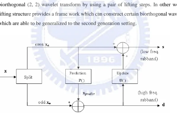
(23) the idea of DPCM (differential pulse code modulation), we record the difference or detail d: d x o P(x e ) .. (2.1). This is because that we expect d is a sparse set, and the first entropy of d is smaller than xo’ s. The operation that calculates a prediction and records the detail is called a lifting step. Some of the spatial correlation is exploited by the prediction steps, but we also need to get some separation in the frequency domain. Frequency separation could be done by applying another lifting step which uses an update operator U on the details to determine a smoothed values s and use it to replace xe: s x e U (d).. (2.2). It is trivial that xe and xo can be reconstructed by applying Eqs. (2.3) and (2.4): xˆ U (d), e s . (2.3). xˆ o d P ( x e ),. (2.4). ˆ where xˆ e and x o are the reconstruction versions of xe and xo, respectively. Hence, the scheme is always invertible and leads to critically sampled perfect reconstruction filter banks. Figure 2.1 shows the block diagram of a pair of lifting steps which contain a prediction and an update lifting steps. According to Figure 2.1, the following Eqs.: x predict (2k 1) P( x(2k ), x(2k 2)) 12 [ x(2k ) x(2k 2)], d (k ) x(2k 1) x predict (2k 1),. U (d (k 1), d (k )) 14 [d (k 1) d (k )],. 9. (2.5a) (2.5b) (2.6a).

(24) s (k ) x(2k ) U (d (k ), d (k 1)),. (2.6b). show a simple example of 5/3 lifting DWT, where Eqs. (2.5a) and (2.6a) are the prediction and update functions, respectively. The xpredict(2k+1) is the prediction value of the odd sample x(2k+1), and it is the average of two nearest even neighbors x(2k) and x(2k+1). The update-function output for an even sample (say x(2k) is a quarter of the detail signal sum of its two odd neighbors (i.e. d(k-1) + d(k+1)). Because of downsampling, d(k) and d(k-1) are corresponded to the original x(2k+1) and x(2k-1), respectively. The reason to use Eq. (2.6a) as the update function is to keep the running average the same as the original x. In wavelet transform Eqs. (2.3)-(2.6) are corresponded to the biorthogonal (2, 2) wavelet transform [18]. Thus, this example implements the biorthogonal (2, 2) wavelet transform by using a pair of lifting steps. In other words, lifting structure provides a frame work which can construct certain biorthogonal wavelets which are able to be generalized to the second generation setting.. Figure 2.1 Block diagram of a pair of lifting steps (prediction and update steps). The x means the input signal vector, and s and d are the output subsampled smooth (low-pass) and detail (high-pass) signal vectors, respectively.. 10.

(25) Representing the wavelet transform in the polyphase form, statements concerning perfect reconstruction can be made by using matrices with polynomial or Laurent polynomial entries. A lifting step is equivalent to an elementary matrix that is a triangular matrix with all diagonal entries equal to one, in matrix algebra. By the theorem in Matrix algebra, any matrix with polynomial entries and determinant one is able to be factored into elementary matrices. From above discussion, we can conclude that every FIR (finite impulse response) wavelet or filter bank can be decomposed into lifting steps.. 2.1.1 Filters and Laurent polynomials Strictly speaking, a (digital) filter [19] suggests a system which passes certain frequency components and totally rejects all others, but in a broader context any system which modifies certain frequencies corresponding to others is also called a filter. A filter is also a linear time-invariant operator which can be completely determined by its impulse response: {h(k ) | h(k ) R, k Z} . Based on the lengths of digital filters, digital filters are commonly classified into two categories which are finite-impulse-response (FIR) and infinite-impulse-response (IIR). The former (FIR) has finite number of non-zero filter coefficients, and the later (IIR) has infinite number of non-zero coefficients. Only FIR filters are discussed in the dissertation. For a linear time-invariant system, the relation among input x, system impulse response h, and the output y is Eq. (2.7): . y (n) x(k )  h(n k ) .. (2.7). k . The most important advantage of IIR filters is that a variety of frequency-selective filters are able to designed using closed-form design formulas. Thus, once the design problem has been specified in terms appropriate for a given approximation method, then the order of the filter which will meet the specifications can be obtained by substitution into some design equations straightforwardly. This advantage makes it feasible to design an IIR filter by manual computation if necessary and it leads to straightforward 11.

(26) non-iterative computer programs for IIR filter design. On the contrarily, FIR filters can have precisely linear phase, although the closed-form design equations do not exist for FIR filters. A Laurent polynomial [20] with coefficients in the field F is an algebraic object typically expressed as that in Eq. (2.8),.  a n z n a( n1) z ( n1)  a0 a1 z a 2 z 2  a n z t  ,. (2.8). where the coefficients ai’ s are elements of F and the number of nonzero terms is finite. For example, the collection of Laurent polynomials with coefficients in a field R form a ring, denoted R[z, z-1], with ring operations given by componentwise addition and multiplication according to Eqs. (2.9) and (2.10), respectively:    a (k )  z k  b( k )  z k [(a (k ) b(k )]  zk ,    k  k  k. (2.9).   k     a (k )  z k  b(k )  z k  a ( i ) b ( j )        z . i , j:i j k k k  k  . (2.10). The equation (2.11): ku. h( z ) h(k )  z k ,. (2.11). k k l. shows the z-transform of a FIR filter h(z), where kl and ku are the smallest and largest k, respectively, for which h(k) is not zero. Thus, Eq. (2.11) is a Laurent polynomial. The degree of a Laurent polynomial h(z) in Eq. (2.11) is defined as Eq. (2.12): | h( z ) |k u k l .. 12. (2.12).

(27) Hence, the length of a FIR filter is the degree of its corresponding Laurent polynomial plus one. By the above definition, zn has degree zero when it is seen as a Laurent polynomial, but it has degree n when it is seen as a regular polynomial. Assume that a(z) and b(z) are two Laurent polynomials with b(z)≠0a nd| a(z)| ≧ |b(z)|. Thus, there always exists two Laurent polynomials q(z) and r(z) with |q(z)| = |a(z)| - |b(z)|, such that a(z) = b(z)q(z) + r(z). The Laurent polynomials q(z) and r(z) are the quotient and remainder respectively of the result that a(z) is divided by b(z), and they are denoted as : q ( z ) a ( z ) / b( z ) ,. and r(z) = a(z) mod b(z). If b(z) is a monomial, then |b(z)| = 0, r(z) = 0, and the division is exact. Any Laurent polynomial is invertible if and only if it is a monomial. Note that for regular polynomials, only constant polynomials are invertible. Another important property is that the long division of Laurent polynomials is not unique. Example 2.1 Assuming a ( z ) z 1 6 z , b( z ) 3 3 z , we want to determine the quotients q(z) and remainders r(z) of that a(z) is divided by b(z). Since the degrees of a(z) and b(z) are 2 and 1 respectively, the quotient q(z) is a Laurent polynomial of degree one. The corresponding remainder can be determined by the relation: r(z) = a(z) –b(z)q(z), and b(z)q(z) has to match a(z) in two terms. 1 If we choose b(z) to match a(z) with z-1 + 6, then q ( z )  ( z 1 5) and r ( z ) 4 z . 3. The degree of the Laurent polynomial r (z) is zero. However, if we let the two match terms. 13.

(28) 1 be z-1 + z, the new answer is q ( z )  ( z 1 1) and r ( z ) 4 . Finally, if we select to match 3 1 6 + z in a(z), then the third answer is q ( z )  (5 z 1 1) and r ( z ) 4 z 1 . 3. From the results of Example 2.1, we see the fact that the division of two Laurent polynomials is not unique, and b(z) has to match a(z) at least |a(z)| - |b(z)| +1 terms. Each selection of q(z) corresponds to a long division algorithm, and this will turn out to be useful later.. 2.1.2 Discrete wavelet transform in FIR form The one-dimensional discrete wavelet transform can be represented as Figure 2.2.. ~ h and g~ are the low-pass and high-pass analysis filters, respectively, and h and g are the low-pass and high-pass synthesis filters, respectively. The blocks (circles) after analysis filters are subsampling units, and the blocks (circles) before synthesis filters are upsampling units. In the dissertation, all the filters in DWT are FIR filters. Equations (2.13) and (2.14) are the requirements for perfect reconstruction: ~ h( z )h ( z 1 ) g ( z ) g~ ( z 1 ) 2,. (2.13). ~ h( z )h (z 1 ) g ( z ) g~ (z 1 ) 0.. (2.14). 14.

(29) DWT. ~ h ( z 1 ) x. IDWT. 2. Low-pass. 2. signal. filter pairs. downsampling. g~ ( z 1 ). 2. h(z ). xˆ. upsampling filter pairs. High-pass signal. 2. g (z ). Figure 2.2 Block diagram of one-dimensional DWT. x is the original signal and xˆis the reconstruction signal of x.. ~ The modulation matrix M(z) and dual modulation matrix M ( z ) are defined in Eqs.. (2.15) and (2.16), respectively: h( z ) h(z )   M ( z )  , g ( z ) g (z )  . (2.15). ~ ~  h ( z ) h (z )  ~ M ( z )  ~ ( z ) g~ (z ). g  . (2.16). Hence, the perfect reconstruction conditions can be represented as ~ M ( z 1 ) t M ( z ) 2 I ,. (2.17). ~ ~ where I is the 2-by-2 identity matrix and M t is the transpose of M . Since all the filters. here are FIR, the modulation and dual modulation matrices belong to GL(2, R[z, z-1]) which denotes a ring whose elements are 2-by-2 matrices with Laurent-polynomial entries, and any matrix from this set is invertible and unitary.. 15.

(30) The polyphase representation of a filter h is given by h( z ) he ( z 2 ) z 1ho ( z 2 ),. where he and ho contains the even and odd coefficient terms of h, respectively. He and ho can be represented as the form in Eqs. (2.18) or (2.19):  he ( z ) h(2k ) z k ,  k  h ( z ) h(2k 1) z k ,   o  k . (2.18). h( z ) h(z )  2 he ( z )  ,  2  h( z ) h(z ) ho ( z 2 )  .  2 z 1. (2.19). and. We define the polyphase matrix as. h ( z ) g e ( z)  P( z ) e , ho ( z ) g o ( z )  . (2.20). 1 z   P( z 2 ) t 12 M ( z )  . 1 z   . (2.21). and then. Similarly, the dual polyphase matrix can be defined as that in Eq. (2.22): ~  he ( z ) g~e ( z )  ~ P ( z )  ~ ~ ( z ). h ( z ) g o o . 16. (2.22).

(31) ~ By using P ( z ) and P(z), the DWT can be represented as shown in Figure 2.3, and the. perfect reconstruction condition is represented as ~ P ( z ) P ( z 1 ) t I .. (2.23). In the Figure 2.3, for DWT side, first, the original signal x is subsampled into even and odd samples, then the susampled results are applied the dual polyphase matrix. For the inverse transform, the transformed inputs are applied the polyphase matrix first, and then the even and odd results are joined to form the reconstruction signal xˆ.. Forward transform. Ieverse transform Lowpass. 2 x. ~ P ( z 1 ) t. z. 2. 2. signal. . P (z ). Highpass signal. subsampling. 2. xˆ. z-1. upsampling. Figure 2.3 The polyphase representation of DWT and IDWT.. ~ Because P ( z ) and P(z) contain only Laurent polynomials, Eq. (2.23) implies that. the determinant and inverse matrix of P(z) are all Laurent polynomials , and that is possible only when det(P(z)) is a monomial (i.e. det(P(z)) = czn, where c R and n Z ). ~ Thus P ( z ) and P(z) are elements in GL(2, R[z, z-1]). If det(P(z)) is not equal to one, then we can divide ge(z) and go(z) by det(P(z)), and then det(P(z)) becomes one. This means that for a specific (given) filter h, the determinant of a polyphase can always be one by 17.

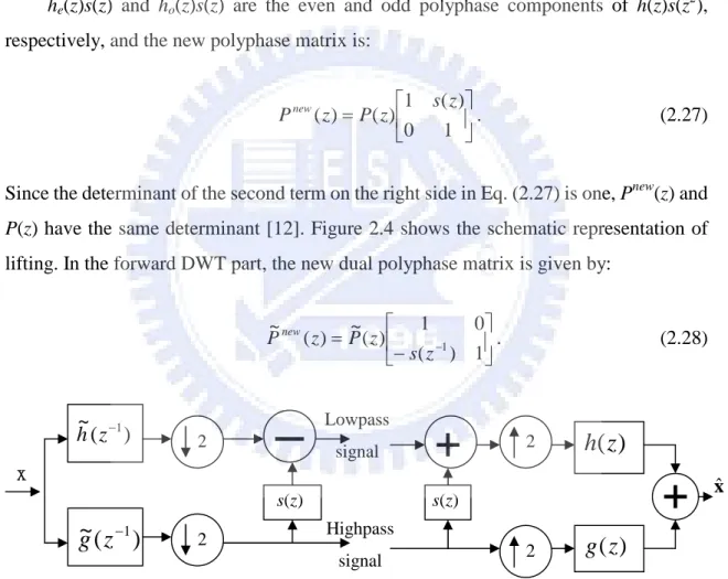
(32) scaling and shifting the filter g. Without loss of generality we assume that det(P(z)) = 1 and P (z )  SL[2; R[z, z-1]]. The problem to find a FIR wavelet transform is equivalent to ~ find a polyphase matrix P(z) with det(P(z)) = 1. For a given P ( z ) and the four filters for. the DWT follow immediately. Solving Eq. (2.23) we have ~ he ( z ) g o ( z 1 ), ~  1 ho ( z ) g e ( z ), ~  1 g e ( z ) ho ( z ), g~ ( z ) h ( z 1 ). e  o. (2.24). g~ ( z ) z 1 h(z 1 ), ~ h ( z ) z 1 g (z 1 ). . (2.25). Equation (2.24) implies. ~ For the simple example P(z) = I, we have h( z ) h ( z ) 1 and g ( z ) g~ ( z ) z 1 . The. DWT only splits the input signal into even and odd samples and downsamples these samples. Such a DWT is named as the Lazy wavelet transform [14] or polyphase transform.. 2.1.3 The lifting structure In DWT, the lifting structure [12]-[14] is a special relationship between perfect reconstruction filter pairs (h, g) which have the same low-pass or high-pass filters. We can begin from the Lazy wavelet and apply lifting to build our way, step by step, up to a multiresolution analysis with particular features. If the corresponding polyphase matrix P(z) of a filter pair (h, g) has determinant one, then the filter pair is complementary. For a complementary filter pair (h, g), its dual filter ~ pair (h , g~ ) is also complementary. Assume that a filter pair (h, g) is complementary.. 18.

(33) Then any other FIR filter, which is denoted as gnew, complementary to h is of the form in Eq. (2.26): g new ( z ) g ( z ) h( z ) s ( z 2 ) ,. (2.26). where s(z) is a Laurent polynomial. In other words, any filter of the form in Eq. (2.26) is complementary to h. he(z)s(z) and ho(z)s(z) are the even and odd polyphase components of h(z)s(z2), respectively, and the new polyphase matrix is: 1 s ( z )  P new ( z ) P( z )  . 0 1   . (2.27). Since the determinant of the second term on the right side in Eq. (2.27) is one, Pnew(z) and P(z) have the same determinant [12]. Figure 2.4 shows the schematic representation of lifting. In the forward DWT part, the new dual polyphase matrix is given by: 0 ~ ~  1 P new ( z ) P ( z )  .  1 s ( z ) 1  . ~ h ( z 1 ). (2.28). Lowpass 2. 2. signal. h(z ). x s(z). g~ ( z 1 ). 2. xˆ. s(z) Highpass signal. 2. g (z ). Figure 2.4 The lifting structure: A classical subband filter scheme followed by a lifting scheme which lifts the low-pass subband with the help of the high-pass subband.. 19.

(34) ~ A new low-pass filter h is given by Eq. (2.29): ~ ~ h new ( z ) h ( z ) g~ ( z ) s ( z 2 ) .. (2.29). Similarly, if (h, g) is complementary, then any other FIR filter hneo complementary to g is of the form: h new ( z ) h( z ) g ( z )t ( z 2 ) ,. (2.30). where t(z) is a Laurent polynomial. Conversely speaking, any filter of this form in Eq. (2.30) is complementary to g. For dual lifting, the new polyphase matrix is 1 0 P new ( z ) P( z )  . t ( z ) 1  . (2.31). Dual lifting generates a new g~ which is: ~ g~ new ( z ) g~ ( z ) h ( z )t ( z 2 ) .. (2.32). The dual lifting structure is shown in Figure 2.5. Sweldens had proposed a family of lifting wavelets which starts from the Lazy wavelet followed by one dual lifting and one primal lifting step. Every h filter constructed this way is half band, and the corresponding scaling function is interpolating.. 20.

(35) ~ h ( z 1 ). Lowpass 2. x. t(z). g~ ( z 1 ). 2. signal. xˆ. t(z) Highpass. 2. h(z ). signal. 2. g (z ). Figure 2.5 The dual lifting structure: A classical subband filter scheme followed by a lifting scheme which lifts the high-pass subband with the help of the low-pass subband.. 2.1.4 The Euclidean algorithm In this section, the Euclidean algorithm is extended to find the greatest common divisor (gcd) of two polynomials, and it will be used to determine the common factors of two Laurent polynomials later [20]. As we have discussed in Example 2.1, the gcd of polynomials is not unique. Actually, the gcd of two Laurent polynomials is defined up to a factor zn (Note that, the gcd of two regular polynomials is up to a constant.). If the gcd of two Laurent polynomials is of degree zero, then the two Laurent polynomials are relatively prime. Euclidean algorithm for Laurent polynomials: Assume there are two Laurent polynomials a(z) and b(z) with |a(z)| ≧ |b(z)| and b(z)≠0.Se ta 0 ( z ) a ( z ) and b 0 ( z ) b( z ) and iterate the following steps beginning from n = 0. a n1 ( z ) b n ( z ),. (2.33). bn+1(z) = an(z) mod bn(z),. (2.34). where the superscripts of Laurent polynomials a(z) and b(z) denote the iteration number. For the smallest n = m that bm(z) = 0, we have am(z) = gcd(a(z), b(z)). Given that 21.

(36) b n 1 ( z ) b n ( z ) , there is an k such that b k ( z ) 0 . The algorithm stops for m = k + 1.. The number of steps is bounded by m (m ≦ |b(z)| + 1). Let qn+1(z) = an(z)/bn(z), then we have.  0 1  a ( z )  a m ( z ) 1          n  1 q ( z ) b( z ) . 0      nm  . (2.35). a ( z ) m    q n ( z ) 1 a m ( z )       ,   b( z )  1 0 0  1 n        . (2.36). Therefore. and am(z) divides both a(z) and b(z). If am(z) is a monomial, then a(z) and b(z) are relatively prime. Example 2.2 Assume that a( z ) a 0 ( z ) z 1 6 z , b( z ) b 0 ( z ) 3 3 z . The first division gives us a 1 ( z ) 3 3z , b 1 ( z ) 4,. and. q 1 13 ( z 1 1). The second iteration gives: a 2 ( z ) 4, b 2 ( z ) 0,. 22.

(37) and. q 2 34 (1 z ). Hence, a(z) and b(z) are relative prime and we have: 1 3 1 4  1  z 1 6 z   1) 1  4 (1 z ) 3 (z .     1   0 0 0     3 3Z   1. It takes 2 (i.e. m = |b(z)| + 1) steps (iterations) to complete the process.. 2.1.5 The factoring algorithm In this section, we will discuss how to factor a pair of complementary filters (h, g) into lifting steps. Note that he(z) and ho(z) must be relatively prime, since any common factor would also divide det(P(z)) and det(P(z)) = 1 is already known. Use the Euclidean algorithm to find the monomial gcd of he(z) and ho(z). Because of the non-uniqueness of the Laurent-polynomial division, we can only select the quotients such that the gcd is a constant. Assume the constant is c, we have that. he ( z )  m  c  q n ( z ) 1   .     ho ( z ) n1  1 0 0   . (2.37). If m is odd, we can multiply h(z) with z and g(z) with z-1. This does not change the determinant of the polyphase matrix, and it flips the polyphase components of h(z) and makes m even. Thus, we can always assume that m is even. Given a filter h(z) we can always find a complementary filter, that is denoted as gcpl, by letting:.  c 0  h ( z ) g ecpl ( z ) m  q n ( z ) 1  P cpl ( z ) e  .     cpl 0 1 / c ho ( z ) g o ( z ) n1  1 0   . 23. (2.38).

(38) Rewrite the second equation in Eq. (2.38) and we have. 0 1  q n ( z ) 1  1 q n ( z )   ,      1 0 0  0 1    1. (2.39). 0 1 0  q n ( z ) 1  1 .     n 1 0 q ( z ) 1 0    1. (2.40). and. When n is odd, use Eq. (2.39), and use Eq. (2.40) for n is even. Thus Eq. (2.38) becomes m/2 c 0  0  1 q 2 n1 ( z ) 1  P cpl ( z )  .     2n q ( z ) 1 0 1 / c 0 1  n 1    . (2.41). At last, the original filter g can be recovered by Eq. (2.26). The filter g can always be recovered from gcpl with one lifting or: 1 s( z )  P( z ) P cpl ( z )  . 0 1   . (2.42). To sum up, if the complementary filter pair (h, g) is given, then there always exist Laurent polynomials sn(z) and tn(z) for 1 n k and a nonzero constant c such that. 0 c 0   1  1 s n ( z ) P( z )  .     n t ( z ) 1 0 1 / c 0 1  n 1     k. 24. (2.43).

(39) 1/c Lowpass signal. 2. x. t1(z). tk(z). 1. s (z). z. k. s (z). c. 2. Highpass signal. Figure 2.6 The forward DWT using lifting structure.. Equation (2.43) means that every FIR filter DWT can be obtained by beginning with the Lazy wavelet followed by k lifting and dual lifting steps followed with a scaling. Similarly, the dual polyphase matrix is given by k 0 1 / c 0  1 t n ( z 1 )  1  ~ P ( z )  n 1     . 0 s ( z ) 1 c 0 1 1  n    . (2.44). Figures 2.6 and 2.7 show the different steps of DWT and IDWT, respectively.. Lowpass. c. 2. signal. Reconstruction. tk(z) Highpass. t1(z). sk(z). 1/c. signal. s1(z). xˆ 2. signal. Figure 2.7 The Inverse DWT using lifting structure.. 25. z-1.

(40) 2.2 Realization of Lifting-Based Discrete Wavelet Transform In this section, the famous Haar wavelet, 5/3 wavelet, and 9-7 wavelet and their corresponding lifting-based realizations are discussed in the following subsections.. 2.2.1 Haar wavelets For the Haar wavelets, we have that h( z ) 1 z 1 , g ( z ) 12 12 z 1 ,. ~ h ( z ) 12 12 z 1 , and g~ ( z ) 1 z 1 . By using the Euclidean algorithm the polyphase matrix can be represented as: 1 1 / 2  1 0 1 1 / 2   P (z )  .     1 1/ 2   1 1 0 1     Therefore, on the analysis side we have: 1 1 / 2 1 0  ~ P ( z ) 1 P ( z 1 )  .  1 1  1 1     Hence, we have the following realization of the forward DWT:  s ( 0) (n) x(2n),  (0)  d (n) x(2n 1),  (0) (0) d (n) d (n) s (n), (0) 1  s (n) s (n) 2 d (n), and the IDWT is given by: s ( 0) (n) s (n) 12 d (n),  (0) (0) d (n) d (n) s (n),  (2n 1) d ( 0) (n), xˆ xˆ (0) (2n) s (n). 26.

(41) In the reverse transform, we use xˆto denote the reconstruction version of x. These signals are shown in Figs. 2.8 and 2.9.. s(0) (n). s (n). 2. Lowpass signal. Input signal. 1/2 d (n) Highpass. z. 2. d(0) (n). signal. Figure 2.8 DWT with lifting Haar wavelet.. Lowpass. s(n). xˆ ( 2n). s(0)(n). 2. signal. Reconstruction signal xˆ. 1/2 Highpass. d(n). d(0)(n). signal. 2. Figure 2.9 IDWT with lifting Haar wavelet.. 27. z-1. xˆ (2n 1).

(42) 2.2.2 The 5/3 wavelets In this section, we will discuss the 5/3 wavelets which was recommended by the new image compression standard JPEG2000. For the 5/3 wavelets, we have that ~ h ( z ) 18 z 2 14 z 1 34 14 z 1 18 z 2 , g~ ( z )   12 z 2  z 1  12 . According to Eqs. (2.18) and (2.19) we have: ~ he ( z 2 ) 18 z 2 34 18 z 2 , ~ 2 ho ( z ) 14 14 z 2 , ~ 2 2 1 1 g e ( z ) 2 z 2 , g~ ( z 2 ) 1. o The dual polyphase matrix of this filter bank is: ~  18 z 2 34 18 z 2 he ( z ) g~e ( z )   ~ P ( z )   ~ 2 ho ( z ) g~o ( z )  14 14 z . 12 z 2 12  . 1 . Assuming perfection reconstruction and complementary filters, the corresponding synthesis filters are: h( z ) z 1 g~ (z 1 ) 12 z 1 1 12 z1 ,. and ~ g ( z ) z 1 h (z 1 ) 18 z 3 14 z 2 34 z 1 14 18 z.. Using the Euclidean algorithm we can factor the dual polyphase matrix as: 1 (1 z ) / 4 1 0   ~ P ( z )  .    1 (1 z ) / 2 1 0 1     Hence, we have the following realization of the forward DWT: 28.

(43) s ( 0 ) (n) x(2n),  (0) d (n) x(2n 1),   d (n) d ( 0 ) (n) 12 [ s ( 0 ) (n) s ( 0 ) (n 1)],  s (n) s ( 0 ) (n) 1 [d (n) d (n 1)], 4 . and the IDWT is given by: s ( 0 ) (n) s (n) 14 [d (n) d (n 1)],  (0) d (n) d (n) 12 [ s ( 0 ) (n) s ( 0 ) (n 1)],   (0) x(2n 1) d (n), x(2n) s ( 0 ) (n). . 2.2.3 The 9/7 wavelets The 9/7 wavelet [22] filter bank was also proposed in Part I of JPEG2000 standard. ~ For the 9/7 filter pair, the analysis filter h has 9 coefficients, and the synthesis filter h has 7 coefficients. Each of the two high-pass filters g~ and g has 4 vanishing moments. For a smoother scaling function, the filter with 7 coefficients is choused to be the synthesis filter. Using the Euclidean algorithm, the most efficient factorization of the dual polyphase matrix of 9/7 wavelets is as follows: 0   1 a(1 z 1 ) 1 c(1 z 1 )  1 ~ P ( z )      b(1 z ) 1 0 1 0 1       K 0 0   1  ,     d (1 z ) 1   0 1 / K . where a = -1.586134342, b = -0.05298011854, c = 0.8829110762, d = 0.4435068522, and K = 1.149604398. Both 5/3 and 9/7 wavelet filters can be represented by banded matrix operations. For the 5/3 wavelet: 29.

(44) Y5 / 3 XM 1 M 2 , where 1   0   0   M 1        . a 0 1 0 0 a 1 a 0 0 1 0 a 0. 1   0   0   M 2        . 0 1 0 0. 0 0 1 0 0. 0 a 0 1 0 0 a 1 a 0 0 1 0 a.        ,   0  0 1 . and 0 b 0 1 0 0 b 1 b 0 0 1 0 b 0. 0 0 1 0 0. 0 b 0 1 0 b 1 0 0. The IDWT can be represented as 1. 1. X Y5 / 3 M 2 M 1 . For the 9/7 wavelet, we have: Y9 / 7 XM 1 M 2 M 3 M 4 ,. 30.        .   0  0 1 .

(45) 1   0   0   M 3        . c 0 1 0 0 c 1 c 0 0 1 0 c 0. 1   0   0   M 4        . 0 1 0 0. 0 0 1 0 0. 0 c 0 1 0 0 c 1 c 0 0 1 0 c.        ,   0  0 1 . and 0 d 0 1 0 0 d 1 d 0 0 1 0 d 0. 0 0 1 0 0. 0 0 0 d 1 0 0 d 1.        .   0  0 1 . Finally, the IDWT based on 9/7 wavelet can be represented as: 1. 1. 1. 1. X Y9 / 7 M 4 M 3 M 2 M 1 .. 2.3 Lifting-Based Direction-Adaptive DWT (DA-DWT) The conventional separable 2-D DWT can be implemented by consecutively applying 1-D DWT in horizontal and vertical directions, or vice versa. That means if we use the lifting structure to implement 2-D DWT, the prediction and update directions are parallel to the horizontal axis or the vertical axis. The lifting-based DWT whose 31.

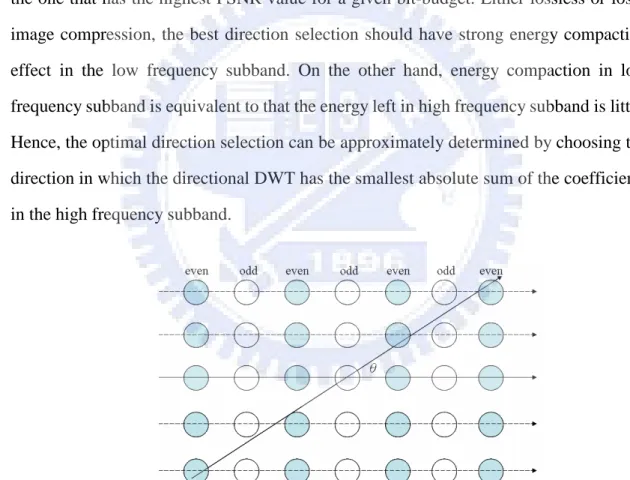
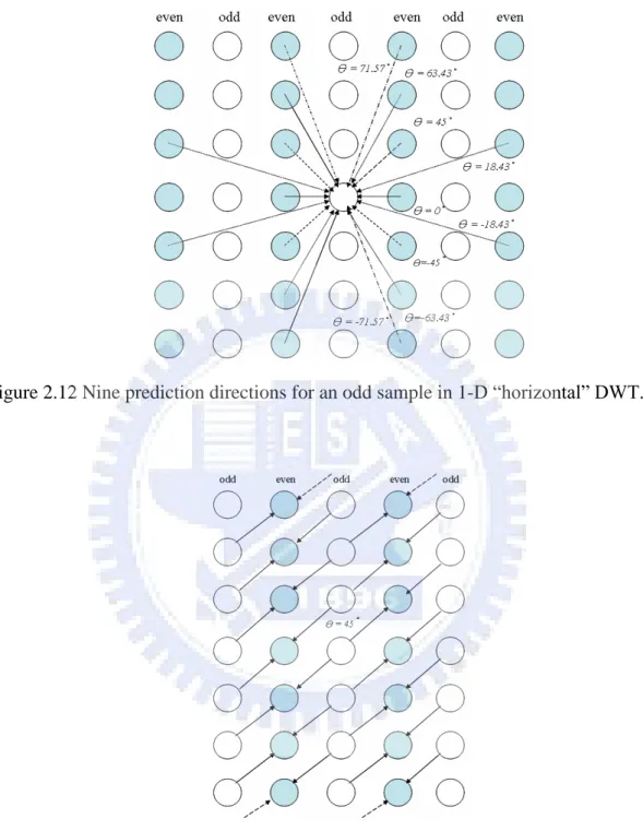
(46) directions of prediction and update steps are adaptive is called a direction-adaptive DWT (DA-DWT) or adaptive directional lifting-based DWT (ADL-DWT). The DA-DWT can be decomposed into two blocks which are shown in Figure 2.10. First, an input image is partitioned into many small blocks and the best transform direction for each block is determined. Then, lifting DWT is performed on the image according to the partition and direction information obtained in the first block. Figure 2.11 shows the direction of the lifting step of a direction-adaptive DWT, and the prediction and update direction line intersects the horizontal axis by an angle θ . Applying the sub-pel technique, although the angle θc a nbea nyva l uebe t we e n0a ndπ/ 2( r a di a ns )i n[ 3], only nine directions were used. In [4], they also used nine directions for prediction and update, but these nine directions were different from those in [3]. In this dissertation, we use the directions in [4], because this method does not involve complex sub-pel computation and has better performance. Figure 2.11 shows the nine directions and their corresponding neighbors of an odd sample in prediction step of a 5/3-wavelet DWT. In Figure 2.13, each of the even samples is updated by its two odd neighbors along the line with θ= 45 degrees.. Input image. Transformed. Partition &. Lifting DWT. Direction selection. image. Figure 2.10 The block diagram of a DA-DWT system.. ADL-DWT [3] and DA-DWT [4] are proposed to compress a rectangular image by dividing the whole image into a lot of fixed-size small square blocks. After dividing an image into many small square blocks, the optimal direction for directional lifting DWT of each block is determined. Then, some connected blocks with the same lifting direction are 32.

(47) grouped to form a large rectangular block with the same direction for saving the bits of side information [4]. Different from the method in [4], the method used in [3] splits a larger square block into several small rectangular blocks instead of merging some small square blocks to form a larger rectangular block. For lossless image compression, the best direction (θ) of prediction and update of the directional lifting DWT is the direction that spends the least amount of bits to compress this (square or rectangular) block. For lossy image compression, the best direction of the directional lifting DWT in a block should be the one that has the highest PSNR value for a given bit-budget. Either lossless or lossy image compression, the best direction selection should have strong energy compaction effect in the low frequency subband. On the other hand, energy compaction in low frequency subband is equivalent to that the energy left in high frequency subband is little. Hence, the optimal direction selection can be approximately determined by choosing the direction in which the directional DWT has the smallest absolute sum of the coefficients in the high frequency subband.. Figure 2.11 A Direction selection example with angle θin 1-D“ hor i z ont a l ”DWT.. 33.

(48) Figure 2.12 Nine prediction directions for an odd sample in 1-D“ hor i z ont a l ”DWT.. Figure 2.13 The update stage with θ= 45o.. The last step of the 1-D directional DWT is a subsampling stage, and the subsampling method is just like the way in the conventional DWT, i.e. the subsampling 34.

(49) di r e c t i oni st hehor i z ont a ldi r e c t i onf ora“ r ow”directional adaptive DWT. After the “ r ow”di r e c t i ona la da pt i veDWTi sc ompl e t e ,t he“ c ol umn”di r e c t i onDWTi spe r f or me d on the whole segment block, and the last step is the subsampling step following the “ c ol umn”di r e c t i ona l DWTi naone -level direction-adaptive DWT. The realization of the “ c ol umn”di r e c t i on-a da pt i veDWTi st hes a mea st he“ r ow”di r e c t i on-adaptive DWT, if t hes e g me ntbl oc ka f t e r“ r ow”di r e c t i on-adaptive DWT is rotated clockwise 90 degrees.. 2.4 Shape-Adaptive DWT (SA-DWT) Because of fast growth of multimedia applications, the needs of searching, accessing, indexing, and manipulating visual information at the semantically meaningful object level are becoming more and more urgent. The MPEG-4 standard supports such a functionality of making a visual object available in the compressed form, and this functionality provides flexibility for manipulating a visual object in multimedia applications and improves the compression efficiency in very low bit-rate coding. There are two major parts in an object-based video coding system. One is the intra frame coding, and the other is the inter frame coding. The inter frame coding involving motion prediction, which will not be discussed here, and we focus on the intra frame coding in this subsection. The intra frame coding of the object-based video coding can be divided into object shape coding and object texture coding. The alpha map (Figure 2.14 (b)) is used to represent the region that the object occupied, and the simplest alpha map can be a binary figure which has value 1 for the bits in the object and value 0 for each bit outside the object. Thus, using the alpha map, the object in an image can be easily segmented. The most popular technique for object texture coding is the shape-adaptive DCT (SA-DCT) [23], which uses 8-by-8 blocks to represent the object to be transformed and coded. Since an object usually can not be covered by 8-by-8 blocks perfectly, a lot of boundary blocks do not totally reside in the object and make this method inefficient. S. Li et al. proposed a shape-adaptive discrete wavelet transform (SA-DWT) for arbitrarily shaped visual object coding [1], and they used the SA-DWT for the texture coding of the intra frame part in object based video coding. Lu et al. also proposed an object texture coding technique [2] 35.

(50) that combined a SA-DWT and the SPECK algorithm. The experimental results in [1] showed that the SA-DWT with extentions of zerotree entropy coding (ZTE) outperforms SA-DCT up to 0.97 dB in Y-plane PSNR, 1.29 dB in U-plane PSNR, and 0.89 dB in V-plane PSNR, for the Akiyo sequence (CIF) at 1.0 bpp. However, the SA-DWTs using conventional DWTs have the disadvantage that they need complicated rules to handle the even and odd problems of the samples. In Chapter 4, the lifting DWTs are introduced to realize the shape-adaptive functionality that we call lifting-based shape-adaptive DWT (LSA-DWT).. Figure 2.14 The original image and alpha map of object 1: (a) the test visual object 1 with background (256-by-256), (b) the shape mask (alpha map).. 36.

(51) CHAPTER 3 TWO WAVELET-BASED HYBRID CODECS FOR IMAGE COMPRESSION In this chapter, two image compression applications of DWT will be discussed. Both of them are wavelet-based applications, so the lifting-based DWT can seamlessly replace the conventional DWTs in these two applications. The first one, in Section 3.1, proposed a hybrid image coder which combines SPIHT (set partitioning in hierarchical trees) [24], DWT, and vector quantization [25][26] for improving image compression efficiency. In Section 3.2, the second application used DWT, SPECK (set-partitioning embedded block coder) [27], and residual vector quantization (RVQ) to enhance image compression performance.. 3.1 Image Compression Using SPIHT and VQ Su et al. presents a hybrid coding system using a combination of set partition in hierarchical trees (SPIHT) and vector quantization (VQ) for image compression [28]. In which, the wavelet coefficients of the input image are rearranged to form the wavelet trees that are composed of the corresponding wavelet coefficients from all the subbands of the same orientation; a simple tree classifier has been proposed to group these wavelet trees into two classes based on the amplitude distribution; and each class of trees is to be coded using an appropriate procedure, specifically either SPIHT or VQ. Experimental results show that advantages gained by combining the superior coding performance of VQ and efficient cross-subband prediction of SPIHT are, as expected, appreciable for the compression task, especially for many natural images with large portions of textures.. 37.

(52) 3.1.1 Overview of SPIHT The SPIHT algorithm has received a lot of attention since its introduction for image compression in 1996. It contains two passes: sorting pass and refinement pass, which can be combined to form a single scan pass. Three symbols: zero tree (ZT), insignificant pixel (IP) and significant pixel (SP) are used to code the wavelet tree structure of images, which are stored in their respective lists: list of insignificant sets (LIS), list of insignificant pixels (LIP) and list of significant pixels (LSP). Below is the encoding algorithm presented in four steps [24]. log 2 (max ( m , n ) c m ,n ), where c m ,n is the wavelet tree node at 1) Compute b . coordinate (m, n) . Set the initial threshold T 2 b . 2) Sorting pass: identify the coefficients such that T c m ,n 2T ; output their respective coordinates and signs. 3) Refinement pass: output the b-th (most significant) bit of all the tree nodes with c m ,n 2T following the same order used to output the coordinates in previous. sorting passes. 4) Decrease b by one, halve the threshold T and go to step 2. The scan pass (i.e. Step 2 followed by Step 3) of SPIHT is performed in a recursive manner until the expected bit rate is reached. In sorting pass, the coefficients in LIS and LIP are evaluated as follows. For coefficients whose magnitudes are greater than or equal to the current threshold, they become significant and will be moved to LSP. For insignificant coefficients whose magnitudes are less than the current threshold, they will. 38.

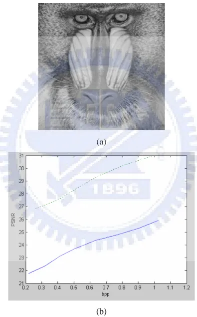
(53) be stored in LIS if all their descendants are also insignificant with respective to the same threshold; or otherwise, stored in LIP. A sequence of successively smaller thresholds can be obtained by using the following recursive equation: Tk 0.5 Tk 1 ,. (3.1). where the initial threshold T1 must be greater than or equal to half the maximum magnitude of the transform coefficients. After the k-th sorting pass, tree nodes whose magnitudes are in the range: [Tk , Tk 1 ) for k 1 (or [T1 , ) for k 1 ) will be stored in LSP with one bit per node to indicate their respective signs. In refinement pass, the significant nodes stored in LSP are refined with one bit per node to update their respective information. The great success of SPIHT is attributed to the important hypothesis of wavelet transform: if a parent node is insignificant, then all its descendants are likely to be insignificant with respect to the same threshold and therefore these insignificant nodes can be efficiently coded with a single symbol ZT.. 3.1.2 Proposed hybrid coding For images with textures composed mainly of the middle and high frequency components, there are many significant nodes whose ancestors are insignificant. It follows that zero trees of insignificant nodes are very rare. Figure 3.1 (a), for example shows a 256×256 grayscale Mandrill image with large portions of high frequency textures. Empirically, we have classified the wavelet trees into two classes based on the magnitude distribution. The compression performance of SPIHT is evaluated for each class of wavelet trees. As shown in Figure 3.1 (b), where the horizontal and vertical axes are the 39.

(54) compression rates measured in bits per pixel (bpp) and peak signal to noise ratio (PSNR) values measured in dB, respectively, the SPIHT algorithm is much more effective for one class of wavelet trees than the other.. (a). (b). Figure 3.1 Rate-distortion curves of the low frequency (dotted line) and high frequency (solid line) wavelet trees of Mandrill image by using the SPIHT algorithm. 40.