稀少和非稀少的潛在類別迴歸模型之適合度檢定

國 立 交 通 大 學

統計學研究所

碩 士 論 文

稀少和非稀少的潛在類別迴歸模型之適合度檢定

Goodness-of-fit Test for Sparse and Unsparse

Latent Class Regression Models

研 究 生 ：鄭俊凱

指導教授 ：黃冠華 博士

稀少和非稀少的潛在類別迴歸模型之適合度檢定

Goodness-of-fit Test for Sparse and Unsparse

Latent Class Regression Models

研 究 生：鄭俊凱

Student ： Chun-Kai Cheng

指導教授：黃冠華

Advisor ： Dr. Guan-Hua Huang

國 立 交 通 大 學

統計學研究所

碩 士 論 文

A Thesis

Submitted to Institute of Statistics

College of Science

National Chiao Tung University

in Partial Fulfillment of the Requirements

for the Degree of

Master

in

Statistics

June 2006

Hsinchu, Taiwan, Republic of China

中華民國九十五年六月

稀少和非稀少的潛在類別迴歸模型之適合度檢定

研究生：鄭俊凱 指導教授：黃冠華 博士

國立交通大學統計學研究所

摘要

潛在類別迴歸( latent class regression ) 模型被廣泛利用在先前的許多文

獻裡，這種模型能將多重指標的共同特徵整合成基本的類別變數。這篇論文

中我們將提出ㄧ個潛在類別迴歸模型的適合度檢定，此檢定的基礎是由所有

可能回答的選項以及相伴變數分群所組成的列聯表，這個概念是由 Hosmer

與 Lemeshow 在邏輯斯迴歸中所提出來的。而當列聯表有稀少情形發生時，

我們將用一階和二階邊際來取代並且修正檢定統計量。我們在不同的條件下

作模擬，來測試所提出的適合度檢定表現。

Goodness-of-fit Test for Sparse and Unsparse

Latent Class Regression Models

Student：Chun-Kai Cheng Advisor：Dr. Guan-Hua Huang

Institute of Statistic

National Chiao Tung University

ABSTRACT

Latent class regression (LCR) models have been utilized previously in

many literatures. Such models can summarize shared features of the multiple

indicators as an underlying categorical variable. In this paper, we propose a

goodness-of-fit for the LCR model. The basis of the proposed test is a

contingency table, which groups the population through all possible response

patterns and concomitant covariates. The idea is from Hosmer-Lemeshow

statistic for the multiple logistic regression model. When the contingency

table is sparse, we replace it with the first- and second-order marginals and

modify the test statistic. A simulation study is carried out to examine the

behavior of the proposed goodness-of-fit test under different situations.

誌謝

在交大統計研究所學習的這兩年，要謝謝所上的各位教授細心教

導，也要感謝自己的指導教授黃冠華老師，不厭其煩的指導來協助我解

決遭遇到的許多難題，讓論文能夠順利的完成。另外也要感謝黃文瀚老

師、徐南蓉老師以及陳鄰安老師，在口試時給予我建議，並指正我論文

裡需要修改的地方。

我也要感謝研究所同學明曄、泓毅、志強、秀慧…等，以及我的女

朋友和我的家人，在各方面給我的幫助和鼓勵，讓我能快樂、順利完成

這兩年學業。最後將此論文獻給我的家人、朋友、統計所同學及學弟妹。

鄭俊凱 謹誌于

國立交通大學統計學研究所

中華民國九十五年六月二十八號

Contents

Abstract (in Chinese) i

Abstract (in English) ii

Acknowledgement (in Chinese) iii

Contents iv

List of tables vi

1 Introduction 1

2 Literature Review 3

2.1 Latent class regression model . . . 3 2.2 Goodness-of-fit test for logistic regression . . . 4 2.3 General chi-squared statistic for individual likelihood and

ran-dom cells . . . 6 2.4 First and second-order marginals . . . 10

3 Methodologies 12

3.1 Goodness-of-fit test of LCR model . . . 12 3.2 First- and second-order marginals of LCR model . . . 15

4 Simulation Studies 18

4.1 Generated data from the LCR model . . . 18 4.2 Assess power of the proposed test statistics . . . 20

Appendix 23

List of Tables

1 Notational set-up of the frequencies in logistic regression model 33

2 Notational set-up of the frequencies in LCR model . . . 33

3 Interpretation of the silhouette coefficient for partitioning method 33 4 Notational set-up of the frequencies of first- and second-order marginals . . . 34

5 Values of α0 and αLm in balanced case . . . 35

6 Values of β0 and βP j in balanced case . . . 35

7 Values of α0 and αLm in unbalanced case . . . 35

8 Values of β0 and βP j in unbalanced case . . . 35

9 Observed contingency table of balanced case, averaging over 100 simulations . . . 36

10 Observed contingency table of unbalanced case, averaging over 100 simulations . . . 37

11 Observed contingency table of first- and second-order mar-ginals, averaging over 100 simulations . . . 39

12 Simulation results of ”situation 1” in balanced case . . . 40

13 Simulation results of ”situation 2” in balanced case . . . 40

14 Simulation results of ”situation 3” in balanced case . . . 41

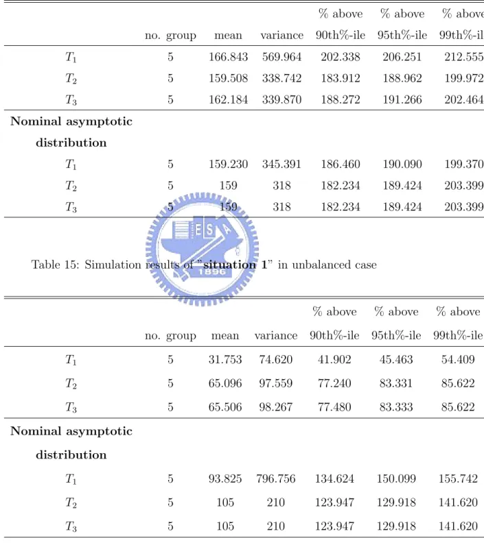
15 Simulation results of ”situation 1” in unbalanced case . . . . 41

16 Simulation results of ”situation 2” in unbalanced case . . . . 42

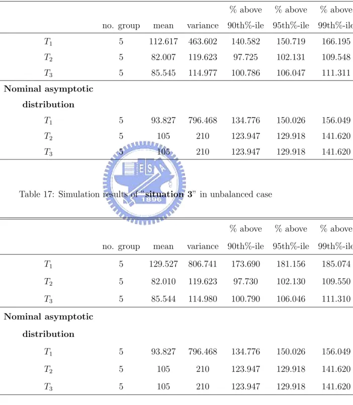
17 Simulation results of ”situation 3” in unbalanced case . . . . 42

18 Power of ”situation 1” in balanced case . . . 43

19 Power of ”situation 2” in balanced case . . . 43

21 Power of ”situation 1” in unbalanced case . . . 44

22 Power of ”situation 2” in unbalanced case . . . 44

1

Introduction

In recent years, questions of psychosocial and medical research investigate the relationship between multiple categorical outcome variables and continu-ous predictor variables. These relationships may be unobserved, hence valid surrogates are necessary. Latent class regression (LCR) models (Huang and Bandeen-Roche 2004) are useful tools for assessing association of measured indicators. The LCR model allow both the distribution of the underlying class variable and the within-class distributions of measured indicators to be functionally related to individual-level independent variables. Hence, LCR model may mitigate errors in measurement and can give well-summarized inference between multiple indicators and covariates of interest. However, we do not observe the true class membership of individuals. So we should carefully do model checking.

When no covariates, the population can be grouped by all possible re-sponse patterns. Pearson χ2 _{test and log likelihood ratio test statistic (LRT)}

(Doodman 1974, Bartholomew 1987, Formann 1992) can be applied for eval-uating overall model fit. However, when there are continuous covariates, Pearson χ2 _{test is invalid because the degree of freedom increases when}

sam-ple size increases.

In this paper, we apply the idea of the Hosmer-Lemeshow statistic (Hos-mer and Lemeshow 1980) to our LCR model. We extend the outcome variable into not only binary but category and each individual has multiple outcome variables. Therefore, an adequate chi-square test statistic can be used to assess to our LCR model. Sometimes, when response patterns are large and

sample size is moderate or small, some cells of the contingency table formed by the all response patterns will be sparse. In this situation, the chi-square test is also not valid. When sparseness occurs, informal remedies such as combining cells are often recommended. Here, we substitute the first-order and second-order marginal frequencies (Reiser and Lin 1999) for the original contingency table, and then we modify the chi-square test statistic which is mentioned above.

In section 2, we review four parts: 1.The LCR model and some assump-tions which complete the model; 2.The goodness-of-fit of the multiple logistic regression model; 3.Theorem5.1 in Moore and Spruill (1975) and its required regularity conditions, which is applied to prove the asymptotic distribution of the proposed goodness-of-fit test; 4.The approach of second-order mar-ginal frequencies. In section 3, we propose the goodness-of-fit of our LCR model and propose another test statistic when sparseness occurs. Section 4 presents the results of a simulation study and power of the test statistic. Some discussions and recommendation are presented in section 5.

2

Literature Review

2.1

Latent class regression model

To describe the latent class regression (LCR) model (Hung and Bandeen-Roche 2004), let Yi = (Yi1,. . . , YiM)T represent the M×1 response vector

for the ith individual in a study sample of N persons. Yim can take value

{1,. . . , Km}, where Km ≥ 2, m = 1,. . . , M . And let (xi, zi) be the

concomi-tant covariates of the ith person, where xi = (1, xi1,. . . , xip)T are primary

predictors for latent class membership Si, Si can take values {1,. . . , J}, and

zi = (zi1,. . . , ziM) with zim = (zim1,. . . , zimL)T, m = 1,. . . , M , are secondary

covariates used for P r(Yim = k|Si = j). These covariates may include any

combination of continuous and discrete measures, and they may be mutually exclusive or overlapped. Then the LCR model can be represented as

P r(Yi1= y1, . . . , YiM = ym|xi, zi) = J X j=1 {ηj(xi) M Y m=1 Km Y k=1 [pmkj(zim)]ymk}. (1)

with ηj(xi) and pmkj(zim) as in the generalized linear framework (McCullagh

and Nelder 1989). Here, ymk = I(ym = k) = 1 if ym = k ; otherwise. Various

link functions could be chosen like probit, ordinal, or etc. We specifically propose to use the generalized logit link function (Agresti 1984) :

log · ηj(xi) ηJ(xi) ¸ = β0j + β1jxi1+ . . . + βpjxip = xTi βj, (2) and log · pmkj0(z_im) pmKmj0(zim) ¸ = γmkj0+ α_1mkz_im1+ . . . + α_Lmkz_imL = γ_mkj0+ zT_imα_mk, (3) for i = 1,. . . , N ;m = 1,. . . , M ;k = 1,. . . , Km− 1;j = 1,. . . , J − 1;j0 = 1,. . . , J.

Parameters, γmkj, αmkand βjcan be estimated by Expectation-Maximization

(EM) algorithm (Dempster, Laird and Rubin 1977). EM algorithm is an it-erative approach which is usually for computing maximum likelihood when model includes missing data.

Adding following three assumptions can complete the model (1) : 1. Latent class membership probabilities are associated with only :

P r(Si = j|xi, zi) = P r(Si = j|xi) = exp(xT i βj) 1 +PJ−1_l=1 exp(xT i βl) , j = 1, . . . , J−1

2. Conditioning on class membership, measured responses are associated with zi : P r(Yi1 = y1, . . . , YiM = ym|Si, xi, zi, ) = P r(Yi1 = y1, . . . , YiM = ym|Si, zi) with P r(YiM = k|Si = j0, zi) = exp(γmkj0 + zT_imα_mk) 1 +PKm−1 s=1 exp(γmsj0+ zTimαms) , f or m = 1, . . . , M; k = 1, . . . , Km− 1; j0 = 1, . . . , J.

3. The multiple measurements are conditionally independent given class membership and zi : P r(Yi1 = y1, . . . , YiM = ym|Si, zi) = M Y m=1 P r(Yim= ym|Si, zi)

2.2

Goodness-of-fit test for logistic regression

Hosmer and Lemeshow (1980) proposed a goodness-of-fit test, which de-termines the adequacy of the fitted multiple logistic regression model. The logistic regression model will be stated as follows :

Let Yi= 0 or 1 be outcome variables and xTi = (xi1,. . . , xip) be the

indepen-dent variables. Let π(xi) = P r(Yi = 1|xi) = exp(β0+ βTxi)/(1 + exp(β0+

βT_x

i)) where βT = (β1, . . . , βp). Under these assumptions, the likelihood

function is : L(y; x, β0, β) = n Y i=1 πyi i (1 − πi)1−yi , where πi = π(xi), f or i = 1, . . . , n.

From log of L(y; x, β0, β), the maximum likelihood estimates ˆβ0 and ˆβ

by solving (p + 1) likelihood equations. The basis of Hosmer-Lemeshow statistic builds on a 2×g contingency table. To obtain the table, let ˆπi =

π(xi)|_(β

0,β)=( ˆβ0,βˆ) and define a random variable W where wi = j if cj−1 ≤

ˆ

πi < cj , for j = 1,. . . , g ; i = 1,. . . , n . The cj0s are known constants such

that 0 = c0 < c1 <. . . < cg−1 < cg = 1 .Denote the counts in the cell of table

as nkj where nkj is the frequency of occurrence of the pair (yi = k, wi = j) in

the sample, k = 0, 1 and j = 1,. . . , g. Notationally the observed frequencies may tabulated as Table 1.

A choice of forming c0,. . . , cg in the 2×g contingency table is to make the

distribution of W to be uniform. That is, the cut points c0,. . . , cg depend

on the data and hence are no longer fixed constants. So there will be n/g value of in each interval. Let’s define ˆπ(1) ≤ ˆπ(2) ≤ . . . ≤ ˆπ(n) as the ordered

values of ˆπ and let ˆcj = ˆπ[jn/g], where

h

jn g

i

represents the largest integer less than or equal to jn_g , j = 0,. . . , g. Let ˆwi = j if ˆcj−1 ≤ ˆπi < ˆcj. Define

ˆ

nkj as the observed frequency of the pair (yi = k, ˆwi = j) in the sample. If

ˆ

Jj = {i : ˆcj−1≤ ˆπi < ˆcj} then the test statistic is

Cg = g X j=1 {(ˆn1j− P r∈ ˆJjπˆr) 2 P r∈ ˆJjπˆr + h ˆ n0j− P r∈ ˆJj(1 − ˆπr) i₂ P r∈ ˆJj(1 − ˆπr) } (4)

There are two problems for the application of the usual theory used for chi-square goodness-of-fit test to the distribution of Cg.

1. Parameter estimates are determined using likelihood functions for ”un-grouped” data.

2. The frequencies, ˆnkj in the 2 × g contingency table depend on the

estimated parameters, namely the cells are random not fixed.

Chernoff and Lehmann (1954) first mention a chi-square test under prob-lem 1 and then Watson (1959). Moore(1971) and Moore and Spruill (1975) considered the distribution of the chi-square goodness of fit statistic under both problems 1 and 2. They extended Watson’s results to the case of random rectangular cells. Drust (1979) generalized these results to include random cells other than rectangles. By results of Moor and Spruill (1975) and Drust (1979), the asymptotic distribution of Cg can be obtained as follows.

Theorem Under distributional assumptions, the distribution of Cg will be

asymptotically (N → ∞) χ2_{(2g − g − (p + 1)) +} p+1 X i=1 λiχ2i(1)

where 0 < λi ≤ 1, i = 1,. . . , (p + 1), and λ0is are eigenvalues of some matrix.

The detailed statement of the matrix can see Theorem 1 in 3.1.

2.3

General chi-squared statistic for individual

likeli-hood and random cells

The proof of the above theorem follows from verifying that the regularity conditions necessary for the proof of theorem 4.2, lemma 5.1 and theorem

5.1 in Moore and Spruill (1975) are satisfied.

Before describing these results, the notations are defined as follows. Let

F (y|θ, η) be the cdf of {Y1,. . . , Yn}. The parameter θ ranges over an open

set Ω1in Rm, while η ranges over a neighborhood of a point η0in Rp. The cells

for the following χ2_{tests are rectangles in R}k_{. They are functions of a variable}

ϕ defined on Ω2 in Rr. The resulting cells are denoted by Iσ(ϕ). Here, the

null hypothesis (H0) is that Yi have a cdf F (y|θ, η0). We will explore the

large-sample behavior of tests for the null hypothesis under the sequences of parameter values (θ0, ηn) where θ0 ∈ Ω1 and ηn = η0+ n−1/2γ for fixed γ in

Rp_{. H}

0 is the special case γ = 0. θ is estimated by θn = θn(Y1,. . . , Yn).

The cells are chosen by ϕn = ϕn(Y1,. . . , Yn). We will assume that under

(θ0, ηn), ϕn− ϕ0 = op(1) for some ϕ0 and θn− θ0 = op(1). We will suppress

arguments θ, ϕ, η whenever they take the values θ0, ϕ0, η0 respectively.

The number of Y1,. . . , YN falling in the cell Iσ(ϕ) will be denoted by

Nnσ(ϕ). The cell probabilities are denoted by pσ(θ, η, ϕ) where σ = 1, 2,. . . , p×

g and pσ(θ, η, ϕ) =

R

Iσ(ϕ)dF (x|θ, η).

The regularity conditions for the following theorem are as :

A1. Under (θ0, ηn), θn− θ0 = Op(n−1/2) and ϕn− ϕ0 = op(1). Every vertex

x(ϕ) of every cell Iσ(ϕ) is a continuous Rk-valued function of ϕ in a

neighborhood of ϕ0.

A2. For each σ, pσ(θ, η, ϕ) is continuous in (θ, η, ϕ) and continuously

differ-entiable in (θ, η) in a neighborhood of (θ0, η0, ϕ0). Moreover,

P_M

1 pσ =

A3. F (x) = F (x|θ0, η0) is continuous at every vertex x(ϕ0) of every cell

Iσ(ϕ0). As n → ∞, supx|F (x|ηn) − F (x)| → 0.

A4. K(θ, ϕ) = S(θ, ϕ)S(θ, ϕ)T _{for an M × M matrix S(θ, ϕ) with entries}

continuous in (θ, ϕ) at (θ0, ϕ0). A5. Under (θ0, ηN) n1/2_(θ n− θ0) = n−1/2 N X i=1 h(Yi, ηn) + Aγ+ op(1)

for some m × p matrix A and measurable function h(x, η) from Rk_{× R}p

to Rm _satisfying

E [h(Y, ηn)|(θ0, ηn)] = 0

E£h(Y, ηn)h(Y, ηn)T|(θ0, ηn)

¤

= L(ηn)

where L(ηn) is a m × m matrix converging to the finite and matrix

L = E£h(Y)h(Y)T¤ _{as n → ∞}

Theorem 4.2 in Moore and Spruill (1975)

Let Vn(θn, ϕn) be a M × 1 vector with σth component

vnσ(θn, ϕn) = Nnσ(ϕn) − npσ(θn, η0, ϕn) [npσ(θn, η0, ϕn)]1/2 Define also, qT _{= (p}12 1,. . . , p 1 2 M)

B is a M × m matrix and has (i, j)th entry p−1/2_i ∂pi

∂θj . J = E£(∂logf_∂θ )(∂logf_∂θ )T¤ P = IM − qqT + BLBT − BE £ h(Y )W (Y )T¤_{− E}£_{W (Y )h(Y )}T¤_BT

P

0 = ST

P

S

If A1,. . ., A5 hold, VT

n (θn, ϕn)k(θn, ϕn)Vn(θn, ϕn) has limiting distribution M X j=1 λjχ21j under (θ0, η0) Where λ0 js are eigenvalues of P 0

One more regularity condition is needed for the following lemma : C1. m ≤ M and the matrix with entries ∂pi/∂θj has rank m.

Lemma 5.1 in Moore and Spruill (1975) When C1 regularity condition holds 1. £PT_qqT_{P e}¤ j = 0 j = 1,. . . , M − 1 £ PT_qqT_{P e}¤ j = 1 j = M 2. £PT_{CP e}¤ j = 0 j = 1,. . . , M − m − 1, M £ PT_{CP e}¤ j = 1 j = M − m,. . . , M − 1 3. £PT_BJ−1_BT_{P e}¤ j = 0 j = 1,. . . , M − m − 1, M £ PT_BJ−1_BT_{P e}¤ j = 1 − λj j = M − m,. . . , M − 1

where P is an orthogonal matrix which simultaneously diagonalizes qqT_{, C}

and BJ−1_BT_{. C = B(B}T_B)−1_BT_.

More regularity conditions are needed for the following theorem :

C2. logf (x|θ, η) is differentiable with respect to (θ, η) at (θ0, η0). The

ma-trix J is pd and J12 is finite. (∂/∂θ)F (x|θ) may be evaluated by

C3. n1/2_(ˆθ

n− θ0) = n−1/2

P_n

i=1J−1 ∂logf (Y∂θi|ηn) + J−1J12γ + op(1). Here J is

the information matrix for F (x|θ) at θ0.

J = E · (∂logf ∂θ )( ∂logf ∂θ ) T ¸ , J12 is the m × p matrix J12 = E · (∂logf ∂θ )( ∂logf ∂η ) T ¸ . C4. J − BT_{B is pd.}

Theorem 5.1 in Moore and Spruill (1975)

When A1,. . ., A5 and C1,. . ., C4 regularity conditions hold, k Vn(ˆθn, ϕn) k2

has limiting distribution

χ2_{M −m−1}+

M −1_X j=M −m

λjχ21j under (θ0, η0)

and λM −m,. . . , λM −1 are the m roots of the determinantal equation

|BTB − (1 − λ)J| = 0

2.4

First and second-order marginals

In practice, when response patterns are large and the sample size, n, is

moderate or small, some response patterns of Y0

is are usually less than 5

even to 0. This kind of contingency table is said to be sparse (Agresti and Yang 1987). However, the chi-square approximation for the test distribution may not be valid. So when sparseness occurs, informal remedies such as combining cells or adding a small constant like 0.5 to each cell are sometimes

recommended. One kind of combining method is first order and second-order marginals (Reiser and Lin 1999). The advantage of it is that the frequencies are almost always substantially larger than zero, even with small samples. The combing technique states as follows :

To make the presentation clear, we assume dichotomous response cases. Let Yi= 0 or 1 be outcome variables, for i = 1,. . . , k. The response patter is

a k-dimensional vector of zeros and 1’s. A set of T response patterns can be generated by varying the index of the kth variable most rapidly, the k − 1th variable next, etc. Let πs(β) represent probability of response pattern s and

wis represent element i of response pattern s. Under the model, the first

order and second-order marginal proportion for variable Yi and Yj can be

defined as Pi(1|β) = P (Yi = 1|β) = X s wisπs(β) , Pij(1, 1|β) = P (Yi = 1, Yj = 1|β) = X s wiswjsπs(β) ,

The summation across the frequencies associated with the response pat-terns to obtain the marginal proportions represents a transformation of the

frequencies in the multinomial vector πT _{= (π}

1, π2,. . . , πT), which can be

implemented via multiplication by matrix H where for j = 1,. . . , k; i =

j, j + 1,. . . , k; s = 1,. . . , T ; and l = (j − 1)k − 0.5j(j − 1) + i, element (l, s) of H is given by hls=    1 if wis=wjs=1 0 otherwise Using matrix H Pij(1, 1|β) = P (Yi = 1, Yj = 1|β) = hTl π(β),

where hT

l is row l of matrix H.

3

Methodologies

3.1

Goodness-of-fit test of LCR model

We imitate the Hosmer-Lemeshow goodness-of-fit to create the test statis-tic for LCR model. Let the joint probability of the ith individual be

P r(Yi = yh; φ) = P r{(Yi1, . . . , YiM) = (yh1, . . . , yhM); φ} = πih(φ) (5)

Where i = 1,. . . , N ;h = 1,. . . , K∗_;K∗ ₌ QM

m=1Km and φ = (γmj, αm, β)

is the vector of parameters. Here {y1,. . . , yK∗} represent the all possible

multiple outcomes. The basis of the goodness-of-fit test statistic of our LCR model is a K∗_{× g contingency table as shown in Table 2.}

In Kuo (2004), she defined a random variable W to form the contingency table, where Wi = j if cj−1 < ˆπi1 < cj , for j = 1,. . . , g ; i = 1,. . . , n .

The cj0s are known constants such that 0 = c0 < c1 <. . . < cg−1 < cg = 1,

and ˆπi1is the estimated probability of the ith individual at the first response

pattern.

We choose another different method to group the population. Here, We apply two partition methods in the R package cluster, clara and fanny, to group the population into g groups depending on the covariates associated with conditional probabilities and latent prevalence. We explain the main difference between the clara method and the fanny method first. In clara method, if we assume that one person belongs to group 3, then the proba-bility of his falling into group 3 would be one. While the probaproba-bility of his

fallying into other groups would be zero. In the same case, if we apply the fanny method, the probabilities of his falling into other groups would be all larger than zero, but smaller than the probability of falling into group 3. The number of groups, g, is constant and it is determined by the highest average silhouette width which calls the silhouette coefficient (SC). SC is defined as the average of the s(i). The detailed statements of s(i) can see Appendix A. Experience has led to the subjective interpretation of the (SC) as listed in Table 3. The K∗_{× g contingency table is obtained by defining a random}

variable W, where Wi = j if ith person fall in the jth group, j = 1,. . . , g.

Under the hypothesis of LCR model holds, the goodness-of-fit test statistic

will be obtained by comparing ”observed” frequencies O0

hjs to versus

”ex-pected” frequencies E0

hjs. Hence, we will discuss under three situations of

Ohj and Ehj.

Situation 1 : Ohj and Ehj from clara method are denoted as follows :

Denote Ohj is the observed frequency of occurrence of the pair (Y = yh, W =

j) in the sample, where h = 1,. . . , K∗_{; K}∗ ₌ QM

m=1Km; j = 1,. . . , g. The

total observed frequencies may show as Table 2. Denote the expected

fre-quency Ehj in the hth response pattern and jth group. The expression is

obtained as Ehj =

P

r∈Ijπrh( ˆφ), where Ij = {i : Wi = j}, j = 1,. . . , g, and

πrh( ˆφ) = πrh(φ)|_φ

=φˆ .

Situation 2 : Ohj and Ehj from fanny method are denoted as follows :

The denotation of Ohj is the same as situation 1. Denote the expected

fre-quency Ehj as the hth group response pattern and jth group. The expression

is obtained as Ehj =

P_n

i=1πih( ˆφ) × ρij, where ρij is the estimated probability

Situation 3 : Another Ohj and Ehj obtaining from fanny method are denoted

as follows : Denote Ohj =

P_n

i=1I(Yi = yh) × ρij . And the denotation of Ehj is the same

in situation 2. Notationally set-up of the frequencies in LCR model may tabulated as Table 2.

Then, the statistic is

T1 = K∗ X h=1 g X j=1 (Ohj − Ehj)2 Ehj (6)

The large sample distribution of T1 is following the following theorem.

Theorem 1 Under LCR assumptions (1), (2), and (3), the distribution of

T1 will be asymptotically (N → ∞) K∗_g X i=1 λiχ21i where λ0

is are the eigenvalues of the matrix

P

(T1) = I − qqT − BJ−1BT;

i = 1,. . . , K∗ _{× g. I is a K}∗_{g× (number of parameter) identity matrix. q}

is a K∗_{g × 1 vector with elements} p_P

hj, h = 1,. . . , K∗, j = 1,. . . , g, where

Phj = P r(Y = yh, W = j) = _N1Ehj . B is a K∗g × K∗g matrix and has

a general element given by _√1

Phj

∂Phj

∂φl , φ = (β, γ, α). J

−1 _{is the asymptotic}

variance covariance matrix of estimates ˆφ .

Proof The proof of this theorem follows from verifying that the regularity conditions necessary for the proof of theorem 4.2 in Moore and Spruill (1975) are satisfied. For details, see Appendix B.

In order to estimate the asymptotic large sample distribution of T1 , we

\ P

(T1) = I − ˆq ˆqT − ˆB ˆJ−1BˆT for

P

(T1) and calculate the eigenvalues of the

matrix \P(T1), where ˆq, ˆB and ˆJ−1 are estimators of q, B and J−1. Then,

the nominal asymptotic distribution will bePK_i=1∗gλˆiχ21iby substituting ˆφ for

φ.

Here, we propose another two test statistics.

T2 = VnT(IK∗_g− qqT− BJ−1BT)−1V_n and T₃ = V_nT(I_K∗_g− BJ−1BT)−1V_n.

Where Vn is a K∗g × 1 vector with elements Vhj = O√hj−E_E hj

hj , for h =

1,. . . , k∗_{,j = 1,. . . , g.}

It is easy to show that the asymptotic distribution of T2 is χk∗_g. Because

qqT _{is usually very small, we can ignore it. (Lemma 5.1 (1) of Moore and}

Spruill(1975)). The asymptotic distribution of T3 is also χk∗_g.

3.2

First- and second-order marginals of LCR model

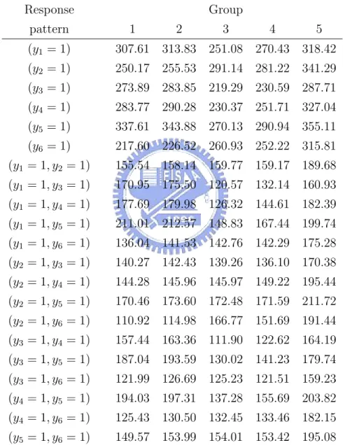
when sparseness occurs, we substitute the second-order marginal frequen-cies for original contingency table. Then, if the LCR model is rejected based on the use of the first- and second-order marginals, it could be concluded that the model does not hold in the joint frequencies either. Notationally set-up of the frequencies of the first- and second-order marginals may tabu-lated as Table 4. The rows of Table 4 are constituted by the following first-and second-order marginals :

   P r(Yij = s ; φ) for j = k P r(Yij = s, Yik = t ; φ) for j 6= k where k = 1,. . . , m; j = k,. . . , m ; s = 1,. . . , Kk − 1 ; t = 1,. . . , Kj − 1; φ = (β, γ, α).

The summation across the frequencies associated with the response pat-terns to obtain the marginal proportions represents a transformation of the frequencies in the multinomial vector π = (π1, π2,. . . , πk∗), which can be

implemented via multiplication by a matrix H.

The new Ohj and Ehj of three situations are as follows :

By matrix H, We can transform the original observed frequency table into new observed frequency table for each situation. Then, O∗

hj is hth row and

jth column of new observed frequency table. In the same way, We can

transform the original expected frequency table into new expected frequency table for each situation. And E∗

hj is hth row and jth column of new expected

frequency table.

Hence, the new test statistic is

T∗ 1 = K∗∗∗ X h=1 g X j=1 (O∗ hj − Ehj∗ )2 E∗ hj (7) where K∗∗∗ ₌PM m=1(Km− 1) + P_{M −1} m=1 h (Km− 1) × P_M m0_=m+1(Km0 − 1) i is the total number of response pattern of the first- and second-order marginals.

Similar to the Theorem 1, we rewrite the theorem as follows :

Theorem 2 Under LCR assumptions (1), (2), and (3), the distribution of

T∗ 1 will be asymptotically (N → ∞) K∗∗∗_g X i=1 λ∗_iχ2_1i where λ∗0

i s are the eigenvalues of the matrix

P (T∗ 1) = ZNTHSNT P (T1)SNHTZNT; i = 1,. . . , K∗ _{× g. Here,} P_(T 1) is mentioned in section 3.1. ZN is a

K∗∗∗_{g × K}∗∗∗_{g diagonal matrix with elements √}1

E∗ hj

, for h = 1,. . . , k∗∗∗_,

j = 1,. . . , g. SN is a K∗g × K∗g diagonal matrix with elements

p

h = 1,. . . , k∗_{, j = 1,. . . , g. The detailed proof of Theorem 2 can be found in}

Appendix C.

In order to estimate the large sample distribution of T∗

1 , we must

cal-culate the eigenvalues of the matrix P(T∗

1). Here, we substitute \ P (T∗ 1) = ˆ ZT NH ˆSNT \ P (T1) ˆSNHTZˆNT for P (T∗

1) and calculate the eigenvalues of the

ma-trix \P(T∗

1). Then, the nominal distribution will be

P_K∗∗∗_g i=1 λˆ∗iχ21i, where ˆλ∗ 0 i s are eigenvalues of \P(T∗ 1) .

Under sparse situation, we rewrite test statistic T2 and T3 as follow:

T∗ 2 = Wn∗ £ ZT nHSnT(IK∗_g− qqT − BJ−1BT)−1S_nHTZ_n ¤₋₁ W∗ n and T₃∗ = W_n∗£Z_nTHS_nT(IK∗_g− BJ−1BT)−1S_nHTZ_n ¤₋₁ W_n∗

Where Wn is a K∗∗∗g × 1 vector with elements Whj =

O∗ hj−Ehj∗ √ E∗ hj , for h = 1,. . . , k∗∗∗_{, j = 1,. . . , g. The asymptotic distributions to T}∗

2 and T3∗ are

4

Simulation Studies

4.1

Generated data from the LCR model

Here, we are going to simulate two major situations to discuss. One is ”balance” and the other is ”unbalance”. ”Balance” means the contingency table is not sparse and ”unbalance” means contingency table is sparse.

In balanced case, we simulate three-class LCR with five-two level mea-sured indicator, two covariates associated with conditional probabilities, two covariates associated with latent prevalence and sample size is 2500 (i.e., J = 3, M = 5, K1 =. . . = K5 = 2, P = L = 2, N = 2500). Then, βpj , which are

the model parameters, can be determined randomly by setting βpj = k1Uj

, Uj ∼ U(0, 1) , for each p ∈ {0, 1,. . . , P }; j = 1,. . . , (J − 1). k1 is

con-stant such that PP_p=1PJ−1_j=1 βpj equal the preselected total. Similarly, we

can use the same way to determine {γjmk, j = 1,. . . , (J − 1)} for all m,

k and {αqmk, m = 1,. . . , M ; k = 1,. . . , (Km− 1)} for all q. Here, we

set the parametric values of PL_l=1PM_m=1αlm and

P_m i=1 P_J j=1α0 as 1 and of PP_p=1PJ−1_j=1 βpj and P_J−1

j=1 β0 as 0.6. And observable Yi0s are generated

with 100 replications. Table 5 shows the values of α0 and αlm. Table 6 shows

the values of β0 and βpj.

The covariates associated with conditional probabilities (zim1, zim2), m =

1,. . . , 5 and latent prevalences (xi1, xi2) are generated as follows:

For each m

zim1∼ Bernoulli(0.4), zim2 ∼ Normal(50, 5) i = 1 ∼ 500

zim1∼ Binomial(14, 0.6), zim2 ∼ Unif orm(1, 10) i = 1001 ∼ 1500

zim1∼ Binomial(6, 0.4), zim2 ∼ Exponential(6) i = 1501 ∼ 2000

zim1∼ P oisson(3), zim2∼ Unif otm(20, 30) i = 2001 ∼ 2500

and covariates associated with latent prevalences are generated as

xi1∼ Bernoulli(0.6), xi2∼ Normal(0, 1) i = 1,. . . , 2500

In unbalanced case, we simulate five-class LCR with six-two level mea-sured indicator, two covariates associated with conditional probabilities, two covariates associated with latent prevalence and sample size is 2500 (i.e., J =

5, M = 6, K1 =. . . = K6 = 2, P = L = 2, N = 2500, g = 5). Here, we set

the parametric values of PL_l=1PM_m=1αlm and

P_m i=1 P_J j=1α0 as 1.5 and of P_P p=1 P_J−1 j=1 βpj and P_J−1

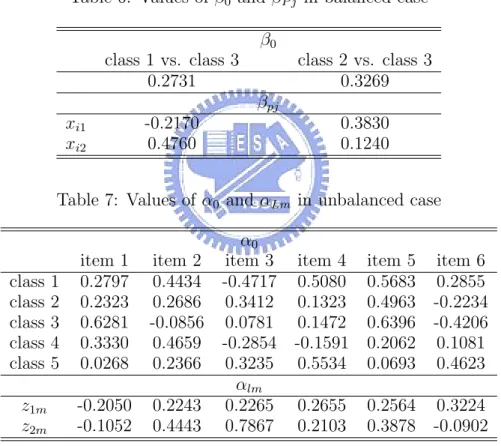
j=1 β0 as 0.8. Table 7 shows the values of α0 and

αlm. Table 8 shows the values of β0 and βpj. Then, the covariates associated

with conditional probabilities (zim1, zim2), m = 1,. . . , 5 and latent prevalences

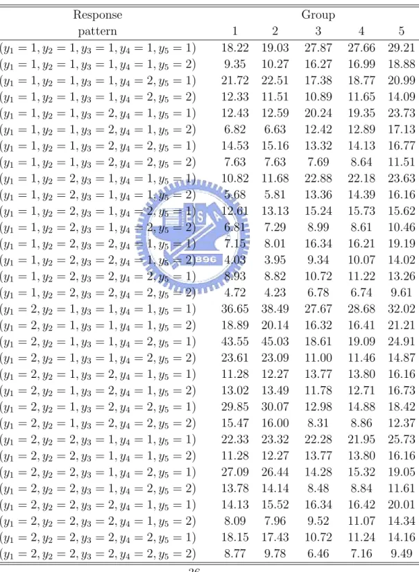
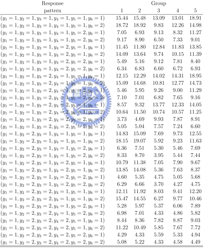
(xi1, xi2) are generated by the same ways in balanced case. Table 9 is the

averaged O’s over 100 simulations in the contingency table forming by all response patterns in balanced case and Table 10 is the averaged O’s over 100 simulations in unbalanced case. Table 11 is table 10 after combining as first-and second order marginals.

The simulation results are represented from Table 12 to Table 17. Ac-cording to the results of balanced case, test statistics of fanny are well ap-proximated to nominal distribution. Nevertheless, behaviors of three test statistics of clara are not as good as behaviors of fanny, because the values of clara are obviously lower than nominal distribution.

of test statistics of fanny are higher than nominal distribution. While the values of test statistics of clara are lower than nominal distribution.

4.2

Assess power of the proposed test statistics

The simulations considered thus far have demonstrated that the test sta-tistic have well defined distributions under the null hypotheses that the LCR model holds. To examine the power of the proposed test statistics, data were generated the same as section 4.1. Then, we use a simpler model to fit the data which were generated from a complicated model.

The selected sample size is 2500 and Y0

is are generated with 100

replica-tion. In balanced case, we use two-class LCR with five-two level measured indicator, one covariate associated with conditional probabilities, one covari-ates associated with latent prevalence (i.e., J = 2, M = 5, K1 =. . . = K5 =

2, P = L = 1) and divide the population into three groups to fit alter-native model. The covariates associated with conditional probabilities zim1

,m = 1,. . . , 5 and latent prevalences xi1 are generated as follows :

For each m

zim2∼ Normal(20, 5) i = 1 ∼ 800

zim2∼ Gamma(4, 2) i = 801 ∼ 1600

zim2∼ P oisson(15) i = 1601 ∼ 2500

and covariates associated with latent prevalences are generated as

xi2∼ Normal(0, 1) i = 1,. . . , 2500

In unbalanced case, we use three-class LCR with six-two level measured indicator, one covariate associated with conditional probabilities, one

covari-ates associated with latent prevalence(i.e., J = 3, M = 6, K1 =. . . = K6 =

2, P = L = 1) and divide the population into three groups to fit alter-native model. The covariates associated with conditional probabilities zim1

,m = 1,. . . , 6 and latent prevalences xi1are generated as the same in balanced

case.

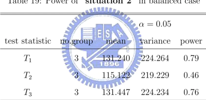
Table 18 presents the results of clara method in balanced case. Three test statistics virtually have no power. This method seems to cluster the population unsuitably under the balanced situation. Table 19 and Table 20 present the results of fanny method in balanced case. In Table 19, T1 and

T3 have higher power in detecting the difference between fitted model and

alternative model. While T2 have comparably lower power. In Table 20,

power of T1 is lower than powers of T2 and T3. Table 21, Table 22 and Table

23 present the results of clara and fanny method in unbalanced case. The conclusions are similar to balanced case.

5

Discussion

In this paper, we use the latent class regression model to fit the relationship between a latent class outcome and latent factor predictors. We propose the goodness-of-fit test statistic to assess the adequacy of the model. The number of the group is determined before forming the contingency table. Then, we use two clustering methods, clara and fanny, to cluster the population.

The fanny method is a good approach for our grouping the population of the LCR model. Under fanny method, situation 2 is well than situation 3. So we suggest using method of situation 2. But fanny method is sensitive to covariates which are selected to do the clustering. There is a serious influence on the results of the cluster. Therefore, when we select covariates to do the clustering, we should select carefully to avoid the inappropriate results.

Appendix A: Silhouette coefficient

For each object i, we denote A the cluster to which it belongs, and compute

a(i) := 1 |A| − 1

X

j∈A,j6=i

d(i, j)

It is the average dissimilarity of i to all other objects of A. Here, d(i, j) is defined as

d(i, j) = P_p f =1δ (f ) ij d (f ) ij P_p f =1δ (f ) ij ∈ [0, 1] where

d(f )_ij = contribution of variable f to d(i, j), which depends on its type : 1. f binary or nominal : d(f )_ij = 0 if xif = xjf, and d(f )ij = 1 otherwise,

2. f interval-scaled : d(f )_ij = |xif−xjf|

maxhxhf−minhxhf,

3. f ordinal or ratio-scaled : compute ranks rif and zif = _maxrif_hr−1_hf−1 and

treat these zif as interval-scaled,

and

δ_ij(f ) = weight of variable f : 1. δ_ij(f ) = 0 if xif or xjf is missing,

2. δ_ij(f ) = 0 if xif = xjf = 0 and variable f is asymmetric binary,

3. δ_ij(f ) = 1 otherwise. and p is number of variables.

Now consider any cluster C different from A and put

d(i, C) := 1 |C|

X

j∈C

It is the average dissimilarity of i to all other objects of C.

After computing d(i, C) for all clusters C 6= A we take the smallest of those:

b(i) := min

C6=Ad(i, C).

The cluster B which attains this minimum [that is, d(i, B) = b(i)] is called the neighbor of object i. This is the second-best cluster for object i.

The silhouette value s(i) of the object i is defined as

s(i) := b(i) − a(i) max{a(i), b(i)}.

Appendix B: Proof of theorem 1

Then regular conditions of theorem 4.2 in Moor and Spruill are satisfied as follows :

1. Under (φN, ϕ), φN − φ0 = oK∗∗(1) and ϕn = ϕ(x, z). Every vertex

y(φ) of every cell Iσ(φ) is a continuous RM-valued function of φ in a

neighborhood of φ0.

2. For each σ, Pσ(φ, ϕ) is continuous in (φ, ϕ) and continuously

differen-tiable in (φ) in a neighborhood of (φ0, ϕ0). Moreover,

P_K∗∗_g

σ=1 Pσ = 1

and Pσ > 0 for each σ.

3. F (y) = F (y|φ0) is continuous at every vertex y(φ0) of every cell Iσ(φ0).

As N → ∞, supy|F (y|φN) − F (y)| → 0.

4. K(φ) = S(φ)S(φ)T _{for an K}∗∗_{g × K}∗∗_{g matrix S(φ) with entries}

con-tinuous in φ at φ0. 5. Under φN N1/2_(φ N − φ0) = N−1/2 N X i=1 h(Yi, φN) + Aγ+ oK∗∗(1)

for some g × K∗∗_{matrix A and measurable function h(y, φ) from R}M_×

RK∗∗ to Rg _satisfying E [h(Y, φN)|φN] = 0 E£h(Y, φN)h(Y, φN)T|φN ¤ = L(φN)

where L(φN) is a g × g matrix converging to the finite and matrix

6. g ≤ K∗_{g and the matrix with entries ∂p}

i/∂φj has rank g.

7. logf (y|φ) is differentiable with respect to φ at φ0. The matrix J is pd

and J12 is finite. (∂/∂φ)F (y|φ) may be evaluated by differentiating

f (y|φ) under the integral sign for all y and φ = φ0.

8. n1/2_{( ˆφ} n− φ0) = n−1/2 P_n i=1J−1 ∂logf (Yi |ηn) ∂φ + J−1J12γ + op(1). Here J is

the information matrix for F (y|φ) at φ0.

J = E · (∂logf ∂φ )( ∂logf ∂φ ) T ¸ , J12 is the m × p matrix J12 = E · (∂logf ∂φ )( ∂logf ∂η ) T ¸ .

9. J − BT_{B is pd, where matrix B has (i, j)th entry p}−1/2 i ∂φ∂pij .

Appendix C: Distributions of test statistic T∗

1, T2∗ and T3∗

N = total number of individuals

h = 1, 2,. . . , K∗_{, where K}∗ ₌QM m=1km

j = 1, 2,. . . , g, where g = number of groups

VN = K∗g × 1 vector VN =                       v11 ... v1g ... ... vK∗₁ ... vK∗_g                       , where vhj = Ohj_p− Ehj Ehj

Ehj = expected number of observation in (h, j)

TN = VNTKNVN =k SNTVN k2= P_K∗ h=1 P_g j=1(Ohj − Ehj)2 where KN =                       E11 . .. 0 E1g . .. . .. EK∗₁ 0 . .. EK∗_g                      

and KN = SNSNT So SN =                       √ E11 . .. 0 p E1g . .. . .. √ EK∗₁ 0 . .. p EK∗_g                      

By theorem 4.2 in Moore & Spruill

ST NVN → N(µ, Σd 0) where Σ0 = SNT(IK∗_g− qqT − BJ−1BT)S_N   ···k SNTVN k2= VNTSNVN → Σd K ∗_g i=1λiχ21i where λ0 is are eigenvalues of Σ0   Let K∗∗∗ ₌PM m=1(Km− 1) + P_M i6=j=1(Ki− 1)(Kj− 1) WN = K∗∗∗× 1 vector WN =                       w11 ... w1g ... ... wK∗∗∗₁ ... wK∗∗∗_g                       , where wsj = O∗ sj_p− Esj∗ E∗ sj

O∗

sj = number of observation in (s, j) after combining.

E∗

sj = expected number of observation in (s, j) after combining.

Let WN = H∗SNTVN H∗_K∗∗∗_g×K∗∗∗_g =      H 0 . .. 0 H     , where H is matrix which is mentioned in second-order. So WN = H∗SNTVN → N(Hd ∗µ, H∗Σ0H∗ T ) and H∗_Σ 0H∗ T = H∗_ST N(IK∗_g − qqT − BJ−1BT)S_NH∗ T Let W∗ N = ZNTWN, where ZN is a K∗∗∗g × K∗∗∗g matrix. ZN =                       1/pE∗ 11 . .. 0 1/pE∗ 1g . .. . .. 1/pE∗ K∗∗∗₁ 0 . .. 1/pE∗ K∗∗∗_g                       So W∗ N = ZNTWN → N(Zd NTH∗µ, ZNTH∗Σ0H∗ T ZN) ⇒ W∗T N WN∗ = P_K∗∗∗ s=1 P_g j=1 (O∗ sj−Esj∗)2 E∗ sj ∼ P_K∗∗∗ i=1 λ∗iχ21i where λ∗0 i s is eigenvalues of Σ∗ = ZNTΣZN

References

[1] Agresti, A. (1984). Analysis of Catagorical Data. New York: J.Wiley and Sons.

[2] Agresti,A.,Yang,M.C. (1987).An Empirical Investigation of Some Effects of Sparseness in Contingency Tables.

Computa-tional Statistics and Data Analysis.5:9-21.

[3] Bandeen-Roche,K.,Miglioretti,D.L.,Zeger,

S.L.,Rathouz,P.J. (1997).Latent Variable Regression For Multiple Discrete Outcome. Journal of the American Statistical

Association. 92: 1375-1386.

[4] Batholomew, D.J. (1987).Latent Variable Model and Factor

Analysis. London: Charles Griffin & Co. Ltd.

[5] Demster, A.P,Laird, N.M.,Rubin, D.B (1977). Maximum likelihood from incomplete data via the EM algorithm. Journal

of the Royal Statistical Society, Series B ;39:1-38.

[6] Drust,M.C.,Donsker.(1980).Vapnik-Chervonenkis classes

and chi-square tests of fit with random cells; Unpublished doctoral dissertation, Department of Mathematics, M.I.T., Cambridge,MA.

[7] Formann, A.K. (1992).Linear logistic latent class analysis for polytomous data. Journal of the American Statistical

[8] Goodman, L.A. (1974). Exploratory latent structure analysis using both identifiable and unidentifiable models. Biomertrika. 61:215-231

[9] Hosmer, D.W.,Lemeshow,s. Applied Logistic Regression. New York: John Wiley & Sons.

[10] Huang, G.H.,Bandeen-Roche, L. Latent variable regression with covariate effects on underlying and measured variables: an approach of analyzing multiple polytomous surrogates. Submit-ted for publication.

[11] Kuo, H.Y. (2004). Goodness-of-fit Test for Latent Class Re-gression Model. To be submitted.

[12] Lemeshow, S.,Hosmer, D.W. (1982). The Use of Goodness-of-fit Statistics in the Development of Logistic Regression Mod-els.American journal of Epidemiology. 115:92-106

[13] McCullagh, P.,Nelder, J.A. (1989). Generalized Linear

Models, 2nd edition. London: Chapman and Hall.

[14] Moore,D.S.,Spruill,M.C.(1975). Unified Large-sample The-ory of General Chi-squared Statistic for Tests of Fit. Annals of

Statistics. 3:599-616.

[15] Reiser,M.,Lin,Y.(1999). A Goodness-of-Fit Test for the Latent Class Model When Expected Frequencies are Small. Sociological

[16] Struyf,A.,Hubert,M.,Rousseeuw,P.J.(1996).Clustering in an Object-Oriented Environment. Journal of Statistical

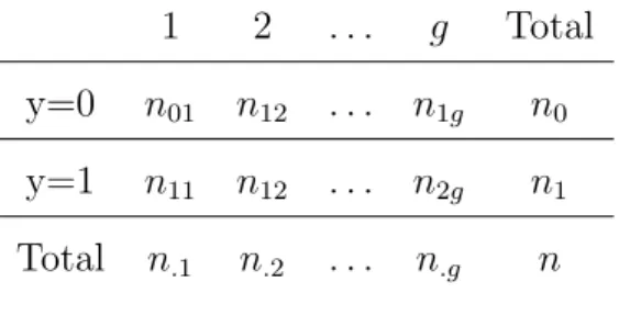
Table 1: Notational set-up of the frequencies in logistic regression model

1 2 . . . g Total

y=0 n01 n12 . . . n1g n0

y=1 n11 n12 . . . n2g n1

Total n.1 n.2 . . . n.g n

Table 2: Notational set-up of the frequencies in LCR model

1 2 . . . g (y1 = 1, y2 = 1,. . . , ym = 1) O11 O12 . . . O1g (y1 = 1, y2 = 1,. . . , ym = 2) O21 O22 . . . O2g ... ... ... ... (y1 = 1, y2 = 1,. . . , ym = km) Om1 Om2 . . . Omg ... ... ... ... (y1 = k1, y2 = k2,. . . , ym = km) Ok∗₁ O_K∗₂ . . . O_K∗_g n1 n2 . . . ng

Table 3: Interpretation of the silhouette coefficient for partitioning method

SC Proposed Interpretation

0.71-1.00 A strong structure has been found.

0.51-0.70 A reasonable structure has been found

0.26-0.50 The structure is weak and could be artificial, try additional method

Table 4: Notational set-up of the frequencies of first- and second-order mar-ginals 1 2 . . . g (y1 = 1) O11 O12 . . . O1g ... ... ... ... (y1 = k1− 1) Oh11 Oh12 . . . Oh1g (y2 = 1) Oh21 Oh22 . . . Oh2g ... ... ... ... (y2 = k2− 1) Oh31 Oh32 . . . Oh3g ... ... ... ... (yM = 1) Oh41 Oh42 . . . Oh4g ... ... ... ... (yM = kM − 1) Oh51 Oh52 . . . Oh5g (y1 = 1, y2 = 1) Oh61 Oh62 . . . Oh6g (y1 = 1, y2 = 2) Oh71 Oh72 . . . Oh7g ... ... ... ... (y1 = 1, y2 = k2− 1) Oh81 Oh82 . . . Oh8g (y1 = 2, y2 = 1) Oh91 Oh92 . . . Oh9g ... ... ... ... (y1 = k1− 1, y2 = k2− 1) Oh101 Oh102 . . . Oh10g ... ... ... ... (yM −1 = 1, yM = 1) Oh111 Oh112 . . . Oh11g ... ... ... ... (yM −1= kM −1− 1, yM = kM − 1) Ok∗∗∗₁ O_K∗∗∗₂ . . . O_K∗∗∗_g n1 n2 . . . ng Note: h1 = k1 − 1, h2 = (k1 − 1) + 1, h3 = P₂ i=1(ki− 1) h4 = hP_{M −1} i=1 (ki− 1) i + 1, h5 = P_M i=1(ki− 1), h6 = hP_M i=1(ki− 1) i + 1 h7 = hP_M i=1(ki− 1) i + 2, h8 = hP_M i=1(ki− 1) i + (k2− 1), h9 = hP_M i=1(ki− 1) i + k2 h10 = hP_M i=1(ki− 1) i + (k1− 1)(k2− 1) h =hPM (k − 1) i +hPM −1 (k − 1)(k − 1) i + 1

Table 5: Values of α0 and αLm in balanced case

α0

item 1 item 2 item 3 item 4 item 5

class 1 -0.6012 0.6358 0.2786 -0.3152 0.5294 class 2 0.1289 0.3371 0.1878 0.3102 0.3829 class 3 0.2698 0.0271 -0.5336 0.3746 -0.3508 αlm z1m -0.1741 -0.1904 0.1923 0.2254 0.2177 z2m 0.1984 0.2835 0.2014 -0.2836 0.1674

Table 6: Values of β0 and βP j in balanced case

β0

class 1 vs. class 3 class 2 vs. class 3

0.2731 0.3269

βpj

xi1 -0.2170 0.3830

xi2 0.4760 0.1240

Table 7: Values of α0 and αLm in unbalanced case

α0

item 1 item 2 item 3 item 4 item 5 item 6

class 1 0.2797 0.4434 -0.4717 0.5080 0.5683 0.2855 class 2 0.2323 0.2686 0.3412 0.1323 0.4963 -0.2234 class 3 0.6281 -0.0856 0.0781 0.1472 0.6396 -0.4206 class 4 0.3330 0.4659 -0.2854 -0.1591 0.2062 0.1081 class 5 0.0268 0.2366 0.3235 0.5534 0.0693 0.4623 αlm z1m -0.2050 0.2243 0.2265 0.2655 0.2564 0.3224 z2m -0.1052 0.4443 0.7867 0.2103 0.3878 -0.0902

Table 8: Values of β0 and βP j in unbalanced case

β0

class 1 vs. class 5 class 2 vs. class 5 class 3 vs. class 5 class 4 vs. class5

0.2510 0.3041 0.0413 0.2035

βpj

xi1 0.1655 -0.2943 0.1719 0.3683

Table 9: Observed contingency table of balanced case, averaging over 100 simulations Response Group pattern 1 2 3 4 5 (y1 = 1, y2 = 1, y3 = 1, y4 = 1, y5 = 1) 18.22 19.03 27.87 27.66 29.21 (y1 = 1, y2 = 1, y3 = 1, y4 = 1, y5 = 2) 9.35 10.27 16.27 16.99 18.88 (y1 = 1, y2 = 1, y3 = 1, y4 = 2, y5 = 1) 21.72 22.51 17.38 18.77 20.99 (y1 = 1, y2 = 1, y3 = 1, y4 = 2, y5 = 2) 12.33 11.51 10.89 11.65 14.09 (y1 = 1, y2 = 1, y3 = 2, y4 = 1, y5 = 1) 12.43 12.59 20.24 19.35 23.73 (y1 = 1, y2 = 1, y3 = 2, y4 = 1, y5 = 2) 6.82 6.63 12.42 12.89 17.13 (y1 = 1, y2 = 1, y3 = 2, y4 = 2, y5 = 1) 14.53 15.16 13.32 14.13 16.77 (y1 = 1, y2 = 1, y3 = 2, y4 = 2, y5 = 2) 7.63 7.63 7.69 8.64 11.51 (y1 = 1, y2 = 2, y3 = 1, y4 = 1, y5 = 1) 10.82 11.68 22.88 22.18 23.63 (y1 = 1, y2 = 2, y3 = 1, y4 = 1, y5 = 2) 5.68 5.81 13.36 14.39 16.16 (y1 = 1, y2 = 2, y3 = 1, y4 = 2, y5 = 1) 12.61 13.13 15.24 15.73 15.62 (y1 = 1, y2 = 2, y3 = 1, y4 = 2, y5 = 2) 6.81 7.29 8.99 8.61 10.46 (y1 = 1, y2 = 2, y3 = 2, y4 = 1, y5 = 1) 7.15 8.01 16.34 16.21 19.19 (y1 = 1, y2 = 2, y3 = 2, y4 = 1, y5 = 2) 4.03 3.95 9.34 10.07 14.02 (y1 = 1, y2 = 2, y3 = 2, y4 = 2, y5 = 1) 8.93 8.82 10.72 11.22 13.26 (y1 = 1, y2 = 2, y3 = 2, y4 = 2, y5 = 2) 4.72 4.23 6.78 6.74 9.61 (y1 = 2, y2 = 1, y3 = 1, y4 = 1, y5 = 1) 36.65 38.49 27.67 28.68 32.02 (y1 = 2, y2 = 1, y3 = 1, y4 = 1, y5 = 2) 18.89 20.14 16.32 16.41 21.21 (y1 = 2, y2 = 1, y3 = 1, y4 = 2, y5 = 1) 43.55 45.03 18.61 19.09 24.91 (y1 = 2, y2 = 1, y3 = 1, y4 = 2, y5 = 2) 23.61 23.09 11.00 11.46 14.87 (y1 = 2, y2 = 1, y3 = 2, y4 = 1, y5 = 1) 11.28 12.27 13.77 13.80 16.16 (y1 = 2, y2 = 1, y3 = 2, y4 = 1, y5 = 2) 13.02 13.49 11.78 12.71 16.73 (y1 = 2, y2 = 1, y3 = 2, y4 = 2, y5 = 1) 29.85 30.07 12.98 14.88 18.42 (y1 = 2, y2 = 1, y3 = 2, y4 = 2, y5 = 2) 15.47 16.00 8.31 8.86 12.37 (y1 = 2, y2 = 2, y3 = 1, y4 = 1, y5 = 1) 22.33 23.32 22.28 21.95 25.73 (y1 = 2, y2 = 2, y3 = 1, y4 = 1, y5 = 2) 11.28 12.27 13.77 13.80 16.16 (y1 = 2, y2 = 2, y3 = 1, y4 = 2, y5 = 1) 27.09 26.44 14.28 15.32 19.05 (y1 = 2, y2 = 2, y3 = 1, y4 = 2, y5 = 2) 13.78 14.14 8.48 8.84 11.61 (y1 = 2, y2 = 2, y3 = 2, y4 = 1, y5 = 1) 14.13 15.52 16.34 16.42 20.01 (y1 = 2, y2 = 2, y3 = 2, y4 = 1, y5 = 2) 8.09 7.96 9.52 11.07 14.34 (y1 = 2, y2 = 2, y3 = 2, y4 = 2, y5 = 1) 18.15 17.43 10.72 11.24 14.16 (y1 = 2, y2 = 2, y3 = 2, y4 = 2, y5 = 2) 8.77 9.78 6.46 7.16 9.49

Table 10: Observed contingency table of unbalanced case, averaging over 100 simulations Response Group pattern 1 2 3 4 5 (y1 = 1, y2 = 1, y3 = 1, y4 = 1, y5 = 1, y6 = 1) 15.44 15.48 13.09 13.01 18.91 (y1 = 1, y2 = 1, y3 = 1, y4 = 1, y5 = 1, y6 = 2) 18.72 18.92 9.83 12.26 14.98 (y1 = 1, y2 = 1, y3 = 1, y4 = 1, y5 = 2, y6 = 1) 7.05 6.93 9.13 8.32 11.27 (y1 = 1, y2 = 1, y3 = 1, y4 = 1, y5 = 2, y6 = 2) 9.17 8.90 6.50 7.33 9.01 (y1 = 1, y2 = 1, y3 = 1, y4 = 2, y5 = 1, y6 = 1) 11.45 11.80 12.84 11.83 13.85 (y1 = 1, y2 = 1, y3 = 1, y4 = 2, y5 = 1, y6 = 2) 14.09 13.64 9.74 10.15 11.39 (y1 = 1, y2 = 1, y3 = 1, y4 = 2, y5 = 2, y6 = 1) 5.49 5.16 9.12 7.81 8.40 (y1 = 1, y2 = 1, y3 = 1, y4 = 2, y5 = 2, y6 = 2) 6.34 6.83 6.60 6.72 6.93 (y1 = 1, y2 = 1, y3 = 2, y4 = 1, y5 = 1, y6 = 1) 12.15 12.29 14.02 14.31 18.95 (y1 = 1, y2 = 1, y3 = 2, y4 = 1, y5 = 1, y6 = 2) 15.09 14.68 10.81 12.77 14.73 (y1 = 1, y2 = 1, y3 = 2, y4 = 1, y5 = 2, y6 = 1) 5.46 5.95 9.26 9.00 11.29 (y1 = 1, y2 = 1, y3 = 2, y4 = 1, y5 = 2, y6 = 2) 7.10 7.01 6.82 7.65 9.16 (y1 = 1, y2 = 1, y3 = 2, y4 = 2, y5 = 1, y6 = 1) 8.57 9.32 13.77 12.33 14.05 (y1 = 1, y2 = 1, y3 = 2, y4 = 2, y5 = 1, y6 = 2) 10.64 11.50 10.74 10.57 11.25 (y1 = 1, y2 = 1, y3 = 2, y4 = 2, y5 = 2, y6 = 1) 3.73 4.69 9.93 7.87 8.91 (y1 = 1, y2 = 1, y3 = 2, y4 = 2, y5 = 2, y6 = 2) 5.05 5.04 7.57 7.24 6.60 (y1 = 1, y2 = 2, y3 = 1, y4 = 1, y5 = 1, y6 = 1) 14.83 15.09 7.69 9.73 12.55 (y1 = 1, y2 = 2, y3 = 1, y4 = 1, y5 = 1, y6 = 2) 18.15 19.07 5.92 9.23 11.63 (y1 = 1, y2 = 2, y3 = 1, y4 = 1, y5 = 2, y6 = 1) 6.36 7.51 5.30 5.46 7.69 (y1 = 1, y2 = 2, y3 = 1, y4 = 1, y5 = 2, y6 = 2) 8.33 8.70 3.95 5.44 7.44 (y1 = 1, y2 = 2, y3 = 1, y4 = 2, y5 = 1, y6 = 1) 10.79 11.38 7.05 7.90 9.67 (y1 = 1, y2 = 2, y3 = 1, y4 = 2, y5 = 1, y6 = 2) 13.85 14.08 5.36 7.63 8.37 (y1 = 1, y2 = 2, y3 = 1, y4 = 2, y5 = 2, y6 = 1) 4.60 5.35 4.75 5.05 5.68 (y1 = 1, y2 = 2, y3 = 1, y4 = 2, y5 = 2, y6 = 2) 6.29 6.66 3.70 4.27 4.75 (y1 = 1, y2 = 2, y3 = 2, y4 = 1, y5 = 1, y6 = 1) 12.11 11.92 8.03 9.41 12.20 (y1 = 1, y2 = 2, y3 = 2, y4 = 1, y5 = 1, y6 = 2) 15.47 14.55 6.27 9.77 10.46 (y1 = 1, y2 = 2, y3 = 2, y4 = 1, y5 = 2, y6 = 1) 5.28 5.97 5.37 6.06 7.89 (y1 = 1, y2 = 2, y3 = 2, y4 = 1, y5 = 2, y6 = 2) 6.98 7.01 4.33 4.86 5.82 (y1 = 1, y2 = 2, y3 = 2, y4 = 2, y5 = 1, y6 = 1) 8.44 8.36 7.82 8.87 9.03 (y1 = 1, y2 = 2, y3 = 2, y4 = 2, y5 = 1, y6 = 2) 11.22 10.49 5.85 7.67 7.72 (y1 = 1, y2 = 2, y3 = 2, y4 = 2, y5 = 2, y6 = 1) 4.29 4.33 5.59 5.33 4.94 (y1 = 1, y2 = 2, y3 = 2, y4 = 2, y5 = 2, y6 = 2) 5.08 5.22 4.33 4.58 4.49

Response Group pattern 1 2 3 4 5 (y1 = 2, y2 = 1, y3 = 1, y4 = 1, y5 = 1, y6 = 1) 9.01 9.66 11.17 10.43 15.26 (y1 = 2, y2 = 1, y3 = 1, y4 = 1, y5 = 1, y6 = 2) 11.23 11.75 8.26 8.44 11.51 (y1 = 2, y2 = 1, y3 = 1, y4 = 1, y5 = 2, y6 = 1) 4.51 4.58 7.26 6.72 9.62 (y1 = 2, y2 = 1, y3 = 1, y4 = 1, y5 = 2, y6 = 2) 5.49 5.70 5.44 5.76 6.74 (y1 = 2, y2 = 1, y3 = 1, y4 = 2, y5 = 1, y6 = 1) 6.75 7.12 10.20 8.85 11.20 (y1 = 2, y2 = 1, y3 = 1, y4 = 2, y5 = 1, y6 = 2) 8.18 8.78 7.77 7.69 9.00 (y1 = 2, y2 = 1, y3 = 1, y4 = 2, y5 = 2, y6 = 1) 3.23 3.06 6.83 5.97 7.04 (y1 = 2, y2 = 1, y3 = 1, y4 = 2, y5 = 2, y6 = 2) 4.12 4.12 5.48 4.81 5.27 (y1 = 2, y2 = 1, y3 = 2, y4 = 1, y5 = 1, y6 = 1) 7.00 7.00 12.23 11.38 15.34 (y1 = 2, y2 = 1, y3 = 2, y4 = 1, y5 = 1, y6 = 2) 9.17 9.09 8.22 9.15 11.60 (y1 = 2, y2 = 1, y3 = 2, y4 = 1, y5 = 2, y6 = 1) 3.30 3.81 8.26 7.25 9.63 (y1 = 2, y2 = 1, y3 = 2, y4 = 1, y5 = 2, y6 = 2) 4.39 4.21 5.67 5.44 7.44 (y1 = 2, y2 = 1, y3 = 2, y4 = 2, y5 = 1, y6 = 1) 5.41 5.75 11.05 10.03 10.72 (y1 = 2, y2 = 1, y3 = 2, y4 = 2, y5 = 1, y6 = 2) 7.56 6.82 8.74 8.39 8.98 (y1 = 2, y2 = 1, y3 = 2, y4 = 2, y5 = 2, y6 = 1) 2.37 2.38 8.61 6.58 7.00 (y1 = 2, y2 = 1, y3 = 2, y4 = 2, y5 = 2, y6 = 2) 2.91 3.56 6.18 5.16 5.26 (y1 = 2, y2 = 2, y3 = 1, y4 = 1, y5 = 1, y6 = 1) 9.07 9.53 6.23 6.47 9.71 (y1 = 2, y2 = 2, y3 = 1, y4 = 1, y5 = 1, y6 = 2) 10.97 11.75 4.43 6.16 8.27 (y1 = 2, y2 = 2, y3 = 1, y4 = 1, y5 = 2, y6 = 1) 3.86 4.44 4.37 4.02 6.37 (y1 = 2, y2 = 2, y3 = 1, y4 = 1, y5 = 2, y6 = 2) 5.25 5.35 3.33 3.84 4.82 (y1 = 2, y2 = 2, y3 = 1, y4 = 2, y5 = 1, y6 = 1) 6.47 6.54 5.90 5.83 7.37 (y1 = 2, y2 = 2, y3 = 1, y4 = 2, y5 = 1, y6 = 2) 8.04 9.00 4.54 5.62 6.07 (y1 = 2, y2 = 2, y3 = 1, y4 = 2, y5 = 2, y6 = 1) 3.08 3.06 4.30 4.11 4.64 (y1 = 2, y2 = 2, y3 = 1, y4 = 2, y5 = 2, y6 = 2) 3.68 3.91 3.21 3.73 3.89 (y1 = 2, y2 = 2, y3 = 2, y4 = 1, y5 = 1, y6 = 1) 7.04 7.49 6.43 6.93 9.60 (y1 = 2, y2 = 2, y3 = 2, y4 = 1, y5 = 1, y6 = 2) 8.58 9.04 4.65 6.24 8.12 (y1 = 2, y2 = 2, y3 = 2, y4 = 1, y5 = 2, y6 = 1) 2.96 2.85 4.61 4.96 5.87 (y1 = 2, y2 = 2, y3 = 2, y4 = 1, y5 = 2, y6 = 2) 4.25 4.05 3.49 3.91 4.75 (y1 = 2, y2 = 2, y3 = 2, y4 = 2, y5 = 1, y6 = 1) 5.04 5.26 6.49 6.11 6.67 (y1 = 2, y2 = 2, y3 = 2, y4 = 2, y5 = 1, y6 = 2) 7.08 6.73 4.99 5.78 5.95 (y1 = 2, y2 = 2, y3 = 2, y4 = 2, y5 = 2, y6 = 1) 2.46 2.46 4.23 4.29 4.49 (y1 = 2, y2 = 2, y3 = 2, y4 = 2, y5 = 2, y6 = 2) 2.93 3.32 3.35 3.52 3.38

Table 11: Observed contingency table of first- and second-order marginals, averaging over 100 simulations

Response Group pattern 1 2 3 4 5 (y1 = 1) 307.61 313.83 251.08 270.43 318.42 (y2 = 1) 250.17 255.53 291.14 281.22 341.29 (y3 = 1) 273.89 283.85 219.29 230.59 287.71 (y4 = 1) 283.77 290.28 230.37 251.71 327.04 (y5 = 1) 337.61 343.88 270.13 290.94 355.11 (y6 = 1) 217.60 226.52 260.93 252.22 315.81 (y1 = 1, y2 = 1) 155.54 158.14 159.77 159.17 189.68 (y1 = 1, y3 = 1) 170.95 175.50 120.57 132.14 160.93 (y1 = 1, y4 = 1) 177.69 179.98 126.32 144.61 182.39 (y1 = 1, y5 = 1) 211.01 212.57 148.83 167.44 199.74 (y1 = 1, y6 = 1) 136.04 141.53 142.76 142.29 175.28 (y2 = 1, y3 = 1) 140.27 142.43 139.26 136.10 170.38 (y2 = 1, y4 = 1) 144.28 145.96 145.97 149.22 195.44 (y2 = 1, y5 = 1) 170.46 173.60 172.48 171.59 211.72 (y2 = 1, y6 = 1) 110.92 114.98 166.77 151.69 191.44 (y3 = 1, y4 = 1) 157.44 163.36 111.90 122.62 164.19 (y3 = 1, y5 = 1) 187.04 193.59 130.02 141.23 179.74 (y3 = 1, y6 = 1) 121.99 126.69 125.23 121.51 159.23 (y4 = 1, y5 = 1) 194.03 197.31 137.28 155.69 203.82 (y4 = 1, y6 = 1) 125.43 130.50 132.45 133.46 182.15 (y5 = 1, y6 = 1) 149.57 153.99 154.01 153.42 195.08