國
立
交
通
大
學
電信工程研究所
碩
士
論
文
正交頻率多工訊號之低複雜度峰均值降低方法
Low-Complexity PAPR Reduction Schemes for OFDM Systems
研 究 生:陳至寧
正交頻率多工訊號之低複雜度峰均值降低方法
Low-Complexity PAPR Reduction Schemes for OFDM Systems
研 究 生:陳至寧 Student:Chih-Ning Chen
指導教授:蘇育德 Advisor:Dr. Tu T. Su
國 立 交 通 大 學
電信工程研究所
碩 士 論 文
A ThesisSubmitted to Institute of Communication Engineering College of Electrical and Computer Engineering
National Chiao Tung University in partial Fulfillment of the Requirements
for the Degree of Master
in
Communication Engineering
August 2011
正交頻率多工訊號之低複雜度峰均值降低之方法 學生:陳至寧 指導教授:蘇育德 博士 國立交通大學電信工程研究所碩士班 摘 要 由 於 正 交 頻 率 多 工 (OFDM) 信 號 會 使 傳 送 時 間 訊 號 產 生 高 峰 均 值 (PAPR),讓系統的傳輸功率效能打了不少折扣。在許多種解決方案中,選擇性 映射 (Selective Mapping) 及部分傳輸序列 (Partial Transmit Sequences)算是比較 簡易可行的。然而,此兩種方法需要作多次的 IDFT,其運算複雜度仍高,為提 升其可行性,簡化運算複雜度是必要的。現有大多數的簡化複雜度的方法似乎都 沒有考慮到快速傅立葉轉換 (FFT)或反轉換(IFFT)的代數與硬體結構性質。我 們認為上述兩種降低峰均值方法若能一併考慮快速傅立葉轉換的結構將有助於 簡化其實現複雜度,提高其實用性。 在這篇論文中,我們依前述理念,提出新型的架構概念可以達到上述的目 的。目前現有的選擇性映射及部分傳輸序列均可藉由我們提出的兩種方法,達到 降低複雜度的目的。我們提的方法,除可降低運算複雜度之外,也能在相同複雜 度的前提之下,降低更多的峰均值。此外,我們又提出了一個可以提早結束計算 的機制,根據這個機制,可以節省更多的運算量。
Low-Complexity PAPR Reduction Schemes for
OFDM Systems
Student : Chih-Ning Chen Advisor : Yu T. Su
Department of Communications Engineering National Chiao Tung University
Abstract
One major problem with an orthogonal frequency division multiplexing (OFDM) system is high peak-to-average power ratio (PAPR) of the transmitter’s output signals. To deal with it, several reduction scheme have been proposed and selective mapping (SLM) and partial transmit sequence (PTS) are two of them. Nevertheless, both two schemes incur high computational complexity and simplification is required. Although there are several works are devoted to the simplification, we find that most of them are designed without considering the structure of fast Fourier transform (FFT). It motives us to jointly design the PAPR reduction scheme and FFT.
In this thesis, we propose a concept to achieve this goal and several existed PAPR reduction schemes can be simplified with this concept. Here, two variant PAPR reduction schemes are considered and we will show that either the computational complexity can be reduced or we can get lower PAPR compared to the conventional schemes. In addition, a early stopping criterion is proposed to further reduce the computational complexity.
誌
謝
對於論文得以順利完成,首先感謝我的指導教授 蘇育德博士。老師
的諄諄教誨不只使我於通訊領域上有更深入的了解,生活上的指導也令我
受益匪淺。感謝口試委員趙啟超教授、蘇賜麟教授、楊谷章教授以及李志
鵬教授給予的寶貴意見,以補足這分論文的缺失與不足之處。
我還要感謝實驗室的劉人仰學長,在研究方面指導我,給予我很多很
好的建議、觀念和經驗分享,幫助我的論文完成。另外,由衷感謝實驗室
學長姐、同學及學弟妹在這兩年內的幫忙與鼓勵。
感謝一直在背後默默支持我的家人,他們的關心與鼓勵是我帶給了我
無形的動力,僅獻上此論文,以代表我最深的敬意。
最後,感謝每一個幫助過我的人、一起歡笑奮鬥努力的朋友,感謝你
們!
陳至寧謹致 于新竹國立交通大學
Contents
Chinese Abstract ii English Abstract ii Acknowledgements iv Contents iv List of Figures vi List of Tables ix 1 Introduction 12 System Model and DFT/IDFT Architectures 4
2.1 Orthogonal Frequency Division Multiplexing . . . 4
2.2 Peak-to-Average Power Ratio . . . 6
2.3 Conventional Schemes for PAPR Reduction . . . 8
2.3.1 Selective Mapping . . . 8
2.3.2 Partial Transmit Sequence . . . 10
2.4 Radix-r Algorithm . . . . 11
2.4.1 Decimation-in-Frequency Algorithm . . . 12
3 IDFT architecture aware PAPR reduction schemes I 21
3.1 Proposed Algorithm . . . 21
3.1.1 Corresponding SLM Scheme . . . 22
3.1.2 Corresponding PTS Scheme . . . 26
3.1.3 Proposed Stop Criterion . . . 30
3.2 Performance Analysis and Comparison . . . 35
3.2.1 Analysis of Computational Complexity . . . 35
3.2.2 Simulation Results . . . 35
3.3 Proposed Algorithm with Conversion Vectors . . . 37
3.3.1 Brief introduction for LWW Scheme . . . 37
3.3.2 Modified LWW Scheme with Proposed Stop Criterion . . . 39
3.3.3 Analysis of Computational Complexity . . . 40
3.3.4 Simulation Results . . . 43
3.4 Transform Decomposition . . . 45
4 IDFT architecture aware PAPR reduction schemes II 50 4.1 Related work . . . 50
4.2 Proposed New SLM and PTS Schemes . . . 51
4.2.1 Scheme Description . . . 51
4.2.2 Phase sequences of new SLM and PTS Schemes . . . 55
4.3 Performance Analysis and Comparison . . . 55
4.3.1 Computational Complexity Analysis . . . 55
4.3.2 Simulation Results . . . 57
5 Conclusion 63
List of Figures
2.1 Block diagram of an OFDM system. . . 5
2.2 Theoretical and simulated CCDF curves of the PAPR with N = 16 and
N = 1024. . . . 9
2.3 Block diagram of the SLM scheme. . . 10
2.4 Block diagram of the PTS scheme. . . 11
2.5 Flow graph of the DIF decomposition of an 8-point IDFT computation
into two 4-point IDFTs together with the proper linear combination. . . 13
2.6 Flow graph of the complete DIF decomposition of an 8-point IDFT com-putation. . . 14
2.7 Flow graph of the basic butterfly computation for Fig. 2.6. . . 14
2.8 Flow graph of the simplified butterfly computation for Fig. 2.7. . . 15
2.9 Flow graph of the 8-point IDFT using the butterfly computation of Fig. 2.8. . . 15
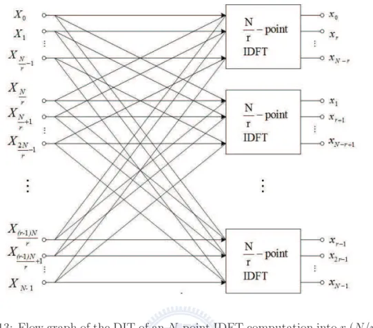
2.10 Flow graph of the DIF decomposition of an N-point IDFT computation into r × (N/r)-point IDFTs. . . . 16
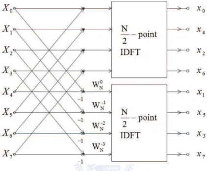
2.11 Flow graph of the DIT decomposition of an 8-point IDFT computation into two 4-point IDFTs. . . 18
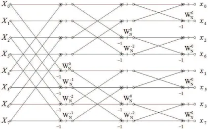
2.12 Flow graph of the complete DIT decomposition of an 8-point IDFT com-putation. . . 19
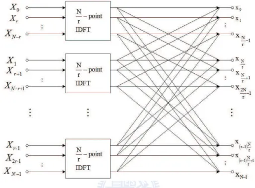
2.13 Flow graph of the DIT of an N-point IDFT computation into r (N/r)-point IDFT computations. . . 20
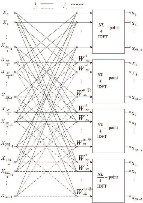
3.1 Flow graph of radix-4 DIT decomposition of an NL-point IDFT compu-tation into four (NL/4)-point IDFTs. . . . 24
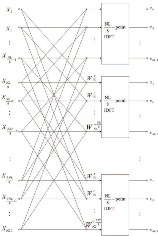
3.2 Flow graph of the radix-8 DIT of an NL-point IDFT computation into eight (NL/8)-point IDFTs. . . . 28
3.3 Flow graph of the radix-r DIT decomposition of an NL-point IDFT
com-putation into r × (NL/r)-point IDFT comcom-putations. . . . 31
3.4 Illustration of the proposed stop criterion (I). . . 32
3.5 Illustration of the proposed stop criterion (II). . . 33
3.6 Comparison of PAPR performance of Proposed SLM Scheme and conven-tional SLM Scheme. . . 38
3.7 Comparison of PAPR performance of Proposed PTS Scheme and conven-tional PTS Scheme. . . 39
3.8 Architecture of L&W Scheme I. . . 40
3.9 Architecture of modified convolution structure for generating candidate sequences. . . 41
3.10 Architecture of our proposed scheme with conversion vectors. . . 42
3.11 Comparison of PAPR reduction performance of the proposed modified
schemes I and II, LWW schemes I and II, and conventional SLM schemes. 46
3.12 Comparison of PAPR reduction performance of the proposed modified
scheme III, LWW scheme III, and conventional SLM scheme. . . 47
3.13 Comparison of PAPR reduction performance of the proposed modified schemes I and II, and the conventional PTS scheme. . . 48
3.14 Comparison of PAPR reduction performance of the proposed modified scheme III and the conventional PTS scheme. . . 49
4.1 Architecture of the proposed scheme. . . 52
4.3 Block diagram of the proposed new SLM scheme with vD = [1, 4] and
PD = [2, 8]. . . . 54
4.4 Comparison of the PAPR reduction performance of the proposed SLM
Scheme, G&G SLM scheme and conventional SLM scheme. . . 59
4.5 Magnitude of an equivalent phase sequence of our scheme. . . 60
4.6 Magnitude of an equivalent phase sequence of the G&G SLM scheme. . . 61
4.7 Comparison of the BER performance of the proposed SLM Scheme and the G&G SLM scheme. . . 62
List of Tables
3.1 The Proposed Algorithm . . . 34
3.2 Computational Complexity of Various Schemes (I) . . . 36
3.3 Computational Complexity of Various Schemes (II) . . . 36
3.4 Computational Complexity Ratio of the Proposed SLM Scheme with N = 256 . . . 36
3.5 Computational Complexity Ratio of the Proposed PTS Schemes with N = 256 and U = 8. . . . 37
3.6 Computational complexity of various SLM schemes (I) . . . 43
3.7 Computational complexity of various SLM schemes (II) . . . 43
3.8 Computational complexity of various PTS schemes (I) . . . 43
3.9 Computational complexity of various PTS schemes (II) . . . 44
3.10 Computational complexity ratio for Proposed SLM Schemes over the con-ventional SLM scheme with N = 256. . . . 44
3.11 Computational complexity ratio for Proposed PTS Schemes over the con-ventional PTS scheme with N = 256 and U = 8. . . . 45
4.1 Computational complexity of various SLM schemes (I) . . . 57
4.2 Computational complexity of various SLM schemes (II) . . . 57
4.3 Computational complexity ratio of the proposed SLM schemes with N = 256. . . 58
Chapter 1
Introduction
Orthogonal frequency division multiplexing (OFDM) has become a very popular transmission scheme for wideband communication systems due to its many desired prop-erties. For instance, it has high spectral/power efficiencies, admits simple channel esti-mation and equalization, is compatible with other anti-fading methods and allows flex-ible resource allocation. With all these advantages, it suffers from one major drawback: high peak-to-average power ratio (PAPR) of the resulting time-domain waveforms. The high PAPR effect often forces the transmit power amplifier backoff to avoid significant nonlinear signal distortion.
Various techniques have been proposed to deal with this issue [1]. These methods can be classified into three categories. The first category can be referred to as the block coding scheme [2]. A subset of legitimate signals with lower PAPR is transmitted instead of using the whole signal space, and a pre-defined mapping rule between information bit stream and signal subset has to be set up.
The second category includes several signal distortion schemes. Among them, clip-ping [3] is the simplest–it basically clips those parts of the signal whose magnitude exceed the predetermined threshold. Nevertheless, as clipping suffers from in-band distortion and out-band radiation, it results in spectral efficiency reduction and error rate perfor-mance degradation. Active constellation extension (ACE) [4] clips signal in time-domain and forces frequency-domain components to stay within an extended region so that no
BER degradation will occur. For tone reservation (TR) [5], the transmitter does not send data on s small subset of subcarriers, and find the specific time-domain signal to be added to the original time-domain signal to lower the value of PAPR. Tone injection (TI) [5] adjusts frequency-domain signal by choosing transmitted signal from alternative signal points to reduce peaks in time-domain.
The last category involves different signal scrambling schemes. In selective mapping (SLM) [6], an input frequency domain data block is multiplied by several predetermined sequences to generate the alternative sequences, and the one with the lowest time do-main PAPR is selected for transmission. In partial transmit sequences (PTS) [7], the input data block is partitioned into a number of disjoint subblocks, which are phase rotated by a set of phasors to produce a set of candidate sequences. The one with the lowest PAPR is chosen for transmission. Obviously, both SLM and PTS schemes need to perform multiple inverse fast Fourier transforms (IFFTs) and the associated com-putational complexity is often the main design concern that prevents their usages in a practical system.
In this thesis, we propose two new PAPR reduction approaches based on SLM and PTS schemes. In the first scheme, decimation-in-time radix-r IFFT algorithm is ex-ploited to transform an NL-point IDFT into two consecutive r × (NL/r)-point IDFT stages, with r being a adjusting parameter to produce different SLM and PTS alterna-tives. Unlike the conventional SLM and PTS schemes, phase sequences are applied to time-domain sequences and frequency-domain sequences respectively, phase sequences are multiplied to intermediate sequences between stage one and stage two. As a result, the calculation results of stage one are the same for all candidate sequences and just have to be calculated once for a given OFDM symbol. In addition, a stop criterion is also proposed to drop unnecessary calculations so that lower computational complexity is achieved and the same PAPR reduction performance as the conventional SLM or PTS schemes is provided.
It has been introduced in [12], the operations of IDFT can be replaced by conversion vectors. By performing circular convolution of IDFT of input data block and conversion vector with different number of right cyclic shift, a number of candidate sequences are generated. These conversion vectors are modified into our proposed scheme so that only
r × (NL/r)-point IDFTs are needed, and certain computational complexity is relieved
due to the reason mentioned in preceding paragraph.
The second proposed scheme generalizes the two-stage decomposition to a multiple-stage DIT radix-r IFFT implementation in which the values of r of multiple-stage one and the remaining stages can be different. For this multiple-stage SLM or PTS approach, phase sequences are multiplied to intermediate sequences within IFFT operations at more than one stage. Since the phase sequence generations are different from that of [16, 17], better PAPR reduction performance is achieved with the same computational complexity. Compares with the conventional SLM and PTS schemes, it achieves a lower computational complexity at the cost of slightly PAPR performance degradation. In other words, with the same complexity, our scheme provides better PAPR reduction performance than that of conventional schemes.
The rest of the thesis is organized as follow. The ensuing chapter provides a general description of OFDM systems and the associated PAPR problem. Detail description of the conventional SLM and PTS schemes is given in Chapter 2. In Chapter 3 we present our first DIT radix-r IFFT based scheme and a stop criterion for early termination. We also present schemes that combine our algorithm and the conversion vector approach of [12] in this chapter. In Chapter 4, we introduce a scheme which utilizes multiple-stage DIT radix-r IFFT to further lower the computational complexity. Analysis of compu-tational complexity and simulated PAPR curves of various approaches are provided in the related chapters. Finally, concluding remarks and suggestions for future studies are provided in Chapter 5.
Chapter 2
System Model and DFT/IDFT
Architectures
2.1
Orthogonal Frequency Division Multiplexing
Nowadays high data rate is desired in many applications. However, as the symbol duration decreases with increasing data rate, single carrier systems suffer from severer intersymbol interference (ISI) caused by the dispersive fading of wireless channels or equivalently, frequency selective fading channels. Therefore, a technique called orthog-onal frequency division multiplexing (OFDM) is introduced to cope with this problem.
The basic idea of OFDM is to divide the entire frequency selective fading channel into many narrowband flat fading subchannels. In other words, a high-rate data stream is split into several lower rate streams that are transmitted simultaneously over a number of subchannels, which can also be called subcarriers. Due to the increase of symbol duration for the lower rate streams, the relative amount of dispersion caused by the multi-path nature decreases. Furthermore, ISI can almost be completely eliminated with the aid of the cyclic prefix (CP) in which the OFDM symbol is cyclically extended to avoid intercarrier interference (ICI). The function of a CP is detailed later.
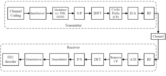
The block diagram of an OFDM system is provided in Fig. 2.1. The information bit stream is first encoded by a channel coding scheme (e.g. BCH code, convolutional code)
Figure 2.1: Block diagram of an OFDM system.
and then passed through an interleaver to increase the resistance to inferior frequency-selective channel conditions such as a deep fade. Serial-to-parallel (S/P) is used to generate the inputs of inverse discrete Fourier transform (IDFT) from the outputs of the modulator.
An OFDM symbol can be expressed as the sum of many independent signals modu-lated onto subcarriers. Let {Xk|k = 0, 1, · · · , N − 1} denote a block of N complex data
symbols modulated by phase shift keying (PSK) or quadrature amplitude modulation (QAM). The complex baseband representation of an OFDM symbol is given as
x(t) = 1 N
N −1X
k=0
Xkexp (j2πk∆f t) , 0 ≤ t ≤ T, (2.1)
where T is the OFDM symbol duration and ∆f = 1/T is the adjacent subcarrier sepa-ration. The discrete-time equivalent is the IDFT of {Xk} given by the following, with
time index t being replaced by sample number n,
xn= 1 N N −1X k=0 Xkexp µ j2πnk N ¶ , n = 0, 1, · · · , N − 1, (2.2) where {xn|n = 0, 1, · · · , N − 1} is the time-domain sequence. In practice, the IDFT can
be implemented efficiently by the inverse fast Fourier transform (IFFT) whose complex-ity can be reduced to O(N log2(N)) with the radix-2 algorithm.
In multipath channel, delayed replicas of the previous OFDM symbol lead to ISI between successive OFDM symbols. To eliminate the effects of ISI caused by the channel delay spread, a CP or guard interval is inserted between blocks of N IFFT coefficients, where the length of the CP is at least equal to that of the delay spread, such that multipath components from one symbol cannot interfere with the next symbol. The CP is simply a copy of the tail part of an OFDM symbol and can be attached to the front of the OFDM symbol. In this way, delayed replicas of the OFDM symbol always have an integer number of cycles within the FFT interval, as long as the delay spread is smaller than the length of CP or guard time. After appending the CP, the digital-to-analog converter (D/A) is involved to transform a discrete-time signal to an analog signal that passes to the radio frequency (RF) block. The RF block consists of up-converter, high power amplifier, and antenna. While the above-mentioned is the structure of an OFDM transmitter, the receiver is in a reverse operation with blocks having the inverse functions of those of the transmitter in the reverse order as depicted in Fig. 2.1.
2.2
Peak-to-Average Power Ratio
Since an OFDM symbol comprises a sum of modulated subcarriers, it is likely N sinusoids are added up coherently such that a large peak-to-average power ratio (PAPR) exists. When N signals are added with the same phase, N times peak power compare to average power is produced.
A large peak-to-average power ratio results in some disadvantages such as a reduced power efficiency of the power amplifier (PA). A large peak forces signal fall into the saturation region of the PA and causes nonlinear distortion. In such case, back-off is necessary for the power amplifier and its operating point is moved toward the origin to avoid signal from clipping. Hence, its power efficiency decreases proportionally with the back-off range. Even worse, nonlinear distortion may cause the degradation of bit-error rate (BER) performance. Therefore, a number of PAPR reduction schemes are proposed
to solve these problems.
While the discrete time PAPR of the transmit signal is defined as
P AP R = max 0≤n<N −1|xn| 2 E [|xn|2] , (2.3)
an L-oversampling is needed to ensure a negligible approximation error if the discrete PAPR analysis is to be used to approximate analog waveforms. The L-oversampling can be implemented by taking an NL-point IFFT on data block X concatenated with (L − 1)N zeros, that is, X = [X0, X1, · · · , XN −1, 0, · · · , 0]T. Therefore, the PAPR of the
transmit signal can be rewritten as
P AP R = max 0≤n<N L−1|xn| 2 E [|xn|2] . (2.4)
It is shown in [8, 9] that L = 4 can provide sufficiently accurate PAPR result. After knowing the drawbacks and the definition of PAPR, the measurement of it shall be introduced.
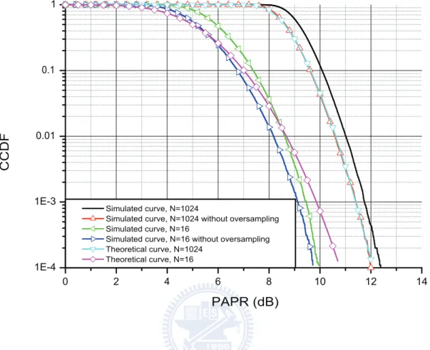
The complementary cumulative distribution function (CCDF) of the PAPR denotes the probability that the PAPR of a data block exceeds a given value is commonly used to measure the performance of PAPR reduction techniques. In [10], an approximate expression is derived for the CCDF of the PAPR for an OFDM symbol. From the central limit theorem we know that for a large value of N, the number of subcarriers
for the OFDM system, each time-domain signal sample xn is a circularly symmetric
complex Gaussian random variable with a mean of zero and a variance of 1. As a result, the amplitude of an OFDM symbol is Rayleigh distributed while the power distribution becomes a central chi-square distribution of two degrees of freedom with a cumulative distribution function (CDF) given by
CCDF of the PAPR per OFDM symbol, and this expression is given by
P (P AP R > z) = 1 − P (P AP R ≤ z)
= 1 − F (z)N
= 1 − (1 − exp(−z))N (2.6)
Equation shown above is obtained by assuming time-domain samples, xn, are mutually
independent. Theoretical curves and simulated curves are plotted in Fig. 2.2. We can notice that for the case of small N, (2.6) cannot approximate the true behavior well since the Gaussian assumption does not hold. Besides, this expression is not accurate anymore when oversampling is applied. Hence, in the following chapters, simulated curves are used to compare the performance of various PAPR reduction techniques, where the closer the CCDF curve is to the vertical axis, the better its PAPR characteristic.
2.3
Conventional Schemes for PAPR Reduction
To reduce PAPR of OFDM systems, it is possible to eliminate high peak values due to the constructive interference of time-domain signals with an identical phase by phase rotation. There are two methods, based on the rotation of phases of the subcarriers of a given OFDM symbol, that are commonly used; specifically , the selective mapping (SLM) and partial transmit sequences (PTS) schemes.
2.3.1
Selective Mapping
In the SLM technique, the input data block X = [X0, X1, · · · , XN −1]T is multiplied
element-wise by U phase sequences B(u) = [b(u) 0 , b
(u)
1 , · · · , b (u)
N −1]T, u = 1, 2, · · · , U , to
generate a set of alternative sequences which contain the same information as the original input data block where the first phase sequence B(1) is usually set to be an all-one
sequence. Thus, the uth alternative sequence is X(u) = [X
0b(u)0 , X1b1(u), · · · , XN −1b(u)N −1]T.
0 2 4 6 8 10 12 14 1E-4 1E-3 0.01 0.1 1 C C D F PAPR (dB) Simulated curve, N=1024
Simulated curve, N=1024 without oversampling Simulated curve, N=16
Simulated curve, N=16 without oversampling Theoretical curve, N=1024
Theoretical curve, N=16
Figure 2.2: Theoretical and simulated CCDF curves of the PAPR with N = 16 and
N = 1024. the candidates x(u)n = 1 N N −1X k=0 Xkb(k)k W−knN , (2.7)
where n = 0, 1, . . . , N − 1 and u = 1, 2, . . . , U , to choose from.
Among all the candidate sequences X(u), only the one with the lowest PAPR is
selected for transmission while the index u corresponding selected phase factor B(u) also
should be transmitted to the receiver as side information. For the implementation, the conventional SLM scheme needs U IDFT operations, and the number of required bits as side information is dlog2Ue for an input data block. This method is applicable to any
type of modulation and any number of subcarriers. A block diagram of the SLM scheme is depicted in Fig. 2.3.
Figure 2.3: Block diagram of the SLM scheme.
2.3.2
Partial Transmit Sequence
In an OFDM system employing PTS technique to reduce PAPR, an input data block is partitioned into M disjoint subblocks Xm = [Xm,0, Xm,1, . . . , Xm,N −1]T, m =
1, 2, · · · , M , where only specific subcarriers in the mth subblock Xm are nonzero and
the rest zero, i.e.,
M
X
m=1
Xm = X. (2.8)
Then, the subblocks Xm are trandformed into M time-domain partial transmit
se-quences, by NL-point IDFT operations, which are given as
xm= [xm,0, xm,1, · · · , xm,N L−1] = IDF T {Xm}. (2.9)
To reduce PAPR, these partial sequences are rotated by phase factors b = {bm =
ejθm|m = 0, 1, · · · , M − 1} independently. The PTS scheme is different from the SLM
scheme in that phase factors are multiplied by the time-domain signal and it can be demonstrated by the linearity property of the IDFT operation:
x0(b) = M X m=1 bm· IDF T {Xm} = M X m=1 bm· xm. (2.10)
In order to determine the optimum phase vector b0 which generates the candidate
sequence with the lowest PAPR, the following is employed: b0 = arg min b ½ max 0≤n<N L−1|x 0 n| ¾ . (2.11)
If W phase angles are allowed, e.g.,
θm ∈ ½ 2πi W | i = 0, 1, . . . , W − 1 ¾ , (2.12)
the number of all possible phase vectors is WM. The block diagram of the PTS scheme
is shown in Fig. 2.4. As we can see, in general, the conventional PTS scheme needs M IDFT operations for each input data block, and the number of required side information bits is dlog2WMe.
Figure 2.4: Block diagram of the PTS scheme.
Based on these two schemes, several new PAPR reduction schemes that are more efficient are proposed in the coming chapters.
2.4
Radix-r Algorithm
The IFFT algorithms are based on a divide-and-conquer approach which decomposes the computation of the IDFT of a N-length sequence into successively smaller IDFTs.
The fashion in which this principle is implemented results in a variety of different algo-rithms but all with comparable efficiency in computational speed. These algoalgo-rithms are most efficient when the number of data points N is highly composite and can be written as N = r1r2· · · rm, where r1, · · · , rm are all integers. Specifically, when N equals to rm,
where r is called the radix of the IFFT algorithm, a regular structure can be seen in the IFFT algorithm.
The divide-and-conquer approach can be achieved by either decimation-in-time (DIT) or decimation-in-frequency (DIF). To illustrate these two concepts clearly, N = 2m (i.e.
radix-2 algorithm)is considered in the following for the sake of simplicity.
2.4.1
Decimation-in-Frequency Algorithm
We first consider the DIF IFFT algorithm. It is mainly based on the decomposi-tion of the computadecomposi-tion into successively smaller IDFT operadecomposi-tions and thus results in substantial efficiency boost. The decomposition is done by breaking sequence Xk down
into successively smaller sequences. For N = 2m, an even integer, we can compute x n
by dividing the sequence Xk into two (N/2)-point sequences where one consists of the
even-numbered points and the odd-numbered points of Xk. With xn given by
xn= 1 N N −1X k=0 XkWN−nk, n = 0, 1, · · · , N − 1, (2.13)
where WN = e−j2π/N and dividing Xkinto its even-numbered and odd-numbered halves,
(2.13) becomes xn = 1 N Ã X k even XkW−nkN + X k odd XkW−nkN ! = 1 N (N/2)−1X s=0 X2sW−2snN + (N/2)−1X s=0 X2s+1W−(2s+1)nN = 1 N (N/2)−1X s=0 X2s(WN2)−sn + W−nN (N/2)−1X s=0 X2s+1(W2N)−sn (2.14)
where the second equality is due to the substitution of variables k = 2s for k even and
k = 2s + 1 for k odd.
It can be noted that each of the sums in (2.14) denotes an (N/2)-point IDFT with the first being the IDFT of the even-numbered points and the second that of the odd-numbered points of the original input data sequence. After the two IDFTs are computed, they are combined linearly according to (2.14) to generate the N-point IDFT xn. These
procedures can be illustrated by Fig. 2.5, where N = 8 is taken as an example, and can be repeated recursively until reaching 2-point IDFTs. A 2-point IDFT consists only of additions and subtractions of two points. and requires m = log2N stages of
computations. Figure 2.6 depicts the complete DIF decomposition of an 8-point IDFT
computation with m = 3 stages. We note that each stage has N complex
multiplica-Figure 2.5: Flow graph of the DIF decomposition of an 8-point IDFT computation into two 4-point IDFTs together with the proper linear combination.
tions and N complex additions. Since there are log2N stages, we have in total N log2N
complex multiplications and N log2N complex additions. Compared to the direct
com-putation of IDFT (2.13), which requires N2 complex multiplications and N(N − 1)
Figure 2.6: Flow graph of the complete DIF decomposition of an 8-point IDFT compu-tation.
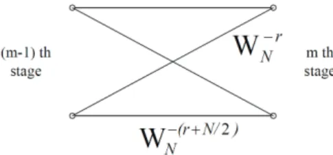
The amount of computation can be further reduced by exploiting the symmetry and periodicity of the complex coefficient W−n
N . We note that the basic computation to
obtain a pair of values in one stage from a pair of values in the preceding stage can be visualized by Fig. 2.7. From (2.14) and Fig. 2.6, it can be observed that the coefficients that linearly combine Xk’s are always powers of WN and exponents are separated by
N/2. Due to the symmetry property of WN, Fig. 2.7 can be transformed into Fig. 2.8.
Figure 2.7: Flow graph of the basic butterfly computation for Fig. 2.6.
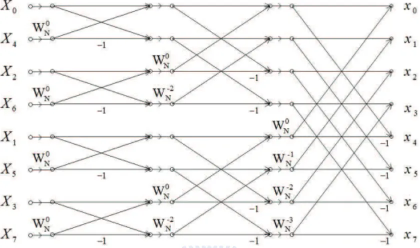
Accordingly, the computation of Fig. 2.7 can be simplified to Fig. 2.8, i.e. the required complex multiplication number is reduced from two to only one. Hence, by using the simplified form of the butterfly operation in Fig. 2.8, the total number of complex multiplications is (N/2) log2N and that of complex additions remains unchanged as N log2N. The simlified version of Fig. 2.6 is given in Fig. 2.9.
Figure 2.8: Flow graph of the simplified butterfly computation for Fig. 2.7.
Figure 2.9: Flow graph of the 8-point IDFT using the butterfly computation of Fig. 2.8.
As for general cases other than r = 2, DIF IFFT can be implemented by dividing the frequency domain components into r subsets
{Xrs}N L/r−1s=0 ;
{Xrs+1}N L/r−1s=0 ;
...
{Xrs+(r−1)}N L/r−1s=0 ,
and (2.14) can be generalized to
xn = 1 N (N/r)−1X s=0 Xrs(WrN)−sn+ W−nN (N/r)−1X s=0 Xrs+1(WrN)−sn+ · · · +WN−(r−1)n (N/r)−1X s=0 Xrs+(r−1)(WrN)−sn . (2.15)
The flow graph of (2.15) is demonstrated in Fig. 2.10, and those r × (N/r)-point IDFT can also be decomposed recursively in a similar manner as mentioned above into logrN
stages.
Figure 2.10: Flow graph of the DIF decomposition of an N-point IDFT computation into r × (N/r)-point IDFTs.
2.4.2
Decimation-in-Time Algorithm
On the other hand, the DIT algorithm is organized in exactly the opposite manner of that of the DIF algorithm. In other words, while the latter computes IDFT by forming
smaller subsequences of the input sequence Xk with some specific order, the IDFT
computation based on DIT divides the output sequence xn into successively smaller
subsequences and is introduced subsequently.
Similarly, without loss of generality, we consider the case when r = 2 for the con-venience of the explanation of the DIT algorithm. To construct DIT algorithms, let us consider computing separately the even-numbered time-domain samples and those odd-numbered. Again, starting form (2.13), we obtain the even-numbered time-domain
samples as x2s = 1 N N −1 X k=0 XkWN−k(2s), s = 0, 1, · · · , N/2 − 1, (2.16)
which obviously can be expressed as
x2s = 1 N (N/2)−1X k=0 XkW−k(2s)N + N −1 X k=N/2 XkW−k(2s)N . (2.17) = 1 N (N/2)−1X k=0 XkW−k(2s)N + (N/2)−1X k=0 Xk+N/2W−(k+N/2)2sN . (2.18)
Similarly, the odd-numbered time-domain samples are given by
x2s+1 = 1 N N −1 X k=0 XkWN−k(2s+1), s = 0, 1, · · · , N/2 − 1, (2.19)
and can be rearrange to
x2s+1 = 1 N (N/2)−1X k=0 XkW−k(2s+1)N + N −1X k=N/2 XkW−k(2s+1)N = 1 N (N/2)−1X k=0 XkW−k(2s+1)N + (N/2)−1X k=0 Xk+N/2W−(k+N/2)(2s+1)N . (2.20)
Because of the periodicity of W−2skN and W2
N = WN/2, W−(N/2)2sN = 1, and W −N/2
N = −1,
WN−2s(k+N/2)= W−2sk
N W−sNN = W−2skN , (2.21)
and (2.18) and (2.20) can be rewritten as
x2s = 1 N (N/2)−1X k=0 ¡ Xk+ Xk+N/2 ¢ W−sk N/2 (2.22) x2s+1 = 1 N (N/2)−1X k=0 ¡ Xk− Xk+N/2 ¢ W−kN W−ksN/2, (2.23)
where s = 0, 1, · · · , N/2 − 1. It can be noticed that both (2.22) and (2.23) are the (N/2)-point IDFT of two (N/2)-length sequences, which are respectively obtained by adding the first and the last half of the input sequence element-by-element for the former and subtracting the last half from the first half followed by the multiplication of W−k N
for the latter. Thus, the IDFT can be computed by forming two sequences based on the brackets in the summations of (2.22) and (2.23), then computing the (N/2)-point IDFTs of these two sequences to obtain the even-numbered and the odd-numbered time-domain samples. The procedure discussed in above is illustrated in Fig. 2.11 for the case of an 8-point IDFT.
Figure 2.11: Flow graph of the DIT decomposition of an 8-point IDFT computation into two 4-point IDFTs.
Analogous to what have beeb seen in the DIF decomposition, the process of (2.22) and (2.23) can be done recursively for the smaller size of IDFTs (i.e. (N/2)-point IDFTs). This is realized by combining the first and the last half of the input points, which are of length N/4 for each (N/2)-point IDFTs led in (2.22) and (2.23) and then computing (N/4)-point IDFTs. This process can be done until reaching 2-point IDFT. The number of arithmetic operations involved (N/2) log2N complex multiplications and N log2N
complex additions, thus making its computational complexity identical to that of the DIF one. For the 8-point example, the corresponding flow graph of the complete DIT decomposition is shown in Fig. 2.12.
Figure 2.12: Flow graph of the complete DIT decomposition of an 8-point IDFT com-putation.
For general r’s, we may consider the time-domain sequence xn in r batches as
{xrn}N/r−1n=0 ;
{xrn+1}N/r−1n=0 ;
...
{xrn+(r−1)}N/r−1n=0 ,
and the IDFT expression can be rewritten as
xrn+n0 = N r−1 X k=0 Ãr−1 X q=0 Xk+qN r W −(qNr )n0 N ! W−k(rn+n0) N (2.24)
where n = 0, 1, . . . , N/r − 1 and n0 = 0, 1, . . . , r − 1 is the index of the butterfly outputs.
The flow graph is summarized in Fig. 2.13.
To conclude this section, we examine the tendency of the two decomposition methods as the computation moves from a former stage to a latter one. Specifically, the DIT IFFT algorithm successively decomposes larger IDFTs into smaller IDFTs while the DIF-based one performs the opposite, i.e., it combines smaller IDFTs into larger IDFTs. Therefore, the DIF IFFT algorithm needs to perform all the IDFTs in each stage before deriving a single time-domain sample whereas it is not the case for the DIT-based one. Only one
Figure 2.13: Flow graph of the DIT of an N-point IDFT computation into r (N/r)-point IDFT computations.
of the IDFTs in each stage is required to obtain a single output. This nice property of the DIT-based IFFT enables an early discard of unsuitable candidates before obtaining its whole output samples.
Chapter 3
IDFT architecture aware PAPR
reduction schemes I
3.1
Proposed Algorithm
In the proposed algorithm, we take the radix-r DIT IFFT algorithm introduced in the previous subsection as the basic structure to develop a novel scheme that can reduce the computational complexity for PAPR reduction. Although N-point IDFT can be decomposed into log2N stages until reaching 2-point IDFT, here we exploit
two stages only and visualize the structure in Fig. 2.13. The most important step of our construction is the selection of the value of r for radix-r at the first stage, because different such values of can result in different corresponding schemes for PAPR reduction such as the SLM and PTS methods. Hence, we will introduce two categories of values of r which respectively lead to the corresponding SLM and PTS schemes with L-oversampling employed. By taking some properties of the L-oversampling into account, we suggest some efficient algorithms. The way how our proposal reduces the complexity will also be mentioned in the subsequent discussions.
3.1.1
Corresponding SLM Scheme
In the rest of this thesis, the operation of L-oversampling interpreted as the IDFT of an data block X padded with (L−1)N zeros, and the length of the IDFT input sequence becomes NL. Also note that as discussed previously, the oversampling of L = 4 folds is sufficient to provide accurate PAPR approximations in general and thus will be adopted throughout this work. Most importantly, efficient algorithms will be developed under this adoption.
As mentioned above, different values of r at the first stage result in distinct cor-responding schemes for PAPR reduction. Specifically, if r = L (L = 4) is chosen, the proposed algorithm can equivalently correspond to the SLM scheme, which rotates phases subcarrier-wise to lower the PAPR value of an input data block. As will be in-troduced later, when the radix-4 DIT-based IFFT is taken as the basic building block of our proposed algorithm, the corresponding SLM scheme can be obtained. Accordingly, an NL-point time-domain samples are partitioned into four subsets where each subset is the output samples of an (NL/4)-point IDFT. The mathematical expression of the output samples of the first (NL/4)-point IDFT is given as
x4s = 1 NL N L−1X k=0 XkW−(4s)kN L , s = 0, 1, · · · , NL/4 − 1, (3.1)
and can be expressed as
x4s = 1 NL N L 4 −1 X k=0 XkW−k(4s)N L + N L 2 −1 X k=N L 4 XkW−k(4s)N L + 3N L 4 −1 X k=N L2 XkWN L−k(4s)+ N −1X k=3N L4 XkWN L−k(4s) (3.2)
With substitutions of variables in the last three summation in (3.2), we obtain x4s = 1 NL N L 4 −1 X k=0 XkW−k(4s)N L + N L 4 −1 X k=0 Xk+N L 4 W −(k+N L4 )(4s) N L N L 4 −1 X k=0 Xk+N L 2 W −(k+N L 2 )(4s) N L + N L 4 −1 X k=0 Xk+3N L 4 W −(k+3N L 4 )(4s) N L = 1 NL N L 4 −1 X k=0 ³ Xk+ Xk+N L4 + Xk+N L2 + Xk+3N L4 ´ W−k(4s)N L . (3.3)
From (3.3), it can be noticed that the input samples of (NL/4)-point IDFT is linear combination among four components of L-oversampled input data sequence and there is an interval of NL/4 between adjacent components. Similarly, output samples of the rest three (NL/4)-point IDFTs are given as
x4s+1 = 1 NL N L 4 −1 X k=0 ³ Xk+ jXk+N L 4 − Xk+ N L 2 − jXk+ 3N L 4 ´ W−k N LW −k(4s) N L ; (3.4) x4s+2 = 1 NL N L 4 −1 X k=0 ³ Xk− Xk+N L 4 + Xk+ N L 2 − Xk+ 3N L 4 ´ WN L−2kW−k(4s)N L ; (3.5) x4s+3 = 1 NL N L 4 −1 X k=0 ³ Xk− jXk+N L4 − Xk+N L2 + jXk+3N L4 ´ W−3k N LW −k(4s) N L (3.6)
where, similar to (3.3), each input samples of them can be obtained by a linear com-bination among four interleaved components of the length-NL zero-padded input data sequence. The flow graph of (3.3) – (3.6) are illustrated in Fig. 3.1. The different part of these four subsets is the weighting for each components in summations and for each (NL/4)-point IDFT, the weighting W−kn0
N L multiplied on the input sample is required,
where n0 = 0, 1, 2, 3 denotes the index of (NL/4)-point IDFT.
Due to the fact that 3N zeros are padded at the end of the original sequence to achieve 4-oversampling, only the first element (Xk) in the brackets of (3.3) – (3.6) is
nonzero while the rest three elements (Xk+N L 4 , Xk+
N L
2 , and Xk+ 3N L
4 ) zero. Hence, for
these four (NL/4)-point IDFTs, the length-N L
Figure 3.1: Flow graph of radix-4 DIT decomposition of an NL-point IDFT computation into four (NL/4)-point IDFTs.
same as the original input data block X = [X0, X1, · · · , XN −1]T of length N when the
weighting W−kn0
N L is not considered. After the process of four (NL/4)-point IDFTs, the
length-NL time-domain samples can be obtained.
Now, the question is, how do we map this case in which radix-4 is considered at the first stage into the corresponding SLM scheme? The key is the position where the phase sequences are multiplied with the input data block X. In the proposed algorithm, phase rotation occurs at the input sequences of the four (NL/4)-point IDFTs. In other words, phase sequences which generate candidate sequences are multiplied by the original input sequence of the four (NL/4)-point IDFTs (3.3) – (3.6) or, equivalently, multiplied with the data block X and then with different W−kn0
NL for different (NL/4)-point IDFTs.
Therefore, the frequency-domain representation of the u-th candidate sequence can be expressed as
X(u) = XB(u) def= [X0b(u)0 , X1b(u)1 , · · · , XN −1b(u)N −1]T (3.7)
where u = 1, 2, · · · , U , U is the number of phase sequences, and B(u) = [b(u) 0 , b
(u)
1 , · · · , b (u)
N −1]T
is the uth phase sequence. Additionally, there are different weightings W−kn0 N L , n0 ∈
{0, 1, 2, 3} have to be multiplied prior or after X is multiplied by B(u) for different
(NL/4)-point IDFTs.
It can be noted from (3.7) that the subcarrier-wise multiplication of the phase factors and the input data block X makes our proposal identical to and be regarded as the conventional SLM scheme where r = L (L = 4). Furthermore, since phase sequences can be multiplied after the data X is scaled by weightings W−kn0
N L , we are able to improve the
conventional SLM scheme by the following: treating the calculation of the original inputs of the four (NL/4)-point IDFTs (3.3) – (3.6) as the first stage, and the multiplication of these input with B(u) the second. The computation result at the first stage of a specific
OFDM symbol can be calculated only once and stored and reused for U phase sequences at the second stage. Consequently, as opposed to the conventional SLM method, the proposed possesses lower computational complexity while preserves the same PAPR
reduction performance with the same number of subcarriers and phase sequences. As a final remark, we should mention that as long as NL/4 equals to a power of some r0, we can implement (NL/4)-point IDFTs efficiently by the radix-r0 IFFT where
r0 = 2 is most commonly used and will be adopted in our simulations.
3.1.2
Corresponding PTS Scheme
In this subsection, we propose an algorithm that corresponds to a complexity-reduced PTS implementation. Similarly, the required operations to derive the L-oversampled IDFT of input data block X is performed here. Again, as mentioned, the oversampling of 4-fold (i.e. 4-oversampling) is sufficient to accurately approximate the PAPR value of the time-domain signal that carries data X.
It has been mentioned in the beginning of this section that different values of r for radix-r at the first stage result in diverse corresponding schemes for PAPR reduction. In the following discussion, r > L (L = 4) is chosen to map this proposed algorithm to the corresponding PTS scheme, where r is a multiple of 4. For the conventional PTS scheme, the input data block is partitioned into M subblocks and phase rotation is operated block-wise, i.e., subcarriers belong to the same subblock are multiplied by the same phase factor to reduce the value of PAPR of the input data block X.
We first claim that the radix-r DIT IFFT algorithm with r > L and r being any multiple of 4 is the basic structure to correspond to a PTS scheme, without loss of generality, we may take r = 8 as an example to illustrate our proposal. According to the discussion in Section 2.4.2, NL-point time-domain samples are divided into eight subsets where each of them forms output samples of an (NL/8)-point IDFT. The mathematical expression of the radix-8 DIT IFFT algorithm is given by
x8s = 1 NL N L−1X k=0 XkW−k(8s)N L , s = 0, 1, · · · , NL/8 − 1, (3.8)
which is the expression of the first (NL/8)-point IDFT output and can be rewritten as x8s = 1 NL N L 8 −1 X k=0 ³ XkW−k(8s)N L + Xk+N L 8 W −(k+N L8 )(8s) N L + Xk+N L 4 W −(k+N L4 )(8s) N L + Xk+3N L 8 W −(k+3N L8 )(8s) N L + Xk+N L 2 W −(k+N L2 )(8s) N L + Xk+5N L 8 W −(k+5N L8 )(8s) N L + Xk+3N L 4 W −(k+3N L 4 )(8s) N L + Xk+7N L8 W −(k+7N L 8 )(8s) N L ´ = 1 NL N L 8 −1 X k=0 ³ Xk+ Xk+N L 8 + Xk+ N L 4 + Xk+ 3N L 8 + Xk+ N L 2 + Xk+ 5N L 8 +Xk+3N L 4 + Xk+7N L8 ´ W−ks N L 8 (3.9)
and, the rest (NL/8)-point IDFT output with n0 ∈ {1, 2, · · · , 7} are given collectively
as x8s+n0 = 1 NL N L 8 −1 X k=0 ÃÃ 7 X q=0 Xk+qN L 8 W −qn0 8 ! W−kn0 N L ! W−ksN L 8 , (3.10)
where q = 0, 1, · · · , 7 and s = 0, 1, · · · , NL/8 − 1. The flow graph of this radix-8-based algorithm is depicted in Fig. 3.2 with twiddle factors W−qn0
8 being neglected.
It can be observed from (3.9) and (3.10) that for a specific (NL/8)-point IDFT, each input sample is a linear combination among eight (NL/8)-equispaced components of the zero-padded input data sequence. Again, due to the padded zeros at the end of the original data, only the first two elements in the linear combinations of (3.9) and (3.10) are nonzero and the rest six zero. Hence, for each of these eight (NL/8)-point IDFTs, the actual input sequence is {Xk+ W−n8 0Xk+N L
8 |k = 0, 1, · · · , NL/8 − 1}, n0 ∈ {0, 1, · · · , 7},
which is of length N/2.
Similar to the case that corresponds to the SLM scheme, phase sequences which help generating candidate sequences are multiplied with the original input sequences that feed into these (NL/8)-point IDFTs. As will be detailed later, a same phase sequence have to be multiplied by the original input sequences element-wise for all (NL/8)-point IDFTs to generate a specific candidate sequence and to correspond to a PTS scheme.
Figure 3.2: Flow graph of the radix-8 DIT of an NL-point IDFT computation into eight (NL/8)-point IDFTs.
n0 = 0, 1, · · · , 7: x8s+n0 = N L 8 −1 X k=0 Ã 1 NL 7 X q=0 Xk+qN L 8 W −(k+qN L8 )(8s+n0) N L ! (3.11) the sum of the NL-point IDFTs of M = NL/8 subblocks
Xk = [0, · · · , 0| {z }, Xk, 0, · · · , 0| {z }, Xk+N L 8 , 0, · · · , 0, Xk+7N L8 , 0, · · · , 0| {z }] k NL 8 − 1 NL 8 − k (3.12)
where k = 0, 1, · · · , M − 1. Recall that the PTS scheme with M subblocks employed can be represented as (2.10). Therefore, it is possible to implement the corresponding PTS scheme via our proposal. Specifically, the implementation is given as
x08s+n0(B(u)) = M −1X k=0 b(u)k · IDF T {Xk} = 1 NL N L 8 −1 X k=0 ÃÃ 7 X q=0 Xk+qN L 8 W −qn0 8 ! W−kn0 N L ! b(u)k W−ks N L 8 (3.13)
where B(u) = [b(u) 0 , b
(u)
1 , · · · , b (u)
M −1]T, s = 0, 1, · · · , N L/8 − 1, and n0 = 0, 1, · · · , 7.
Ob-viously, just like the corresponding SLM scheme, the calculation in the outer brackets can be done beforehand and stored for the use by all phase sequences B(u), where
u = 1, 2, · · · , U and U is the number of candidate sequences. Since this calculation is
performed only once for a specific OFDM symbol, a great amount of computation is saved with PAPR reduction performance maintained.
For the general case of r > L (L = 4) where r is a multiple of 4, the mathematical expression of our radix-r decomposition is represented as
xrs+n0 = 1 NL N L r −1 X k=0 ÃÃr−1 X q=0 Xk+qN L r W −qn0 r ! W−kn0 N L ! W−ksN L r , (3.14)
where q = 0, 1, · · · , r − 1, s = 0, 1, · · · , NL/r − 1, n0 = 1, 2, · · · , r − 1. According to the
nonzero and the rest zero in the inner summations because of the zero-padding. There-fore, we have M = NL/r subblocks with each containing only r/L nonzero components. Analogous to the previous case, the corresponding PTS scheme can be implemented.
Again, finally, (NL/r)-point IDFTs are efficiently implemented by the radix-r0 IFFT
for r0 if NL/r is a power of r0.
3.1.3
Proposed Stop Criterion
A stop criterion is proposal in this subsection to further reduce the computational complexity by dropping unnecessary calculations. Before introducing this criterion, two points have to be highlighted.
First, recall the definition of the PAPR of a signal
P AP R = max 0≤n<N L−1|xn| 2 E [|xn|2] , (3.15)
where xn|n = 0, 1, · · · , NL − 1, are time-domain samples and L is the factor of
over-sampling. The set of allowed phase factors is written as P = {ej2πl/W |l=0,1,··· ,W −1 from
which elements of B(u) can choose, where W is the number of allowed phase factors
(angles). It can be noticed that all allowed phase factors locate on the unit circle, i.e. their magnitudes are all 1. We can show that for all U candidate sequences x(u) which
are the IDFT of X(u) derived via element-wise multiplication (3.7) or (3.13), their
ex-pected power Eh|x(u)n |2
i
is a constant if elements of B(u) are drawn from the polyphase
set P . Therefore, we can focus only on the peak value of each candidate sequence (the numerator of (3.15)) instead of calculating (3.15) wholely when choosing the one with the lowest PAPR in our proposed algorithms.
Second, as discussed in the previous subsections, the basic structure in our proposed algorithms is the radix-r DIT IFFT algorithm which owns a particular character that can be utilized to reduce the amount of calculations. Besides, from Fig. 3.3, it can be noted that the original NL-point IDFT is decomposed into r × (NL/r)-point IDFTs with linear combinations at the first stage and the output sequence of each (NL/r)-point
IDFT is a fraction of the length-NL oversampled time-domain samples. Therefore, the fact that in our proposed algorithms, these r × (NL/r)-point IDFT can be computed
sequentially enables us to early terminate the procedure for determining a candidate’s
PAPR immediately if its intermediate peak value already exceeds the minimum one calculated from the previous candidate sequences. In this way, needless calculations are avoided and thus the computational complexity decreased. In the following discussion, the detail of the proposed stop criterion is introduced.
Figure 3.3: Flow graph of the radix-r DIT decomposition of an NL-point IDFT com-putation into r × (NL/r)-point IDFT comcom-putations.
Our proposed stop criterion is executed by comparing and terminating. To launch this process, it is necessary to have a reference value for comparison. We take the corresponding SLM scheme with radix-4 at the first stage as an example and give some figures to illustrate the proposed stop criterion. Hence, in the beginning, the peak value of the candidate sequence without phase rotation X(1)= X, i.e. the original sequence, is
(NL/4)-point IDFT output of the ith candidate sequence for i = 2, 3, · · · , U and j = 1, 2, · · · , 4, is compared to.
We start from the second candidate sequence (i = 2), NL/4 time-domain samples are obtained after calculating the first (NL/4)-point IDFT. The peak value among these samples are found out and called P2,1 as shown in the frame of Fig. 3.4. Then,
Figure 3.4: Illustration of the proposed stop criterion (I).
P2,1 is compared to the reference peak value Pref. If P2,1 ≥ Pref, it can be figured
out from (3.15) that the PAPR value of the second candidate sequence, generated by the second phase sequence, must be larger than that of the time-domain samples of the original input data block. It is obvious that the second candidate sequence cannot achieve better performance of PAPR reduction, so the process to generate this candidate
sequence is terminated and the rest operations are dropped. Otherwise, the PAPR of this candidate sequence may be lower than that of the original input data, so the peak value of the second (NL/4)-point IDFT output samples P2,2 is necessary to be computed
and compared with Pref as depicted in Fig. 3.5.
Figure 3.5: Illustration of the proposed stop criterion (II).
As the same account mentioned above, comparing P2,2 with Pref is required to decide
whether this candidate sequence can achieve better PAPR reduction performance or not. If P2,2 ≥ Pref, we terminate the current process immediately, drop the rest processes to
generate this candidate sequence, and move on to the computation of the next candidate sequence. Otherwise, it is requested to calculate the peak value of the third (NL/4)-point IDFT output P2,3 and so on. Finally, if P2,4 is still smaller than Pref, it can be
Table 3.1: The Proposed Algorithm X(1) = [X 0, X1, · · · , XN −1] x = IDF T {X} Pref = max(|x|2) For u = 2 to U compute Pu,1; let s = 2;
while((Pu,j < Pref, j < s)&&(s ≤ r)) do
compute Pu,s;
s++; end
if((s − 1 = r)&&(Pu,r < Pref))
update Pref = max(Pu,j|j = 1, . . . , r);
end end
concluded that the PAPR of this candidate sequence is lower than that of the original input data block and Pref is updated by the largest among P2,j, j = 1, 2, 3, 4, and PAPR
of the second candidate sequence is recorded.
In general, based on the proposed stop criterion, r (NL/r)-point IDFTs are executed sequentially so that we can derive the peak value a part of the time-domain samples at a time. Therefore, the process of generating candidate sequence can be terminated once the peak value of a part of this candidate sequence already exceeds the reference
value Pref. The complete procedure is summarized in Table (3.1). As we can see
that unnecessary computations are neglected to lower the amount of computations. Accordingly, the computational complexity is reduced by employing the proposed stop criterion.
3.2
Performance Analysis and Comparison
3.2.1
Analysis of Computational Complexity
Compared to the conventional SLM and PTS schemes, our proposed radix-r DIT IFFT algorithm can reduce the computational complexity effectively on account of two reasons. First, each phase sequence is multiplied with the input of the r × (NL/r)-point IDFTs corresponding to the original data block X, so the computation result of the first stage for a given OFDM symbol can be preserved and used for all U phase sequences. In other words, the results of stage one for a specific OFDM symbol have to be calculated only once so that the computational complexity decreases. Second, by checking our pro-posed stop criterion sequentially, process of generating a particular candidate sequence can be terminated immediately once we are certain that this candidate sequence fails to reach a better PAPR reduction performance.
In order to compare the computational complexity of the proposed schemes and conventional schemes, we define the computational complexity ratio as
R = Complexity of proposed scheme
Complexity of conventional scheme × 100%.
The comparison of computational complexity is shown in Table 3.2 and 3.3, and the computational complexity ratio of various schemes is also given in Table 3.4 and 3.5. Note that the worst case complexity is adopted here to measure the performance of the proposal algorithms. As for the conventional PTS scheme, the number of subblocks (M) is replaced by NL/r, which is equivalent to the number of subblocks for our proposed PTS scheme, and r is the value of radix-r used at the first stage in our proposal.
3.2.2
Simulation Results
Simulations are performed to evaluate the PAPR reduction performance of the proposed corresponding SLM and PTS schemes. Here, the input data are 16-QAM
Table 3.2: Computational Complexity of Various Schemes (I) Number of complex multiplications Conventional SLM scheme U¡N L 2 · log2NL ¢ Proposed SLM scheme NL¡1 + U 2 · log2N ¢ Conventional PTS scheme (N L)2r 2 · log2NL
Proposed PTS scheme N L 2 ¡ log2r + U · log2 N L r ¢
Table 3.3: Computational Complexity of Various Schemes (II) Number of complex additions Conventional SLM scheme U (NL · log2NL)
Proposed SLM scheme NL (1 + U · log2N)
Conventional PTS scheme (N L)r 2 · log2NL
Proposed PTS scheme NL¡log2r + U · log2 N L r − 1
¢
modulated and the OFDM system contains N = 256 subcarriers. To estimate the PAPR, the OFDM symbol is oversampled by a factor of L = 4.
Figure 3.6 compares the PAPR performance of the proposed SLM scheme with pro-posed stop criterion and that of the conventional SLM scheme. It is seen that for a given number of candidate sequences (U), the PAPR reduction performance of the proposed, which is of lower computational complexity is identical to that of the conventional one. The PAPR reduction performance of the proposed and the conventional PTS scheme with number of candidate sequences set to be U = 8 is shown in Fig. 3.7. Again, noted that the proposed PTS scheme can achieve the same performance as the conventional one for a given number of subblocks (M) while having a lower complexity.
Table 3.4: Computational Complexity Ratio of the Proposed SLM Scheme with N = 256
Rmul (%) Radd (%)
U = 8 82.5 81.25
Table 3.5: Computational Complexity Ratio of the Proposed PTS Schemes with N = 256 and U = 8.
r = 32(M = 32) r = 128(M = 8) r = 256(M = 4)
Rmul (%) Radd (%) Rmul (%) Radd (%) Rmul (%) Radd (%)
U = 8 14.06 13.75 38.75 37.50 60 57.50
3.3
Proposed Algorithm with Conversion Vectors
In general, the SLM and PTS schemes can provide significant PAPR reduction per-formance, but each of them may require a high computational load due to the need of a bank of IDFTs. Therefore, we are interest in the methods which reduce the computa-tional complexity of both SLM and PTS schemes.
3.3.1
Brief introduction for LWW Scheme
It has been introduced in [12] that the IDFT operations were substituted for conver-sion vectors which are specified in the form of perfect sequences so that the corresponding phase sequences all have the same magnitude to avoid the degradation of BER perfor-mance. In [12], candidate sequences can generated by applying an NL-point circular convolution of the time-domain with conversion vector which are composite of base vec-tors. To reduce the computational complexity of the conversion process, the conversion vectors whose length are all NL have to comply with some constrains. Accordingly, three classes of conversion vectors were proposed in [12], and three novel low-complexity SLM schemes we called LWW Schemes were implemented with these three classes conversion vectors.
According to the discrete Fourier transform (DFT) properties, if a time-domain signal
xn is time-shifted by an amount of ∆ (resulting in a signal xn−∆), its frequency-domain
representation is simply multiplied by a phase shift term of −j2πk∆N . Besides, circular convolution in time-domain becomes multiplication in frequency-domain. Therefore, a candidate sequence can be generated by performing a circular convolution of the IDFT
4 5 6 7 8 9 10 11 12 13 1E-4 1E-3 0.01 0.1 1 U=32 U=8 C C D F PAPR (dB) Proposed SLM Scheme Original Conventional SLM Scheme
Figure 3.6: Comparison of PAPR performance of Proposed SLM Scheme and conven-tional SLM Scheme.
of input data block with these three classes conversion vectors, and various numbers of right cyclic shift of base vectors can obtained a number of candidate sequences. Figure 3.8 illustrates the architecture of LWW Scheme I where Ga1, Ga2, Gb1 and Gb2 are the
base vectors of conversion vectors Ga and Gb, respectively.
From Fig. 3.8, it can be noted that only one NL-point IDFT is required to generate a number of candidate sequences by performing circular convolution and cyclic shifts, the computational complexity can be reduced significantly for LWW Schemes at the cost of PAPR reduction performance.
4 5 6 7 8 9 10 11 12 13 1E-4 1E-3 0.01 0.1 1 M=32 M=8 M=4 CCDF PAPR (dB) Proposed PTS scheme Original OFDM Conventional PTS scheme
Figure 3.7: Comparison of PAPR performance of Proposed PTS Scheme and conven-tional PTS Scheme.
3.3.2
Modified LWW Scheme with Proposed Stop Criterion
To reduce the computational complexity of our proposal further, LWW Scheme is considered with some modifications. First, the NL-point IDFT is replaced by our pro-posed algorithm which has been introduced in previous section. The second modification is about the length of base vectors which is length-NL in LWW Scheme. To adapt the conversion vectors to our schemes, the length of base vectors have to be changed to NL/r. Figure 3.9 shows the architecture of convolution structure in which Ha1, Ha2, Hb1 and
Hb2 denote the base vectors after length modification (i.e. length-(NL/r)). Therefore,
the complete structure of our proposed scheme with conversion vectors is presented in Fig 3.10. Similarly, the computation of r × (NL/r)-point IDFTs are computed once for
Figure 3.8: Architecture of L&W Scheme I.
a given OFDM symbol, and a number of candidate sequences are generated by applying circular convolution of base vectors with the out samples of r × (NL/r)-point IDFTs.
Furthermore, since we can derive the length-(NL/r) output sequence which is a frac-tion of certain length-NL candidate sequence sequentially, the proposed stop criterion can also be considered in this modified scheme to lower the computational complexity.
3.3.3
Analysis of Computational Complexity
For all r × (NL/r)-point IDFTs, each of them only needs to be performed once for a given OFDM symbol when length-modified LWW Scheme is combined to our proposed algorithm. Therefore, our proposed schemes with length-modified conversion vectors result in lower computational complexity compares with conventional SLM scheme, con-ventional PTS scheme, and our proposed schemes in preceding section.
There are three LWW Schemes proposed in [12]. The scheme introduced in previous subsection is LWW Scheme I. LW Scheme II is constructed by combining LWW Scheme I and the conventional SLM scheme to enhance the PAPR reduction performance. Two